Gustavo Luiz C. M. de Abreu
gustavo@dem.feis.unesp.brSanderson M. da Conceição
enders83@yahoo.com.brVicente Lopes Jr.
vicente@dem.feis.unesp.brMichael John Brennan
mjbrennan0@btinternet.comUniv. Estadual Paulista – UNESP Department of Mechanical Engineering 15385-000 Ilha Solteira, SP, Brazil
Marco Túlio Santana Alves
mtsalves@hotmail.com Univ. Federal de Uberlândia – UFU Department of Mechanical Engineering 38400-902 Uberlândia, MG, BrazilSystem Identification and Active
Vibration Control of a Flexible
Structure
The aim of this paper is to illustrate the active control of vibration of a flexible structure using a model-based digital controller. The state-space model of the system is derived using a system identification technique known as the Observer/Kalman Filter Identification (OKID) method together with Eigensystem Realization Algorithm (ERA). Based on the measured response of the structure to a random input, an explicit state-space model of the equivalent linear system is determined. The model is used in a Linear Quadratic Regulator (LQR) to control the first two modes of vibration of a cantilever beam using a piezoelectric actuator/sensor pair. Experimental results demonstrate the efficacy of the proposed approach.
Keywords: Observer/Kalman Filter Identification (OKID), Eigensystem Realization Algorithm (ERA), optimal vibration control, piezoelectric smart structures
Introduction
Smart structures, which use actuators, sensors and a controller, can be used to suppress vibration in situations where passive measures are undesirable because of weight or space constraints. Frequently, piezoelectric actuators and sensors are used as they are light, cheap and convenient to bond to structures (Crawley and de Luis, 1987; Abreu et al., 2003). Lead zirconate titanate (PZT) is often used as an actuator because it is relatively stiff and couples well to a structure, and polyvinylidene fluoride (PVDF) is used as a sensor as it can be very thin and is light. In some cases the same element can be used as both an actuator and a sensor (Dosh et al., 1992).
Although actuators and sensors are crucial elements in the design of a smart structure, they are not the focus of this paper. The focus is on the design of the controller. Two generic types of controller can be used; one requires no model of the system and can be analogue (Gatti et al., 2007) or digital (Fuller et al., 1996), and the other requires a model of the structure to be controlled. The model based controller can be further subdivided into two types: one type uses a numerical model of the structure derived theoretically, using finite element models (Allik and Hughes, 1970; Tzou and Tseng, 1990), for example. The second type involves the determination of a model of the structure using measured input and output data (Wang et al., 1999). This paper concentrates on this approach, and demonstrates the procedure to design such a controller. The main objective is to investigate the combination of a system identification method and the optimal control technique to actively control vibration.
Ljung (1999) provides an excellent introduction to the subject of system identification, and describes the various methodologies that have been developed. Among the time domain methods, the Observer/Kalman Filter Identification (OKID) algorithm has shown to be efficient and robust (Juang et al., 1993; Juang and Phan, 2001), and has been applied to space structures, such as the Shuttle Remote Manipulator System (Scott et al., 1993). It has several advantages for the active vibration control application discussed here. First, it
assumes that the system is a discrete linear time-invariant (LTI) state-space system. Second, it requires only input and output data to formulate the model (no a priori knowledge of the plant is needed). Third, a pseudo-Kalman state estimator is produced, and lastly, any residual truncation errors will be small. Together with the OKID algorithm, the Eigensystem Realization Algorithm (ERA) (Juang and Phan, 2001; Juang and Pappa, 1985) generates a low order state-space model of the system to be controlled.
The design of an optimal controller for active vibration control has been studied by many researchers (Anderson and Moore, 1989; Lewis and Syrmos, 1995; del Rosario and Smith, 1997; Shen et al., 1999; Abreu et al., 2003). Here, a Linear Quadratic Regulator (LQR) is employed to design a control law for controlling the vibrations of a piezoelectric smart structure because it is a powerful technique for designing controllers even for complex systems.
The paper is organized as follows. Firstly, the OKID and ERA approaches are summarized, and the LQR control technique is employed to design the optimal control law. The next section describes the experimental work in which the model and the controller of an experimental beam, fitted with piezoelectric actuators and sensors is determined. Following this, real time control is implemented to demonstrate the efficacy of the approach. Finally, the paper is closed with conclusion section which contains some concluding remarks.
Nomenclature
= state matrix = input matrix = output matrix
= controller gain matrix = sampled time
= observer gain matrix = Hankel matrix dimension = Markov’s observer gain matrix = control vector dimension = state vector dimension
= solution matrix of the algebraic Riccati equation
, = controller design matrices = output vector dimension
= input vector
, = unitary matrices
= external load perturbation = state vector
= output vector = Markov parameters
Greek Symbols
Σ ΣΣ
Σ = diagonal matrix of positive singular values = scalar design parameter
Subscripts
e = relative to observer
Superscripts
T = relative to transpose ^ = relative to estimative
Identification of the Dynamic Model Using Vibration Excitation and Response Data
In this section an overview is given of system identification technique used to determine a model of the system to be controlled. It consists of two parts – the OKID method to determine the system’s Markov parameters, and the ERA to translate these into a state-space model of the system.
Description of the OKID technique
The OKID method was developed to compute the Markov parameters of a linear system, which are the same as the sampled impulse response of the system. It is a time domain method which can work with general response data such as random vibration, impulsive signals or chirps. First, the observer Markov parameters are calculated, then the system Markov parameters are determined recursively from the Markov parameters of the observer system. The process of system identification using this method is described in (Juang and Phan, 2001; Juang et al., 1993). In this section a brief overview of the process is given.
Consider first a general linear system expressed in discrete-time state-space form as
+ 1 = +
= + (1a,b)
where is an × 1 state vector, an × 1 input or control vector and a × 1 output vector. Matrices , , and are the state, input, output, and direct influence matrix, respectively. The integer k represents sampled time.
The input-output description of the system with zero initial conditions can be obtained from Eq. (1) recursively as
= ∑&'(%)* % − − 1 + (2)
where %= % and are the Markov parameters of the system – they are also samples of the system impulse response. For a lightly damped system, many Markov parameters are needed because the impulse response takes a long time to decay away. To reduce this number, an observer is introduced to artificially add damping and hence reduce the length of the impulse response of the combined system. If ( , ) is an observable pair, then there exists an observer of the form
, + 1 = - + − [ − - ]
= + - + + − (3a,b)
- = - +
The matrix can be interpreted as an observer gain matrix. Consider the special case where all eigenvalues of + are zero. Thus, the estimated state - converges to the true state after at most steps, where is the order of the system. Equation (3) then becomes
+ 1 = + + + − (4a,b)
= +
The input-output description of the system described by Eq. (4) is given by (for ≥ )
= ∑2'(1%
%)* [ − − 1 − − 1 ]3+ (5)
where
1%= 4 + % + − + % 5
= 41%( 1%6 5,
in which 1% and are the Markov parameters of the observer system. A particular feature of this type of observer is that the Markov parameters 1% will become identically zero after a finite number of time steps. A standard recursive least-squares technique is used to solve Eq. (5) and then the observer Markov parameters are computed. Once the Markov parameters of the observer system are identified, the actual system Markov parameters can be calculated. The relationship between the Markov parameters of the observer system and those of the actual system is given by
%= % = 1%( + ∑%'(&)*1&6 %'&'(+ 1%6 (6)
Once the system Markov parameters have been determined, a state-space model of the system can then be derived using the ERA, which is described in the following subsection.
Minimum realization of the system model using the ERA
The estimated state-space model (7, 7, 8, 7) of a system is determined from the system Markov parameters % obtained by OKID using the ERA. Details of this approach can be found in (Juang and Phan, 2001; Juang and Pappa, 1985), so only a brief overview is given here. The algorithm begins by forming the × block Hankel matrix , given by
, = 9
% %:( ⋯ %:<'( %:( %:6 ⋯ %:<
⋮ ⋮ ⋮
%:<'( %:< ⋯ %:6<'6
The order of the system is determined from the singular value decomposition of , 0 which is given by
, 0 = ΣΣΣΣ 3 (8)
where the matrices and are unitary matrices, ΣΣΣΣ is an × diagonal matrix of positive singular values, and is the order of the system. Defining a × matrix @A3 and an × matrix @B3 made up of identity and null matrices of the form
@A3= [A CA× <'( A]
@B3 = [B CB× <'( B], (9a,b)
a discrete-time minimal order realization of the system can be written as
7 =ΣΣΣΣ'(/6 3 , 1 ΣΣΣΣ'(/6 (10)
7 =ΣΣΣΣ(/6 3@B (11)
8 = @A3 ΣΣΣΣ(/6 (12)
and the direct influence matrix 7 can be identified by solving Eq. (5). Obviously, the 7, 7, 8, 7 matrices describe the state space model, which are functions of the singular values of the collected data. Note that now the state space variables allow one to give a clear physical meaning to the identified state-space system.
Optimal Controller Design
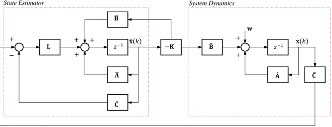
The state-space model given by Eqs. (10)-(12) obtained using the procedure given previously can be used to design an optimal controller. The control algorithm used here is an iterative version of the Linear Quadratic Regulator (LQR). The controller consists of a state feedback module and a state estimation module as shown in Fig. 1, in which the external load perturbation is , and is described in this section. The control law is given by
= − (13)
where is the matrix of feedback gains. These gains have to be determined while maintaining voltage levels less than a prescribed maximum level to prevent saturation of the actuators. Hence, a full state feedback control is considered to minimize the cost function given by (Anderson and Moore, 1989)
E =12 G[H 3 + 3 ]
&)(
(14)
where the matrix defines the relative weight of each state variable and stands for the relative weight of each actuator voltage.
Figure 1. Block diagram of the discrete-time LQR controller.
The selection of and is vital in the control design process. They determine the relative importance of the control performance and the control effort. A large puts higher demand on the control performance and a large puts a greater constraint on the control effort (Anderson and Moore, 1989). The optimal values for and are typically obtained by trial-and-error. The weighting matrix can be set as with as a scalar design parameter. Thus, the task of choosing and reduces to one of choosing . Consequently, the control performance, such as settling time and the maximum value of the actuator voltage can be tuned through changing the value of .
The optimal feedback gain matrix that minimizes the cost function in Eq. (14) is given by
= I + 73 7J'(73 7 (15)
where the positive definite matrix is the solution to the algebraic Riccati equation given by (Lewis and Syrmos, 1995)
73 7 − − 73 7I + 73 7J'(73 7 + = 0 (16)
In Eq. (13) it is assumed that all of the states are available for feedback. However, in practice only the system outputs are available for feedback. To estimate the states of the system from sensor outputs, a state estimator
- + 1 = 7- + 7 + 4 − 8- − 7 5, (17)
is required, in which - and denote the estimated state and the observer gain matrices, respectively. Note that the state vector in Eq. (13) should be replaced by the estimated state - .
K'( K'(
7
7
8
− 7
7 8
- −
+ + +
+
+
+
Since the system is observable, the dynamic observer gain is obtained by solving an algebraic Riccati equation corresponding to the assumed observer design matrices L (positive semi-definite) and L (positive definite). Thus, the observer poles should be selected so that it is much faster (by about a factor of 10) than the desired closed-loop poles of (7 − 7 ).
One of the merits of the LQR technique lies in the separation principle, which means that the design of the feedback and the estimator shown in Fig. 1 can be carried out separately.
Experimental Work
To demonstrate the system identification procedure and the subsequent controller design methodology an experiment was carried out. A single-input single-output system was chosen involving an aluminum cantilever beam as shown in Fig. 2. Although this appears to be a simple physical system, it was quite
challenging from the control point of view as the damping was very light. The aim of the experiment was to control the first two modes of vibration which occurred at 12.75 Hz and 78.85 Hz. To achieve this, a PZT actuator was bonded to one side of the beam, at the root, as shown in Fig. 2(a), and a PVDF sensor was bonded to the other side of the beam. The positions of actuator and sensor were chosen according to the methodology described in Abreu et al. (2003).
The dimensions of the aluminum beam were 350 mm × 42 mm
× 2 mm, the piezoceramic actuator patch (model QP10N) 50 mm × 20 mm × 0.254 mm (ACX, 2011), and the PVDF sensor 30 mm × 10 mm × 0.205 mm. The voltage amplifier and the charge amplifier shown in Fig. 2(b) were used to drive the actuator and to condition the signal from the sensor respectively. As only the first two modes of the beam were of interest, the cut-off frequency of the low-pass filter in the charge amplifier was set to 100 Hz.
(a) (b)
Figure 2. Photographs of the experimental setup: (a) the overall setup; (b) location of the piezoelectric sensor.
Identification of a Model for the Cantilever Beam
To identify a model of the system, the experimental setup shown in Fig. 3 was used. A dSPACE 1103 board together with the Matlab® and Simulink® software were used to generate and process the signals. The beam was driven with white noise through the PZT actuator and the beam response was measured using the PVDF sensor. A sampling frequency of 1 kHz was used.
The time histories of the applied voltage to the PZT actuator and the output voltage from the PVDF sensor are shown in Figs. 4(a) and 4(b), respectively.
Using the method described previously, the Markov parameters of the observer and the system were calculated, and consequently a state-space model of the cantilever beam was determined. As it was intended to control the first two modes of the system only, it was necessary to reduce the state space model. The Hankel norm model reduction technique (Gawronski, 1998) was used to generate a fifth order model of the system, the matrices of which are given by
7 = M N N N
O0.526 −0.010 −0.010 −0.037 0.0110 +0.996 +0.080 −0.002 0.003
0 −0.079 +0.996 −0.002 0.002
0 0 0 +0.879 0.475
0 0 0 −0.471 0.875XY
Y Y Z
(18)
7 = M N N N
O−0.001331−0.000371 +0.000139 −0.000143 +0.000653XY
Y Y
Z (19)
8 = [−1.7960 −0.0057 0.3621 0.1825 −0.5290] (20)
7 = −0.002572 (21)
The measured frequency response function (calculated from 15 averages) of the system (in terms of the voltage applied to the PZT actuator and the voltage measured from the PVDF patch) together with the reconstructed frequency response function from the model are shown in Fig. 5. It can be seen that the frequency response of the identified model is a reasonable match to the frequency response of the actual system for the first two modes.
Controller Design
As the controller was designed using an iterative procedure as discussed previously, some preliminary experiments were carried out with some initial control parameters set arbitrarily. The experiment was set up as shown in Fig. 3 but now the computer was set in control mode instead of system identification mode. The
Piezoelectric Actuator
(PZT) Charge Amplifier
(PVDF)
Piezoelectric Sensor (PVDF) Charge Amplifier
(Hammer)
Hammer Beam
controller was implemented using Matlab® and Simulink® software together with a PC and the dSPACE1103 board. Figure 6 shows a Simulink® block diagram of the controller.
The beam was excited at its free end by using the impact hammer (model PCB 086C04) shown in Fig. 2(a). The response of the beam was measured by the PVDF sensor, with and without control. The control gain matrix was then obtained by try-and-error for the maximum voltage applied to the piezo-actuator (150V). Using the following state weight matrices
= [×[ and = = 0.04, (22a,b)
the control gain matrix was calculated using Eq. (15) to give
= [−0.024 −3.203 0.916 −1.412 1.708] (23)
Figure 3. Experimental setup for model identification of the system.
(a) (b)
Figure 4. Time histories used in the system identification procedure (a) actuator and (b) sensor.
Figure 5. Experimental and numerical frequency response functions between the voltage applied to the PZT actuator and voltage from the PVDF sensor (a) magnitude and (b) phase.
As mentioned previously, the parameters and are determined by trial-and-error methods to most effectively control the structure. At the same time, these parameters are limited for the sake of the breakdown voltage of the piezoelectric actuator.
The next step was to design a dynamic observer for the stability of the closed-loop system. This could be obtained by treating
3, 3 as if they were , in the feedback control law design.
Using the weight matrices L= [×[ and L= 10'\, the optimal observer gain vector was found to be
= M N N N
O−18.0170.878 124.491 31.587 −116.898XY
Y Y Z
(24)
The controller and the optimal observer were then implemented and the results are presented in the following section.
Experimental Results
The time-domain results of the control experiment are given in Fig. 7. Figure 7(a) shows the open and closed-loop responses of the sensor voltage, and Fig. 7(b) shows the corresponding control voltage. 0 0.5 1 1.5 2 2.5 3 3.5 4 4.5 5
-150 -100 -50 0 50 100 150
Time (s)
A
c
tu
a
to
r
V
o
lt
a
g
e
(
V
)
0 0.5 1 1.5 2 2.5 3 3.5 4 4.5 5 -0.8
-0.6 -0.4 -0.2 0 0.2 0.4 0.6 0.8
Time (s)
S
e
n
s
o
r
V
o
lt
a
g
e
(
V
)
101 102
-80 -60 -40 -20
A
m
p
lit
u
d
e
(
d
B
)
101 102
-500 -400 -300 -200 -100 0 100
P
h
a
s
e
(
d
e
g
re
e
s
)
Frequency (Hz) Experimental Data
Numerical Model
Voltage Amplifier D/A Converter A/D Converter
Charge Amplifier Beam
PVDF
PZT
dSPACE
(a)
Initially the controller was turned off and the results of this test are shown in Fig. 7(a). It can be seen that the damping in the system was quite light as the vibration took a long time to decay away. Close examination of the time response showed that the beam was vibrating primarily in its fundamental mode, and the damping ratio for this mode was estimated to be about 0.06. The
experiment was then repeated, but this time with the controller turned on. From Fig. 7(a), it can be seen that the vibration decays away much more quickly demonstrating the effectiveness of the controller. The damping ratio in this case was found to be about
0.2. It is thus clear that the main effect of the control was to add more damping to the system.
Figure 6. Simulink® block diagram of the controller.
(a) (b)
Figure 7. Time histories from the control experiments in which an impulsive force was applied to the end of the beam using a hammer. (a) Voltage from the PVDF sensor, (b) control voltage applied to the PZT actuator.
Figure 8 shows the experimental open-loop and closed-loop frequency response functions determined from the time histories shown in Fig. 7(a) and the time history of the force applied to the beam using the instrumented hammer. It can be observed that the control system reduced the vibrations in the frequency range containing the first two modes, with the dominant effect being on the first mode of vibration, as discussed above. The vibration reduction level was smaller for the second mode due mostly to the actuator location. In Abreu et al. (2003), the problem of choosing the optimal location of the actuator for the maximization of the control energy applied in each mode of vibration is discussed.
Another relevant aspect that can be mentioned is that the LQR controller does not guarantee disturbance reduction at other locations along the beam. One of the studies undertaken to guarantee this important performance requirement was presented by Abreu and Ribeiro (2003), who developed a robust controller that minimizes the effect of disturbances over an entire beam.
Conclusions
This paper has described the system identification, controller design, and subsequent implementation to control the vibration of an aluminum beam, in which a PZT patch was used as a control actuator and a PVDF patch was used as the vibration sensor. The controller was designed by solving a standard optimal control problem, and required a state-space model of the system. This model was obtained using the OKID/ERA system identification technique, using input and output vibration data from the beam. Two modes of the beam were controlled. From the experimental results, it was observed that satisfactory performance of vibration attenuation was achieved. Although the system identification and control methodology was demonstrated on a simple one-dimensional structure in this paper, it can, in principle, be applied to more complicated structures with multi-input-multi-output control systems.
RTI Data
DAC
PZT
ADC
PVDF
K Ts z-1 Discrete-T ime
Integrator -K* u
B* u
L* u
D* u
C* u
A* u
10
0.1
0 0.2 0.4 0.6 0.8 1 1.2 1.4 1.6 1.8 2 -8
-6 -4 -2 0 2 4 6 8
Time (s)
S
e
n
s
o
r
V
o
lt
a
g
e
(
V
)
Control off Control on
0 0.2 0.4 0.6 0.8 1 1.2 1.4 1.6 1.8 2 -200
-150 -100 -50 0 50 100 150 200
Time (s)
C
o
n
tr
o
l
V
o
lt
a
g
e
(
V
(b)
Figure 8. Open- and closed-loop transfer functions of the beam in which an impulsive force was applied to the end of the structure using a hammer. (a) Magnitude, (b) phase.
Acknowledgements
The first author would like to thank FAPESP (Nº 2008/05129-3) for the financial support of the reported research. The authors acknowledge the financial support of CNPq Brazilian Research Agency and FAPEMIG through INCT-EIE.
References
Abreu, G.L.C.M., Ribeiro, J.F. and Steffen, V.J., 2003, “Experiments on Optimal Vibration Control of a Flexible Beam Containing Piezoelectric Sensors and Actuators”, Shock and Vibration, Vol. 10, pp. 283-300.
Abreu, G.L.C.M. and Ribeiro, J.F., 2003, “Spatial H∞ Control of a
Flexible Beam containing Piezoelectric Sensors and Actuators”, 17th
International Congress of Mechanical Engineering – COBEM 2003. ACX, 1996-2011, “Active Control eXperts”, Inc. All rights reserved, http://www.acx.com.
Allik, H. and Hughes, T.J.R., 1970, “Finite Method for Piezoelectric Vibration”, International Journal for Numerical Methods in Engineering, No. 2, pp. 151-157.
Anderson, B.D.O. and Moore, J.B., 1989, “Optimal Control: Linear Quadratic Methods”, Prentice Hall International, Inc.
Crawley, E.F. and de Luis, J., 1987, “Use of Piezoelectric Actuators as Elements of Intelligent Structures”, AIAA Journal, Vol. 10, No. 25, pp. 1373-1385.
Del Rosario, R.C.H. and Smith, R.C., 1997, “LQR Control of Shell Vibrations via Piezoceramic Actuators”, NASA Contractor Report 201673, No. 97-19.
Dosh, J.J., Inman, D.J. and Garcia, E., 1992, “A Self-sensing
Piezoelectric Actuator for Collocated Control”, Journal of Intelligent
Material, Systems and Structures, Vol. 3, No. 1, pp. 166-185.
Fuller, C.R., Elliott, S.J. and Nelson, P.A., 1996, “Active Control of Vibration”, Academic Press Ltd, San Diego, CA.
Gatti, G., Brennan, M.J. and Gardonio, P., 2007, “Active damping of a beam using a physically collocated accelerometer and piezoelectric patch actuator” Journal of Sound and Vibration, Vol. 303, Issues 3-5, pp. 798-813. Gawronski, W.K., 1998, “Advanced Structural Dynamics and Active Control of Structures”, Institute of Technology of P Institute of Technology of Pasadena, California, USA.
Juang, J.N. and Pappa, R.S., 1985, “An Eigensystem Realization Algorithm for Modal Parameter Identification and Model Reduction”,
Journal of Guidance, Control and Dynamics, Vol. 8, No. 5, pp. 620-627. Juang, J.N., Phan, M. and Horta, L.G., 1993, “Identification of Observer/Kalman Filter Markov Parameters: Theory and Experiments”,
Journal of Guidance, Control and Dynamics, Vol. 16, No. 2, pp. 320-329. Juang, J.N. and Phan, M., 2001, “Identification and Control of Mechanical Systems”, Cambridge University Press, New York.
Lewis, F. and Syrmos, V.L., 1995, “Optimal Control”, Wiley, New York. Ljung, L., 1999, “System Identification: Theory for the User”, Englewood Cliffs, 2nd Ed., NJ: Prentice-Hall.
Scott, M., Gilbert, M. and Demeo, M., 1993, “Active Vibration
Damping of the Space Shuttle Remote Manipulator System”, Journal of
Guidance, Control and Dynamics, Vol. 16, No. 2, pp. 275-280.
Shen, Y., Homaifar, A., Bikdash, M. and Da Chen, 1999, “Active Control of Flexible Structures Using Genetic Algorithms and LQG/LTR Approaches”, Proceedings of the American Control Conference, San Diego, California USA, pp. 4398-4402.
Tzou, H.S. and Tseng, C.I., 1990, “Distributed Piezoelectric Sensor/Actuator Design for Dynamic Measurement/Control of Distributed Parameter Systems: A Piezoelectric Finite Element Approach”, Journal of Sound and Vibration, Vol. 138, No. 1, pp. 17-34.
Wang, Z., Chen, S. and Han, W., 1999, “Integrated Structural and Control Optimization of Intelligent Structures”, Engineering Structures, Vol. 21, pp. 183-191.
100 101 102
-50 0 50
A
m
p
lit
u
d
e
(
d
B
)
100 101 102
-200 -100 0 100 200
P
h
a
s
e
(
d
e
g
re
e
s
)
Frequency (Hz) Control off
Control on