Ductile Damage Prediction in Sheet Metal Forming
and Experimental Validation
Dissertation presented to the Faculty of Engineering, University of Porto, as a requirement to obtain the Ph.D. degree in Mechanical Engineering, carried out under the supervision of Professor Abel Dias dos Santos, Assistant Professor, Faculty of Engineering, University of Porto, Professor José Manuel de Almeida César de Sá, Full Professor, Faculty of Engineering, University of Porto and Professor Francisco Manuel Andrade Pires, Associate Professor, Faculty of Engineering, University of Porto.
Pedro Manuel Cardoso Teixeira
Faculdade de Engenharia da Universidade do Porto
Porto
Investigação financiada pela Fundação para a Ciência e a Tecnologia (Ministério da Ciência, Tecnologia e Ensino Superior) através da Bolsa de Doutoramento SFRH/BD/31341/2006, no âmbito do POS_C - Desenvolver Competências - Medida 1.2 e do QREN - POPH - Tipologia 4.1 - Formação
À minha família
“(...) it is sometimes difficult to select the proper model for a given application. The simplest is often the more efficient event, even if it is not the most accurate.”
In: Jean Lemaitre Handbook of Materials Behaviour Models, Academic Press, 2001
v
AGRADECIMENTOS
Ao Professor Doutor Abel Dias dos Santos desejo exprimir a minha sincera gratidão pela oportunidade concedida de trabalhar nesta área científica, através desta dissertação. A sua orientação, apoio e disponibilidade, e por fim, o seu espírito crítico na revisão minuciosa do presente texto foram fundamentais para a coerência e concretização desta dissertação.Ao Professor Doutor José Manuel de Almeida César de Sá agradeço o incentivo e o seu esforço para proporcionar as melhores condições para a realização desta dissertação. Queria igualmente agradecer o apoio financeiro concedido para a participação em conferências, fundamental para a divulgação do trabalho realizado nesta dissertação.
Ao Professor Doutor Francisco Manuel Andrade Pires desejo agradecer a disponibilidade e auxílio prestado nas implementações numéricas. A sua revisão crítica do presente texto foi igualmente fundamental para a coerência do mesmo.
Ao INEGI - Instituto de Engenharia Mecânica e Gestão Industrial desejo agradecer, na pessoa do Presidente e Director do CETECOP - Unidade das Tecnologias de Conformação Plástica, Professor Doutor Augusto Duarte Campos Barata da Rocha, a disponibilidade de meios concedida durante a realização deste trabalho. As facilidades de acesso a diversas capacidades científicas e tecnológicas do INEGI tornaram possível a realização do trabalho experimental apresentado nesta dissertação.
A toda a minha família, os meus verdadeiros amigos, que sempre me apoiaram e incentivaram nas alturas mais difíceis, quero exprimir os meus profundos agradecimentos pela vossa compreensão e amizade ao longo desta caminhada. A vós dedico este trabalho.
À Fundação para a Ciência e Tecnologia, pelo apoio financeiro concedido através da Bolsa de Doutoramento SFRH/BD/31341/2006.
Finalmente, a todos os que directamente ou indirectamente contribuíram com o seu esforço e apoio na realização deste trabalho, o meu muito obrigado.
vii
RESUMO
Os processos tecnológicos de conformação plástica de chapa são hoje correntemente utilizados em diversas áreas de produção. A complexidade crescente dos produtos, a constante redução dos ciclos de desenvolvimento e as tendências actuais de utilização de materiais mais leves e mais resistentes colocaram novos desafios aos processos de conformação plástica de chapa. Para fazer face a estes desafios, existe uma crescente aproximação ao conceito de produção virtual, e em particular ao uso da simulação numérica por elementos finitos. Nas últimas décadas, tem sido dedicado um extenso esforço no desenvolvimento destas ferramentas numéricas e no estabelecimento de modelos matemáticos que permitam modelar o comportamento da chapa quando sujeita ao processo de conformação plástica. Um dos desafios principais está relacionado com a previsão da ocorrência de rotura, especialmente importante para a nova classe de materiais mais leves e mais resistentes. A presente dissertação pretende ser uma contribuição para a melhoria e desenvolvimento de modelos de previsão de rotura em processos de conformação plástica de chapas metálicas, no âmbito da teoria da Mecânica do Dano Contínuo. São introduzidas as definições escalar e de ordem superior para a variável de dano e são desenvolvidos os modelos constitutivos correspondentes, seguindo uma formulação termodinamicamente consistente. É dedicada uma atenção especial aos aspectos computacionais da implementação numérica dos modelos constitutivos desenvolvidos e aos temas relacionados com a sua integração num programa de elementos finitos comercial. Para avaliar o desempenho da estratégia proposta, foram realizados vários testes numéricos e os ensaios experimentais correspondentes de modo a determinar a precisão dos modelos propostos na previsão de rotura. Com o objectivo de determinar o evento mais restritivo no processo de conformação plástica de chapas metálicas, estricção ou rotura, é proposta uma abordagem conjunta entre um critério de instabilidade e um modelo de dano. O algoritmo para a integração numérica do modelo é descrito e a importância da abordagem é ilustrada por intermédio da comparação dos resultados numéricos com resultados experimentais obtidos por outros autores.Palavras-Chave: Dano dúctil; Conformação Plástica; Modelação Numérica; Rotura; Instabilidade plástica.
ix
ABSTRACT
Sheet metal forming processes are widely used in several production areas. The growing complexity of the products, the shortening of development cycles and the actual trends of using lighter and higher strength materials has placed new challenges to the sheet metal forming processes. To face these challenges, a successive approach to virtual production has arisen, namely to finite element numerical simulation. In last decades, an extensive effort has been dedicated in the development of these numerical tools and in the establishment of mathematical models that allow a better modelling of sheet metal behaviour under plastic deformation. One key challenge is related with failure prediction, especially important for the new class of lighter and more resistant materials. The present dissertation intends to provide a contribution in the improvement and development of reliable failure prediction models for the simulation of metal forming processes, within Continuum Damage Mechanics theory. Scalar and high-order definitions for the damage variable are introduced and the derivation of corresponding constitutive models is addressed, following a thermodynamically consistent framework. Particular attention is devoted to the computational issues of the numerical implementation of derived constitutive models and to aspects related to its integration into a commercial finite element code. To evaluate the performance of the proposed framework, several numerical tests and corresponding experimental testings were carried out in order to assess the robustness and accuracy of the proposed models in the failure prediction in sheet metal forming processes. With the aim of determining the most restrictive event in sheet metal forming, necking or fracture, an integrated approach between an instability criterion and a damage model is proposed. The algorithm for numerical integration of the model is addressed and the importance of the coupled approach is illustrated by means of a comparison with experimental results obtained by other authors.Keywords: Ductile damage; Sheet Metal Forming; Numerical modelling; Failure; Plastic instability.
xi
RÉSUMÉ
Les procédés de mise en forme de tôles minces sont largement utilisés dans plusieurs areas de la production. La complexité croissante des produits, la diminution des cycles de développement et les tendances actuelles de l'utilisation de matériaux plus légers et plus résistants ont engendré de nouveaux défis pour les procédés de mise en forme de tôles minces. Pour affronter ces défis, il ya un approchement à la notion de production virtuelle, et, particulièrement, à la utilisation de la simulation numérique par éléments finis. Dans les dernières décades, un grand effort a été consacré au développement de ces outils numériques et a l’établissement de modèles mathématiques qui permettent un meilleur modelage du comportement de la tôle sous déformation plastique. Un des principaux défis se rapporte à la prévision de la survenue de rupture, particulièrement important pour la nouvelle classe de matériaux plus légers et plus résistants. Cette dissertation aspire de offrir une contribution à l'amélioration et le développement de modèles de prévision de rupture en la simulation de procédés de mise en forme, en vertu de la théorie de la mécanique des l’endommagent continu. Les définitions scalaire et tensorielle pour la variable d'endommagement sont introduites et les modèles de comportement correspondants sont développés, à la suite d'une formulation thermodynamique cohérente. C’en porte une spéciale attention aux aspects de mise en œuvre du calcul numérique des modèles de comportement développés et aux questions liées à son intégration dans un programme commercial d'éléments finis. Pour évaluer la performance de la stratégie proposée, ont été effectuées plusieurs tests numériques et des essais expérimentaux correspondants pour déterminer l'exactitude des modèles proposés pour prédire la rupture. Afin de déterminer l’événement plus restrictif dans les procédés de mise en forme de tôles minces, striction ou rupture, on propose une approche commune entre un critère d'instabilité et un modèle d'endommagement. L'algorithme d'intégration numérique du modèle est décrit et l'importance de l'approche est illustrée par la comparaison des résultats numériques avec les résultats expérimentaux obtenus par d'autres auteurs.Mots-clés: Endommagement ductile; Mise en forme; Modélisation numérique; Rupture; Instabilité plastique.
xiii
CONTENTS
AGRADECIMENTOS v RESUMO vii ABSTRACT ix RÉSUMÉ xi CONTENTS xiii 1. INTRODUCTION 1 1.1 Motivation 11.2 Scope and layout of the thesis 6
2. TOPICS IN CONTINUUM MECHANICS AND THERMODYNAMICS 9 2.1 Kinematics of deformation and strain measures 9
2.2 Forces and stress measures 15
2.3 Fundamental laws of thermodynamics 19
2.3.1 Conservation of mass 19
2.3.2 Momentum balance 19
2.3.3 The first principle 20
2.3.4 The second principle 20
2.3.5 The Clausius–Duhem inequality 20
2.4 Constitutive theory 21
2.4.1 Constitutive axioms 21
2.4.2 Thermodynamics with internal variables 23 2.4.3 Phenomenological and micromechanical approaches 26
2.4.4 The purely mechanical theory 27
2.4.5 The constitutive initial value problem 27 2.5 Weak equilibrium. The principle of virtual work 28
xiv CONTENTS
3. FINITE ELEMENT METHOD 29
3.1 Definition of the initial boundary value problem 29 3.2 Spatial discretization of initial boundary value problem 30 3.3 Time integration and incremental solution procedures 32 3.3.1 Explicit dynamic finite element solution strategy 34 3.4 Local integration of constitutive equations 38
3.5 Contact with friction modelling 41
4. ISOTROPIC DAMAGE MECHANICS 45
4.1 Introduction 45
4.2 Physical aspects of internal damage in solids 46 4.3 Continuous Damage Mechanics developments 47
4.3.1 Original developments 47
4.3.2 Ductile damage 50
4.4 Lemaitre’s elasto-plastic isotropic damage theory 53
4.4.1 State potential and state relations 53
4.4.2 Dissipation potential and associated evolution equations 56
4.4.3 Damage threshold 59
4.4.4 Critical damage criterion 59
4.4.5 Computational aspects 60
4.5 Elasto-plastic isotropic damage model with anisotropic flow 60
4.5.1 Constitutive model 61
4.5.2 Integration algorithm 63
4.6 Simplified elasto-plastic isotropic damage model with crack closure 70
4.6.1 Crack closure effect definition 71
4.6.2 Tensile / compressive split of stress tensor 72 4.6.3 Crack closure effect on damage evolution 73
4.6.4 Simplified integration algorithm 74
4.7 Remarks on non-local formulations 79
5. ANISOTROPIC DAMAGE MECHANICS 81
5.1 Introduction. Higher-order nature of damage variables 81 5.2 Physical interpretation of a second order damage variable 83 5.3 Coupled elasto-plastic anisotropic damage theory 86
5.3.1 The constitutive model 87
5.3.2 Integration algorithm 95
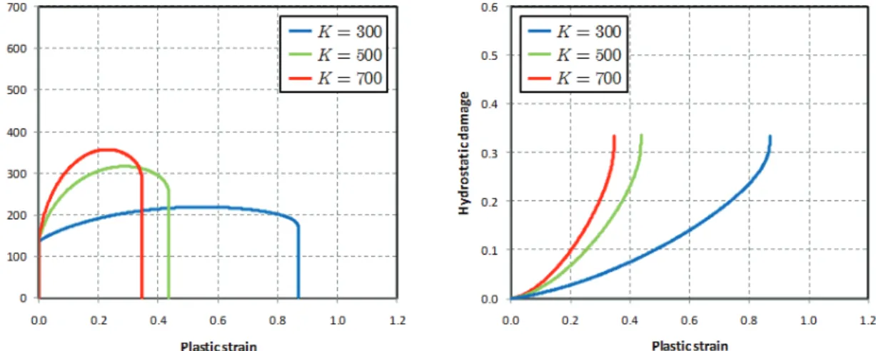
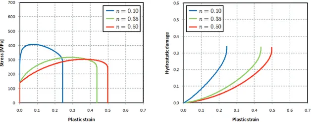
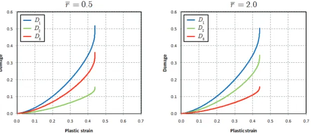
5.4 Sensitivity analysis of anisotropic damage model 102 5.4.1 Influence of damage evolution law parameters 102
5.4.2 Influence of hardening parameters 105
6. APPLICATION OF DAMAGE TO FAILURE PREDICTION 111
6.1 Tensile test 111
6.1.1 Numerical modelling 118
6.1.2 Results and discussion 119
6.2 Bulge test 122
6.2.1 Numerical modelling 124
6.2.2 Results and discussion 125
6.3 U shape geometry 130
6.3.1 Experimental failure 130
6.3.2 Numerical modelling 131
6.3.3 Results and discussion 131
6.4 Warping geometry 136
6.4.1 Experimental failure 136
6.4.2 Numerical modelling 137
6.4.3 Results and discussion 137
6.5 Axisymmetric cup 141
6.5.1 Experimental failure 142
6.5.2 Numerical modelling 142
6.5.3 Results and discussion 143
6.6 Cross shape geometry 152
6.6.1 Experimental failure 152
6.6.2 Numerical modelling 153
6.6.3 Results and discussion 154
6.7 Concluding remarks 160
7. APPLICATION OF DAMAGE TO NECKING OCCURENCE 163
7.1 Introduction 163
7.2 Forming limit diagrams modelling review 166
7.2.1 Hill’s localized necking criterion 167
7.2.2 Swift’s diffuse necking criterion (MFC) 169 7.2.3 Marciniak-Kuczynski analysis (M-K analysis) 172 7.2.4 Modified maximum force criterion (MMFC) 176 7.2.5 Other theoretical methods of necking prediction 180 7.3 Forming limit calculation with damage consideration review 181 7.4 Proposed damage-coupled criterion (MMFC+AD) 184 7.5 Application of MMFC+AD for forming limit diagrams prediction 187
7.6 Concluding remarks 199
8. CONCLUSION AND FINAL REMARKS 201
8.1 General conclusions 201
xvi CONTENTS
NOTATION, NOMENCLATURE AND ABBREVIATIONS 205
List of symbols 205 List of abbreviations 209 LIST OF FIGURES 211 LIST OF TABLES 215 LIST OF BOXES 217 REFERENCES 219
1
1. INTRODUCTION
This chapter establish the overall framework of the problems associated with the numerical simulation of metal forming processes, emphasizing on aspects such as the technological challenges and industrial interest. The objectives for the work developed in this thesis, based on the described challenges, are defined. The structure and contents of this dissertation, in order to guide the reader and to assist the consultation, are also presented.1.1 Motivation
Metal forming processes are characterized by the ability to obtain mechanical parts with high production rates with a minimum waste of material (near net-shape technology). Moreover, it is their high production rates that make these processes especially suitable for the production of components on a large scale. Among these technological processes, we may include those for making sheet metal parts. Terms like deep drawing, press working and press forming are used commonly in industry to describe general sheet forming operations, since they are performed usually on presses using a set of dies. Typically, a deep drawing operation implies the presence of three main components: a punch, a die and a blank holder. The principle of the process is illustrated in Figure 1.1.
The punch moves towards an initially flat metal sheet and deforms it in order to achieve a desired shape. The blank holder transfers an external force to the metal sheet, preventing wrinkling and allowing the control of the flow of the material. The two principal deformation modes in this process may depend directly on the blank holder action and its corresponding force. In the example presented in Figure 1.1, a tool used to draw an axisymmetric part is shown. However, deep drawing is also used to produce complex geometry parts, and, for some products and due to its inherent
2 Motivation Ch. 1
complexity, several deep drawing stages may be required to obtain a single final product, using several tool sets, one for each stamping stage.
Figure 1.1 Deep drawing process.
Sheet metal forming processes are used in several production areas and industries such as automotive, household appliances (washing machines, refrigerators, grills, stoves, etc.), domestic and decorative elements (bathtubs, dishwashers, containers, lamps, LPG cylinders, etc.), electrical and electronics (switches, computer and lamp socket components, etc.), food utensils (cookware, tableware, lids, trays, etc.), aerospace, ships, etc.
Current trends in these industries may be characterized by the flexibility and increasing complexity of products due to the demands imposed by the market. The strong competition among several producers coupled with increasing shortening of product life requires a rapid development of economic and high quality products, demanding a high flexibility for changes in design in order to fulfil the imposed innovation on such products [Yang 2002].
This reduction in development time cycle has left an extremely short period to the design of new tools and their correction and tuning. Typically, it takes many cycles and several costly trial-and-error stages in the development phase using prototype tools. The time consumption and press shop equipment occupation, needed for production, increase these development costs, compromising the necessary reduction in product-to-market cycle.
Among the industries that make use of sheet metal forming technology, we may emphasize the automotive industry due to its large production volumes and high variety of stamped components. The economic significance of this industry in developed countries associated with the strong competition among many producers creates vitality for the development of several knowledge areas including metal forming technologies.
Current main concerns in the automotive industry include environmental protection issues, fuel economy and safety specifications. The overall strategy incorporates the reduction of total vehicle weight, thus permitting to achieve better performances and fuel consumption reductions as well as decreasing greenhouse gas emissions. At the same time, the passenger’s safety must be continuously improved by addressing increasingly demanding safety specifications imposed by legislation. All these requirements have forced a policy of low weight concepts and structures prepared to withstand impacts [Pickett 2004], making use of lighter and / or more resistant materials.
However, the trend is not to have a single approach on the use of materials. The light, safe, clean and financially accessible car follows a multi-material concept, where different materials are used in body-in-white components of the vehicle, depending on the required strength for the part. The concept includes mild steels (MS), aluminium alloys (AA), conventional high strength steels (HSS) and advanced high strength steels (AHSS) such as dual phase steels (DP), transformation induced plasticity steels (TRIP) and martensitic steels (MS) [IISI 2006]. The introduction of new materials in the automobile industry has brought new challenges for metal forming technologies. The behaviour observed with conventional steels does not apply to these new materials and the empirical knowledge acquired over the years with conventional steels cannot be extrapolated to these new alloys, being needed the definition of new operating conditions.
These factors combined with the growing complexity of deep drawing technology led to a successive approximation to the virtual production concepts, in particular, the numerical simulation of metal forming processes by the finite element method and the extension of its use throughout all the production chain [Roll 2002].
The numerical simulation of metal forming has, therefore, assumed a vital role in satisfying the industry needs. The interest shown in these methods by the industry is evident: it allows to virtually validate a forming tool, reducing (or even replacing) the experimental tests on press, thus reducing the time-to market for new products and consequently the costs involved in its development. Still, the contribution of numerical simulation can go further, rather than being only confined to the simulation of the metal forming process and the validation of the manufacturability of the part. The optimization of the entire chain of production through the numerical simulation, starting from the raw material up to the final product, passing through assembling steps, aiming a cost reduction in each stage, can lead to significant gains in both economic and technical terms, crucial in the current highly competitive market. To achieve these higher objectives, several requirements are imposed to the numerical simulation [Makinouchi 2001]:
4 Motivation Ch. 1
• Simulation of all plastic forming process including stamping, cutting and folding;
• Reliability of numerical results in the prediction of forming defects including springback, wrinkling and fracture;
• Applicability to the wide variety of products produced by metal forming; • Use of different materials such as mild steels, aluminum alloys, high
strength steels and advanced high strength steels; • Obtaining results in reasonable time.
An extensive effort has been devoted over the last decades in the development of the numerical simulation codes focusing on the fulfilment of these requirements. Several areas are currently subject of intense research in order to approximate numerical simulation results to experimental reality: mechanical behaviour of materials and the establishment of constitutive laws to describe it, optimization of existing simulation codes, tribological aspects related to sheet / tool contact and the corresponding modelling, among others. The integration and interaction of information and developments collected in all these areas (extremely difficult) makes it possible the prediction of forming defects in the early stages of product development. The typical forming defects may range from small dimensional defects to extremely evident defects such as cracks and rupture. According to Lange [1985], forming defects can be classified into three distinct classes: dimensional defects, surface defects and defects related with unsatisfactory final mechanical properties. Other criteria such as aesthetic defects vs. functional defects or causes that originated them are also used to establish a distinction between different defects. A particularly broad criterion was proposed by Ajmar et al. [2001] that sets a differentiation between global and local defects. A defect is considered as a global defect if affects all the stamped part. A local defect is any defect that is limited to a restricted area of the part. This classification seems more appropriate to classify all forming defects, and can be applied to all types of defects, either aesthetic or functional, and can even be applied to defects for which the cause is unknown or is not perfectly defined. Following this classification, a list and classification of typical forming defects are presented in Table 1.1.
Traditionally, the major challenge was raised by the forming defects that were affecting the final geometry of the stamped part, namely the prediction of global defects related to springback [Santos 2008]. However, in the last years, fracture has assumed a prominent position. This trend is directly connected with the use of new materials, especially the Advanced High Strength Steels (AHSS), which present a
distinct mechanical behaviour, for which there is a smaller experience and prediction capability.
Table 1.1 Typical forming defects classification.
Forming defect Global Local
Twisting
•
3D Springback•
Wrinkles•
•
2D Springback•
Surface deflection•
•
Excessive thinning•
Rupture / cracks•
Marks•
Spoilers•
The application of these materials is intimately related with the obvious advantages that those materials can offer in terms of yield stress and tensile strength when compared to deep-drawing quality mild steels and conventional high-strength steels (HSS), as shown in Figure 1.2 [IISI 2006]. Their advantageous mechanical properties allow to produce lighter and more resistant components through the use of thinner sections, thus reducing the total structure weight and, in some cases, also allow the reduction of the number of components.
Figure 1.2 Different types of steels and their mechanical characteristics: Advanced high strength steels (AHSS) compared to mild steels (MS) and low-resistance and conventional high-strength steels (HSS).
But, these advantages in terms of weight, strength and stiffness of such components must be balanced with their lower ductility and premature rupture during processing. Fractures that rarely occurred a decade ago in resistance testings of the
6 Scope and layout of the thesis Ch. 1
components, have become frequent with the AHSS steels due to their lower ductility and its higher work hardening when compared with conventional steels. In these materials, failure often occurs before any necking occurrence and, therefore, without any notice, as seen in Figure 1.3.
Figure 1.3 Localized necking prior to the rupture in a DP600 steel (left) and fracture without any visible necking in a DP980 steel (right) [Shi 2006].
This behaviour raises questions to the applicability of conventional methods to assess forming limits, such as the well-established forming limit diagram (FLD) concept, which is defined for the occurrence of localized necking.
Therefore, the theoretical analysis of plastic instability and the initiation of fracture is of paramount importance for these materials in order to determine forming limits either by necking onset or by premature fracture occurrence. To model fracture initiation, a successive approximation is observed to theories that consider material inhomogeneities and describe the mechanism of internal damaging in ductile materials, either by using a micromechanics-based formulation [Gurson 1977] or a Continuous Damage Mechanics approach [Lemaitre 1985a]. The current trend for the failure prediction in forming simulations is to attempt the replacement of the common use of FLDs by a generalized incremental stress state dependent damage model, able to account for load-path dependent failure behaviour and to provide reliable prediction of the stress and strain histories, indispensable for predicting the onset of fracture in metals [Roll 2008].
1.2 Scope and layout of the thesis
The driven-force of this thesis is the ability enhancement of numerical codes for failure prediction in metal forming processes by the development of more advanced numerical models based on the Continuum Damage Mechanics theory. Therefore, the main objective of the present work is to contribute to the improvement and development of reliable failure prediction models for the simulation of sheet metal forming processes,
emphasizing issues related to continuum modelling as well as to the computational aspects relevant to the application of the proposed models in large scale numerical simulations in explicit time integration schemes.
In order to face this main goal, this thesis is divided into eight chapters. After this introductory one, Chapter 2 sets out the basic concepts of continuum mechanics and thermodynamics which form the basis for the constitutive model developments in the subsequent chapters. Also, with an introductory nature, the principles of finite element methods are introduced in Chapter 3.
Chapter 4 deals with the isotropic damage mechanics theory. A review of the basic concepts of internal damage in solids is provided and the developments under the Continuum Damage Mechanics theory are reviewed concerning different state and dissipation couplings. The original isotropic damage model proposed by Lemaitre [1985a] is presented and an enhancement of the model is introduced by the inclusion of plastic anisotropy described by the Hill48 criterion. A simplified partial coupling algorithm is proposed, which allows introducing additional effects without increasing dramatically the analysis time, namely the quasi-unilateral effect on damage evolution.
Chapter 5 introduces anisotropic damage mechanics. A review of higher order damage variables used to describe internal damage state of the material is presented and the physical interpretation of a second-order representation is provided. Using this latter definition, the thermodynamically consistent anisotropic damage model proposed by Lemaitre et al. [2000a] is described and its implementation into a commercial finite element code is addressed, also considering plastic anisotropic behaviour, as previously done for the isotropic damage theory. A sensitivity analysis of the implemented model is presented regarding the influence of several parameters on damage evolution and mechanical properties degradation.
Chapter 6 is mainly devoted to a qualitative validation of the implemented damage models and a discussion of the obtained results. Some basic classical testings and complex applications are considered in order to evaluate the performance of the models in the prediction of the ductile damage and failure that is expected to occur during metal forming processes. Intrinsically, a complete characterization of adopted damage models is achieved aiming to propose a methodology to virtually reproduce (or simulate) metal forming processes in order to predict when and where ductile failure will take place inside the stamped part.
Chapter 7 introduces a new criterion for forming limits prediction based on an integrated approach between the presented anisotropic damage model and the necking criterion proposed by Hora et al. [1996], combining the determination of the onset of the two last phases of plastic deformation: necking and failure. A review on forming limit diagrams modelling is provided and the most important criteria are presented.
8 Scope and layout of the thesis Ch. 1
The importance of the proposed coupled approach is shown by providing improved prediction in necking occurrence and allowing to determine which phenomenon, necking or failure, is the most restrictive event in a sheet metal forming operation, especially important in materials where fracture can occur before required conditions for necking are achieved.
Chapter 8 summarizes the main issues addressed in the thesis and cast the general conclusions of this work, along with suggestions for future research.
9
2. TOPICS IN CONTINUUM
MECHANICS AND
THERMODYNAMICS
This chapter reviews some basic concepts of mechanics and thermodynamics of continuous media. The objective is not to enter in full detail on the subjects, but to focus precisely on the points that have been employed and implemented throughout this work. The definitions and notation introduced will be systematically employed throughout the subsequent chapters of this thesis. The material presented here is well established in the continuum mechanics literature [Lemaitre 1994] [Simo 1998] [Doghri 2000] [Souza Neto 2008] and an effort has been made to follow the notation and nomenclature used in standard textbooks.2.1 Kinematics of deformation and strain measures
Consider a body B embedded in the three dimensional Euclidian space
R
3 in its reference (undeformed) configuration with boundary ∂B as represented in Figure 2.1 [Souza Neto 2008]. Each material particlep
can be labelled by its position in the orthogonal basis Ei. In its current (deformed) configuration, B occupies the region( )
ϕ B
defined by the deformation mapϕ
. The corresponding current position of particlep
can be defined as [Souza Neto 2008]:( )
=
x
ϕ
p
. (2.1)This description based on material coordinates is known as Lagrangian description. The corresponding vector field, which is the displacement, is defined by:
10 Kinematics of deformation and strain measures Ch. 2
( )
=
( )
−
u p
ϕ
p
p
(2.2)and, thus, one may write that:
( )
= +
x
p
u p
. (2.3)Due to the physical meaning of
x
andp
and by the fact that mapϕ
( )
⋅
is a one-to-one relation, deformation map can be uniquely inverted:( )
1 −=
p
ϕ
x
(2.4)where
ϕ
−1 is called reference map. This description, based on spatial coordinates, is known as Eulerian description.Figure 2.1 Configurations of a deformable body.
Now, consider an infinitesimal vector
dp
in the reference configuration. This infinitesimal vectordp
is transformed to its deformed statedx
, by the deformation gradientF
, as: d d d d = ⇔ = x x F p F p (2.5)or, alternatively, due to relation shown in Equation (2.3), deformation gradient can also be written as:
= + ∇
F I u (2.6)
where ∇u represents the gradient of displacement field.
Consider, now, an infinitesimal volume inside body B, defined by the infinitesimal vectors
d
a
,d
b
andd
c
. In the reference configuration, volume is expressed by:(
)
0
By applying the deformation gradient to the infinitesimal vectors, the deformed infinitesimal volume, denoted as
dV
, becomes:(
)
dV
=
F a F b F c
d
×
d
⋅
d
. (2.8) Making use of tensor algebra, it follows that:(
)
(
)
0 det d d d dV J dV d d d × ⋅ = = = × ⋅ F a F b F c F a b c (2.9)where
J
denotes the determinant ofF
, representing, locally, the volume after deformation per unit reference volume [Pires 2005]. In order to have a physically acceptable situation, in any deformation of a body,J
must be always greater than zero (otherwise infinitesimal volume would collapse into a point).The deformation gradient relates, therefore, quantities before deformation to quantities after deformation and provides a complete description of deformation including stretch as well as rigid body rotations. As rigid body rotations do not contribute for size and shape change of body B, it is imperative to decompose the deformation gradient
F
into stretch and rotation components [Pires 2005]. By applying the polar decomposition theorem, schematically represented in Figure 2.2, to the deformation gradientF
, one obtains:=
=
F
RU
VR
(2.10)where
U
is the right stretch tensor andV
is the left stretch tensor. The tensorR
is the local orthogonal rotation tensor and connects both configurations, reference and deformed configurations.12 Kinematics of deformation and strain measures Ch. 2
The two stretch tensors,
U
andV
, represent, in fact, measures of stretch itself since they only contain the stretch part of the deformation gradient. Therefore, polar decomposition is extremely important in the definition of strain measures, i.e., to define and quantify the change of distance between two particles between reference and deformed configurations. Before introducing strain measures, let us define the right and left Cauchy-Green stretch tensorsC
andb
, respectively given by:2 T
=
=
C
U
F F
,b
=
V
2=
FF
T. (2.11)Based on the right Cauchy-Green stretch tensor
C
, one can define an important family of strain measures, the Lagrangian strain tensorsE
. The most particular member of this family is the Green-Lagrange tensor, which is obtained as:( )2
1
(
2)
1
(
)
2
2
T
=
−
=
−
E
U
I
F F
I
. (2.12)Based on the left stretch tensor
b
, the Eulerian counterpart of the Lagrangian family tensors, denoted by ε, are defined as:( )
1
(
)
0
ln
0
m mm
m
m
⎧⎪⎪
−
≠
⎪⎪
= ⎨
⎪
⎡ ⎤
⎪
⎢ ⎥
=
⎪
⎣ ⎦
⎪⎩
V
I
V
ε
(2.13)where
m
is a real number andln ⎡ ⎤⋅⎢⎥⎣⎦
denotes the tensor logarithm of⎡ ⎤⋅⎢⎥⎣⎦
. Both Lagrangian and Eulerian strain tensors are related by:( )m ( )m T
= RE R
ε
(2.14)where
R
is a local rotation.So far, all these quantities were considered time-independent. However, many plasticity formulations are developed in terms of rate quantities [Dunne 2005], even the rate-independent plasticity models. Thus, it is important to consider a time-dependent deformation of body B, also called as motion. In this case, a deformation map
ϕ i
( )
,
t
defines the deformation of B for each timet
. Due to the time dependence of the motion, one can define velocity and acceleration of particlep
as being the first and second derivatives with respect to time as:( )
,
t
( )
,
t
t
∂
=
∂
p
x p
ϕ
;( )
( )
2 2 , ,t t t ∂ = ∂ p x p ϕ , (2.15)or, using an Eulerian description as:
( )
,
t
1( )
,
t
t
−∂
=
∂
x
v x
ϕ
;( )
( )
2 1 2 , ,t t t − ∂ = ∂ x a x ϕ (2.16)where
v
anda
are the spatial description of the velocity field and acceleration field, respectively.Considering a spatially varying velocity field
v
, it is also possible to calculate its spatial rate of change, given by the derivative of the velocity with respect to spatial coordinates as:x = ∇
l v (2.17)
where
l
is called the velocity gradient tensor. Considering the derivative of the deformation gradientF
with respect to time and applying the derivative chain rule, one may equivalently write that:1 −
=
l
FF
. (2.18)Therefore, velocity gradient maps the deformation gradient onto its rate of change. The velocity gradient tensor can be further decomposed into a symmetric tensor,
d
, called rate of deformation tensor or stretching tensor and a skew-symmetric tensor,w
, called continuum spin or vorticity tensor, defined as:( )
(
)
=
=
+
Td
sym
l
1
l
l
2
;=
( )
=
(
−
)
Tw
skew
l
1
l
l
2
. (2.19)Another definition is the skew-symmetric tensor
Ω
, also called angular velocity tensor. This tensor derives from tensorw
and defines only the rigid body rotation and its rate of change and is independent of the stretch. The angular velocity tensor is given by the expression:T
= RR
Ω
. (2.20)The importance of this tensor will be shown in the definition of stress rates. Further decomposition of the deformation gradient
F
can be performed, using the classical multiplicative decomposition theorem.Consider, again, a generic body B embedded in the three dimensional Euclidian space
R
3 in its reference (undeformed) configuration, containing an infinitesimal vectordp
, and the same body in its current (deformed) configuration, and the corresponding deformed infinitesimal vectordx
as seen in Figure 2.3 [Dunne 2005]. Additionally, consider an intermediate fictitious configuration of body B, corresponding to a stress-free state which infinitesimal vectordp
has undergone only purely plastic deformation to becomedX
. The transformation mapping ofdp
todX
is the plastic deformation gradient so that [Dunne 2005]:p
d
X
=
F p
d
(2.21)14 Kinematics of deformation and strain measures Ch. 2 p d d = X F p . (2.22)
Considering the current configuration
dX
, the transformation map ofdX
todx
is the elastic deformation tensorF
e given by:e
d
d
=
x
F
X
. (2.23)Figure 2.3 Schematic representation of the multiplicative decomposition theorem.
Thus, one may write:
e e p
d
x
=
F X
d
=
F F p
d
, (2.24) and, therefore: e p=
F
F F
(2.25)being this relation the classical multiplicative decomposition of the deformation gradient, into its elastic and plastic components. Using this decomposition, both the elastic and plastic deformation gradients may contain stretch and rigid body rotation resulting in a non-uniqueness intermediate configuration. By convention, and in order to achieve a unique intermediate configuration, rigid body rotations are affected to the plastic deformation gradient and as a result,
F
e andF
p can be written as:e
=
eF
V
;F
p=
V R
p (2.26)where
R
represents the total rigid body rotation between the initial and current configuration andV
e andV
p denote the elastic and plastic components of the left stretch tensor. Using this decomposition, one can redefine the velocity gradientl
andaddress the decomposition of the elastic and plastic rates of deformation. From Equation (2.18) and Equation (2.25) and after some straightforward tensor algebra, one may write the elastic and plastic components of the velocity gradient as a function of the elastic and plastic deformation gradients:
( )
1e
=
e e −l
V V
;l
p=
F F
p( )
p −1. (2.27)So, the velocity gradient can be rewritten as:
( )
1e e p e −
=
+
l
l
V l V
. (2.28) Performing the decomposition of this new definition of the velocity gradient into therate of deformation tensor
d
and the skew-symmetric continuum spin tensor,w
, (see Equation (2.19)), one has:( )
( )
( )
( )
1 1 1 1 sym sym skew skew e e p e e p e e e p e e p e − − − − ⎡ ⎤ ⎡ ⎤ = + ⎢ ⎥+ ⎢ ⎥ ⎢ ⎥ ⎢ ⎥ ⎣ ⎦ ⎣ ⎦ ⎡ ⎤ ⎡ ⎤ = + ⎢ ⎥ + ⎢ ⎥ ⎢ ⎥ ⎢ ⎥ ⎣ ⎦ ⎣ ⎦ d d V d V V w V w w V d V V w V . (2.29)Thus, it is possible to verify that elastic and plastic rates of deformation are not additively decomposed:
e p
≠ +
d d d . (2.30)
However, if elastic strains can be considered small, which is the case of metal forming processes, then the elastic part of the left stretch tensor
V
is almost equal toI
:( )
1e
=
e −≈
V
V
I
, (2.31)and it is possible to postulate the additive decomposition of the rate of deformation tensor as:
e p
= +
d d d . (2.32)
2.2 Forces and stress measures
In this section, the stress and equilibrium concepts for a large deformation analysis of a body will be introduced. The natural starting point for any description of stress measures is the Cauchy stress tensor. In order to introduce this definition, consider a body B in the deformed configuration, Figure 2.4 [Pires 2005]. Let
S
be an oriented surface of B with unit normal vectorn
at a pointx
.16 Forces and stress measures Ch. 2
Figure 2.4 Surface forces. The Cauchy stress.
Cauchy’s axiom states that: “At
x
, the surface force, i.e., the force per unit area, exerted acrossS
by the material on the side ofS
into whichn
is pointing upon the material on the other side ofS
depends onS
only through its normaln
.” This means that identical forces are transmitted across any surfaces with normaln
atx
. This force (per unit area) is called the Cauchy stress vector and will be denoted as [Souza Neto 2008]:( )
t n
(2.33)with dependence on
x
and time omitted for notational convenience. In the particular case when surfaceS
belongs to the boundary of B, the Cauchy stress vector represents the contact force exerted by the surrounding environment on B. Furthermore, the dependency of the surface forcet
on the normaln
is linear. This implies that there exists a tensor fieldσ
( )
x
such that the Cauchy stress vector is given by (Figure 2.4):( )
,
=
( )
t x n
σ
x n
. (2.34) The tensor fieldσ
is symmetric:T
=
σ
σ
(2.35)and is called the Cauchy stress tensor. It is often referred as the true stress tensor or, simply, stress tensor. Two important definitions (particularly convenient for the purpose of constitutive modelling) are obtained from the decomposition of the Cauchy stress tensor: the deviatoric stress or stress deviator and the spherical stress tensor. The deviatoric stress
s
is the traceless component of the stress tensorσ
and is given by:1 : 3 p ⎛⎜ ⎞⎟⎟ = − = −⎜⎜ ⊗ ⎟⎟ ⎜⎝ ⎠ s σ I I Ι Ι σ (2.36)
while the spherical stress tensor
p
I
, related with the first invariant of the stress tensor(
)
1
:
3
p
I
=
Ι
⊗
Ι σ
(2.37)where
p
is the hydrostatic pressure (also referred as hydrostatic stress) calculated as:( )
1
tr
3
p
=
σ
. (2.38)Other common definitions for stress tensors can be found in the literature. In practical nonlinear analysis, the most used alternative stress measures are the Kirchhoff stress tensor
τ
and the first and second Piola-Kirchhoff stress tensors,P
andS
, respectively given by:J
=
τ
σ
, (2.39) TJ
−=
P
σ
F
, (2.40) 1 TJ
− −=
S
F
σ
F
(2.41)where
J
is the volume ratio, as defined in Equation (2.9), andF
is the deformation gradient. From Equations (2.9) and (2.39), it is evident that, for incompressible deformation states (J
=
1
), there is no numerical distinction between the Cauchy and Kirchhoff stress tensors. Due to the symmetry of the Cauchy stress tensor, Kirchhoff stress is also a symmetric tensor. This is not usually the case of the first Piola-Kirchhoff stress tensor, Equation (2.40), which is generally unsymmetric. However, it is possible to devise a symmetric stress tensor by using the second Piola-Kirchhoff stress definition, Equation (2.41). In spite of the mathematical convenience, this tensor does not admit a physical interpretation in terms of surface tractions as the Cauchy stress.Despite these alternative stress tensors, Cauchy stress tensor is the most commonly used stress measure to establish equilibrium or constitutive equations. As for the strains, it is imperative to inquire the objectivity of tensor
σ
. The objectivity concept can be assessed by studying the effect of a rigid body motion superimposed on the deformed configuration (more details in Section 2.4.1.2) [Pires 2005]. A second order quantityG
is said to be objective if transforms as:T
→
G
QGQ
(2.42)being
Q
an orthogonal tensor describing an arbitrary superimposed rigid body rotation.To investigate material objectivity of Cauchy stress tensor, let us first apply a transformation to the normal and traction vectors by a rotation
Q
:( )
=( )
=t n Qt n
18 Forces and stress measures Ch. 2
Using the relationship between the traction vector and stress tensor,
t n
( )
=
σ
n
, in conjunction with the above quantities gives, one can write:( )
=
( )
⇔
( )
=
⇔
( )
=
Tt n
Qt n
t n
Q n
σ
t n
Q Q n
σ
, (2.44) and, so: T→ Q Q
σ
σ
. (2.45)Therefore, Cauchy stress tensor satisfies the objectivity requirement for a second order tensor, as defined in Equation (2.42), and is said to be objective.
The same material objectivity, however, is not ensured by the time derivative of the Cauchy stress tensor, which transformation reads:
T T T
→
Q Q
+
Q Q
+
Q Q
σ
σ
σ
σ
. (2.46)Only in the special case of a time-independent rotation, i.e., when
Q
=
0
, it is possible to say that Cauchy stress rateσ
is objective. Since plasticity problems are often formulated in a rate form, it is mandatory to define objective stress rates that ensure a transformation in accordance to Equation (2.42). These objective stress rates are usually defined by a suitable modification of the time derivative in order to satisfy material objectivity. The most common objective stress rates are the Jaumann-Zaremba, Truesdell and Green-Naghdi stress rates.The Jaumann-Zaremba stress rate, denoted as
σ
∇, is defined as: ∇ = −w + wσ σ σ σ (2.47)
where
w
is the continuum spin or vorticity tensor (Equation (2.19)). The Truesdell rate ofσ
, in the other hand, is defined as:( )
tr
T=
−
l
l
+
l
σ
○σ
σ − σ
σ
(2.48)where
l
is the velocity gradient tensor.The Green-Naghdi stress rate of tensor
σ
, here denotedσ
◊, is obtained by rotatingσ
back to the reference configuration, taking the time material derivative of the rotated quantity and then rotating the resulting derivative forward to the deformed configuration. That is:(
T)
T d dt ◊ = ⎡⎢ ⎤⎥ = − + ⎢ ⎥ ⎣ ⎦ R R R R σ σ σ Ωσ σΩ (2.49)2.3 Fundamental laws of thermodynamics
In order to model physical phenomena of deformation and failure, it is important to use a method based on the general principles that govern representative state variables of material continuum. In this section, some basic concepts in thermodynamics of continuum mechanics are introduced. For this purpose, let us define the scalar fields
θ
,e
,s
andr
defined over body B which represent, respectively, the temperature, specific internal energy, specific entropy and the density of heat production. In addition, variablesf
andq
denote vector fields of body force and heat flux, respectively.2.3.1 Conservation of mass
The first law of conservation postulates the conservation of mass expressed as [Pires 2005]:
divx 0
ρ+ρ u =
where
div
x⎡ ⎤⋅⎢⎥⎣⎦
denotes the spatial divergence. Expressing by words, this law states that mass of an isolated system cannot be changed as a result of processes acting inside the system.2.3.2 Momentum balance
The second law of conservation expresses the momentum balance. In its local form, balance can be expressed by the following partial differential equation with boundary condition [Souza Neto 2008]:
( )
( )
div
in
in
x+ =
ρ
=
∂
f
u
t
n
σ
ϕ
σ
ϕ
B
B
(2.50)where
n
is the outward unit vector normal to the deformed boundary of B andt
is the boundary traction vector field. The above momentum balance equations are formulated in the spatial (deformed) configuration. The corresponding formulation in the reference configuration is expressed in terms of the first Piola-Kirchhoff stress tensor as:div
in
in
pP
ρ
+
=
=
∂
P
f
u
t
m
B
B
(2.51)where
div
p⎡ ⎤⋅⎢⎥⎣⎦
denotes the material divergence,f
is the body force measured per unit reference volume,ρ
is the density in the reference configuration:J
20 Fundamental laws of thermodynamics Ch. 2
t is the boundary traction force per unit reference area and
m
is the outward normal to the boundary of B in its reference configuration.2.3.3 The first principle
The first principle of thermodynamics constitutes the third law of conservation related with the conservation of energy. It can be mathematically expressed by the equation [Pires 2005]:
: divx
e r
ρ =σ d+ρ − q (2.53)
where the product
σ
: d
stands for the stress power per unit volume in the deformed configuration. This principle states that the total energy inside an isolated system remains the same for any process occurring inside that system. Therefore, internal energy rate per unit deformed volume must be equal to the sum of stress power and heat production per unit deformed volume minus the spatial divergence of the heat flux.2.3.4 The second principle
The second principle of thermodynamics postulates that “energy systems have a tendency to increase their entropy rather than decrease it” and, therefore, expresses the irreversibility of entropy production. This principle can be expressed by the inequality:
divx r 0 s ρ ρ θ θ ⎡ ⎤ ⎢ ⎥ + ⎢ ⎥− ≥ ⎣ ⎦ q . (2.54)
2.3.5 The Clausius–Duhem inequality
The Clausius–Duhem inequality can be used to express the second law of thermodynamics for elastic-plastic materials and is a statement concerning the irreversibility of natural processes, especially when energy dissipation is involved. The Clausius–Duhem inequality derives from the fundamental inequality which, in turn, can be obtained by combining of the first and second principles of thermodynamics. Hence, the fundamental inequality is given by the expression:
(
)
1 divx : divx 0 s e ρ ρ θ θ ⎡ ⎤ ⎢ ⎥ + ⎢ ⎥− − + ≥ ⎣ ⎦ q d q σ . (2.55)Introducing a new variable, the specific free energy
ψ
(also known as Helmholtz free energy per unit mass) given by [Pires 2005]:e
s
ψ
= −
θ
(2.56)2 1 1 divx divx xθ θ θ θ ⎡ ⎤ ⎢ ⎥ = − ⋅ ∇ ⎢ ⎥ ⎣ ⎦ q q q (2.57)
into the fundamental inequality, one obtains the Clausius–Duhem inequality written as:
(
)
1
:
ρ ψ
s
θ
0
θ
−
+
−
⋅ ≥
d
q g
σ
(2.58)with g = ∇xθ. Assuming that intrinsic (mechanical) dissipation is decoupled from the thermal dissipation, both following equations must be satisfied simultaneously:
(
)
:
0
1
0
s
ρ ψ
θ
θ
−
+
≥
−
⋅ ≥
d
q g
σ
. (2.59)It should be noted that all presented principles are valid for all types of substances, either gases, fluids or solids as long as chemical and electromagnetic effects are not taken into account [Pires 2001].
2.4 Constitutive theory
The distinction between different types of material’s behaviour is made by introducing a proper constitutive model. Before starting to introduce the principles that are the basis for the constitutive theories presented in subsequently chapters, let us define the three fundamental axioms that define a rather general class of constitutive models of continua.
2.4.1 Constitutive axioms
The axioms, briefly presented in this section, must be satisfied for any constitutive model. It is important to make a distinction between thermokinetic and calorodynamic processes [Truesdell 1969]. A thermokinetic process of a generic body B is specified by a pair of thermokinetic variables:
( )
p
,t
ϕ
andθ p
( )
,t
. (2.60)For the body B at a given region of space
R
3 in which the thermokinetic process is occurring, the history of this process will be assumed to define a calorodynamic process or constitutive relations. The set of fields( ) ( ) ( ) ( ) ( ) ( )
{
σ
p
, ,
t e
p
, ,
t s
p
, ,
t r
p
, ,
t
f p
, ,
t
q p
,
t
}
(2.61) must satisfy the principles of thermodynamics and the momentum balance.22 Constitutive theory Ch. 2
2.4.1.1 Thermodynamic determinism
Thermodynamic determinism postulates that “the history of the thermokinetic process to which a neighbourhood of a point
p
of B has been subjected determines a calorodynamic process for B atp
”. For simple materials, the deformation gradientF
, the temperatureθ
and the spatial gradient of temperatureg
are sufficient to define the history of the thermokinetic process. Regarding all variables delivered by conservation laws and introducing the specific free energy, the principles of thermodynamic determinism implies the existence of constitutive functionalsF
,G
,H
andI
of histories ofF
,θ
andg
such that, for a pointp
, [Souza Neto 2008]:( )
(
)
( )
(
)
( )
(
)
( )
(
)
, ,
, ,
, ,
, ,
t t t t t t t t t t t tt
t
s t
t
θ
ψ
θ
θ
θ
=
=
=
=
F
g
F
g
F
g
q
F
g
σ
F
G
H
I
(2.62)and the Clausius–Duhem inequality holds for every thermokinetic process of B. 2.4.1.2 Material objectivity
Material objectivity axiom states that “material response is independent of the observer”. Assuming a change in the observer, a motion
ϕ
* is related with motionϕ
if it can be expressed as [Souza Neto 2008]:( )
( )
( ) ( )
* 0,
t
=
t
+
t
⎡
⎢
⎣
,
t
−
⎤
⎥
⎦
p
y
Q
p
x
ϕ
ϕ
(2.63)where
y
( )
t
is a point in space,Q
( )
t
is a rotation andϕ
( )
p
,t −
x
0 is the position vector ofϕ
( )
p
,
t
relative to an arbitrary origin x0. The deformation gradient corresponding to motionϕ
* is given by the transformation:*
=
F
QF
. (2.64)Scalar fields are unaffected by a change in observer but Cauchy stress
σ
, heat fluxq
and temperature gradientg
transform according to the rules:* * * T → = → = → = Q Q q q Qq g g Qg σ σ σ . (2.65)
This objectivity principle also imposes some restrictions to the functionals expressed in Equation (2.62), namely relations:

![Figure 1.3 Localized necking prior to the rupture in a DP600 steel (left) and fracture without any visible necking in a DP980 steel (right) [Shi 2006]](https://thumb-eu.123doks.com/thumbv2/123dok_br/15846054.1084959/22.892.167.735.243.470/figure-localized-necking-prior-rupture-fracture-visible-necking.webp)