The daily returns of the Portuguese stock index : a distributional characterization

WOR

CEEA

The D

Index

RKING P

AplA WP

Daily Re

x: A Dis

PAPER S

P No. 01/

eturns o

stributio

SERIES

/2013

of the P

onal Cha

S

Portugue

aracteri

ese Sto

ization

ock

dade dos Aç dade da Mad

çores deira

The Daily Returns of the Portuguese Stock Index: A

Distributional Characterization

Sameer Rege

CRP Henri Tudor

João C.A. Teixeira

Universidade dos Açores (DEG e CEEAplA)

António Gomes de Menezes

Universidade dos Açores (DEG e CEEAplA)

Working Paper n.º 01/2013

outubro de 2013

CEEAplA Working Paper n.º 01/2013 outubro de 2013

RESUMO/ABSTRACT

The Daily Returns of the Portuguese Stock Index: A Distributional Characterization

This paper compares the fitting of the normal, generalized hyperbolic, normal inverse Gaussian and Student t distributions to the daily returns of the Portuguese Stock Index PSI-20 over the period 1992-2013. We find that the distribution of the actual returns of the PSI-20 exhibits much higher kurtosis and extreme values as compared to the normal distribution. Overall, the best fit is provided by the Student t and the generalized hyperbolic distributions. This pattern also applies to the tail behavior, as the density of the Student t distribution exhibits fatter tails then the density of the other distributions, followed by the density of the generalized hyperbolic distribution. Finally, we find that the normal inverse Gaussian and the normal distributions have the lowest fitting quality to the actual daily returns of the Portuguese stock index. Keywords: normal distribution; generalized hyperbolic distribution; normal inverse Gaussian distribution; Student t distribution; Portuguese stock index returns. JEL classification: C5; G10 Sameer Rege CRP Henri Tudor 66 rue de Luxembourg L-4221 Esch-sur-Alzette Luxembourg

João C.A. Teixeira

Universidade dos Açores

Departamento de Economia e Gestão Rua da Mãe de Deus, 58

9501-801 Ponta Delgada António Gomes de Menezes Universidade dos Açores

Departamento de Economia e Gestão Rua da Mãe de Deus, 58

1

The Daily Returns of the Portuguese Stock Index:

a distributional characterization

Sameer R. Rege, João. C. A. Teixeira and António G. de Menezes1

This version: 28 October 2013

Abstract This paper compares the fitting of the normal, generalized hyperbolic, normal inverse Gaussian and Student t distributions to the daily returns of the Portuguese Stock Index PSI-20 over the period 1992-2013. We find that the distribution of the actual returns of the PSI-20 exhibits much higher kurtosis and extreme values as compared to the normal distribution. Overall, the best fit is provided by the Student t and the generalized hyperbolic distributions. This pattern also applies to the tail behavior, as the density of the Student t distribution exhibits fatter tails then the density of the other distributions, followed by the density of the generalized hyperbolic distribution. Finally, we find that the normal inverse Gaussian and the normal distributions have the lowest fitting quality to the actual daily returns of the Portuguese stock index.

Keywords: normal distribution; generalized hyperbolic distribution; normal inverse Gaussian distribution; Student t distribution; Portuguese stock index returns

JEL classification: C5; G10

1 _{Sameer R. Rege is at the Centre de Resources des Technologies pour l'Environnement, Luxembourg,}

and João C. A. Teixeira and António G. de Menezes and are at the Department of Economics and Business and at the Centre of Applied Economics Studies of the Atlantic, University of the Azores, Portugal. Corresponding author: João C. A. Teixeira (jteixeira@uac.pt). We would like to thank participants at the 2010 Portuguese Finance Network Conference in Ponta Delgada for helpful comments and discussions.

2

1 Introduction

Starting with the seminal work of Mandelbrot (1963) and Fama (1963), there has been a long standing interest in the financial literature for the identification of the return distribution of financial securities. The stock market crash of 1987 has highlighted the importance of the systematic study of the return distributions of financial instruments since from that moment it was clear that the real distribution of the percentage price change in stock market indices was not Gaussian. In fact, the financial literature seemed to agree that the probabilities of extreme values of log-returns in market indices, stocks and exchange rates were much larger than those predicted by the standard Gaussian distribution (Platen and Rendek, 2008).2

For the particular case of financial indices, it is now well documented that their return densities exhibit heavier tails and are more peaked than the Gaussian assumption (Fergusson and Platen, 2006). The most obvious stylized evidence that contradicts the normality assumption is the large excess kurtosis that is often observed. However, the literature has not been able to agree upon the best distribution that fits the returns of stock market indices. This paper contributes to this literature by comparing the fitting of the daily returns of the Portuguese Stock Index (PSI-20) provided by the generalized hyperbolic, normal inverse Gaussian, Student t and normal distributions.

The identification of the distribution that best fits the returns of stock market indices is of crucial importance since an invalid use of the normal distribution assumption can lead to series problems with the application of risk management instruments. For instance, by ignoring the skewness or kurtosis risk, many asset pricing models may simple misprice financial assets or derivatives. One obvious application where the incorrect measurement of skewness and kurtosis risk can lead to flawed

3

results in measuring the risk of a certain portfolio is the value-at-risk concept (VaR) since this concept still relies on the normality of the random variables.3

Our paper is closely related to the literature that has used the normal inverse Gaussian distribution, the generalized hyperbolic distribution and the Student t distribution in measuring the fitting of stock market returns. For the normal inverse Gaussian distribution our work relies on the paper by Barndorff-Nielsen (1995), while for the generalized hyperbolic distribution it relates to the studies by Barndorff-Nielsen (1978) and McNeil, Frey and Embrechts (2005). The study of the Student t distribution is also very relevant as Markowitz and Usmen (1996a, 1996b) analyzed the S&P500 log-returns in a Bayesian framework and they identified the Student t distribution as the best fit to daily log-return data of the S&P, whereas Hurst and Platen (1997) reached a similar result for the S&P500 and other regional indices.

The aim of this study is to compare the fitting performance of the normal inverse Gaussian, the generalized hyperbolic and the Student t distribution using daily data for the returns of the PSI-20. Most literature that addresses the distribution of stock market returns often uses quarterly data or yearly data. Also, it is well known that distributions of returns appear to come closer to normal distributions the longer the time horizon of measurement (Fergusson and Platen, 2006). Therefore, we believe that by using daily data we will be able to better identify fat tails on the data. We should also note that this is, as far as we are concerned, the first study to investigate the fitting of the normal inverse Gaussian, the generalized hyperbolic and the Student t distributions for a Portuguese stock index.

As far as the methodology is concerned, we use the Expectation-Maximization algorithm for maximum likelihood, as described by Karlis (2002), to estimate the

4

parameters of the normal inverse Gaussian distribution and the Student t distribution, and use the Nelder-Mead (1965) algorithm to estimate the parameter values of the generalized hyperbolic distribution.

The results show that the actual returns are characterized by much higher kurtosis and extreme values as compared to the normal distribution. Also, a global comparison of the histogram of the daily returns with the densities of the distributions reveals that the generalized hyperbolic distribution closely follows the histogram of actual daily returns, whereas the normal inverse Gaussian has a fit close to the normal distribution. A detailed analysis of the behavior of the distributions at the tails shows that the Student t distribution provides the best fit to the atual returns, followed by the generalized hyperbolic distributions. With lower fitting quality we find the normal inverse Gaussian and the normal distributions.

This paper is organized as follows. First, in Section 2, we introduce the framework characterizing the generalized hyperbolic, the normal inverse gaussian and the Student t distributions. Then, in Section 3, we discuss the procedure used to estimate the parameters of the distributions by describing the maximum likelihood test for this class of distributions. In Section 4 the application of this methodology to the stock market data provides the statistical tests and the corresponding estimated parameters and significance levels, allowing us to discuss the fitting of the distributions. Section 5 concludes.

5

2 The Index Returns Distributions

In this section we characterize the generalized hyperbolic, the normal inverse Gaussian and the Student t distributions by presenting the expressions for their density functions, moments, mean and standard deviations.

2.1 Generalized Hyperbolic distribution

The generalized hyperbolic (GH) distribution, introduced by Barndorff-Nielsen (1977), is a continuous probability distribution that belongs to the family of normal variance mixture distributions. The random variable is said to have a normal mean-variance mixture distribution if

√ (1)

where ~ 0,1 is standard Gaussian. Here 0 is a nonnegative random variable which is independent of , is a parameter for location and is a parameter for skewness.

The dimensional density function of the generalized hyperbolic distribution has five parameters: the location parameter and the skewness previously mentioned, for scale and and for change in tails.4 _{The distribution of ~ , , , , ,}

for , is characterized by its density:

, , , ⁄ ⁄ (2)

where , , , is given by:

, , ,

⁄

√ ⁄ (3)

6

and is a modified Bessel function of the third kind with index , as introduced by Abramowitz and Stegun (1972), 0 and 0 | | .

Moreover, this density function can be obtained by assuming a generalized

inverse Gaussian (GIG) distribution for the mixing density with ~ , , , where

e (4)

and .

Note also the resulting convenient representation for 1 2⁄ , with 0,1,2 …, where the Bessel function is expressed as:

⁄ ⁄ 1 ∑ _{! !} ! (5)

and , implying that ⁄ ⁄ ⁄ .

In order to obtain the various moments of the distribution, we first define its characteristic function. Denoting it by , Barndorff-Nielsen (1977) show that this is given by:

⁄

6

Furthermore, if the define as the natural logarithm of the characteristic function, i.e. , the various moments of the distribution are as follows:

7

8

7

10

where √ 1 is the imaginary number and , , , and denotes the first, second, third and fourth derivatives, respectively, of with respect to t, evaluated at 0.

It then follows that the mean, , and the variance, , of the generalized hyperbolic distribution are given by:

11

12

with .

2.2 Normal Inverse Gaussian distribution

There are several special cases of the generalized inverse Gaussian distribution but we will focus in particular in the normal inverse Gaussian (NIG) and the Student t distributions as these are widely used in finance since Barndorff-Nielsen (1995) and Praetz (1972) proposed log-returns to follow these mixture distributions, respectively. As far as the normal inverse Gaussian distribution is concerned, the corresponding density arises from the generalized inverse Gaussian density when the shape parameter

1 2⁄ is chosen. For this parameter value the variance is inverse Gaussian distributed and it follows from (2) that the density function is

8

where and , 0 and 0 | | . The mixing distribution of the NIG is the Inverse Gaussian (IG), and therefore we have that ~ , where

√ e z e 14

It also follows that the characteristic function of the NIG distribution is defined as:

15

and the mean, , and the variance, , are given by:

16

⁄ 17

2.3 Student t distribution

The Student t distribution has been identified by Praetz (1972), Blattberg and Gonedes (1974), Fergusson and Platen (2006) and Platen and Rendek (2008) to model the log-returns of financial securities. It is another special case of the generalized hyperbolic distribution with 2 degrees of freedom and shape parameters 0 and 0, that is 0 and √ . The Student t density function for the log-return is therefore defined as:

√ 1

µ

18

for , where Γ . is the gamma function. The log-return has mean µ, variance

9

the tail heaviness of the density, which implies a larger probability of extreme values. Moreover, as the degrees of freedom increase such that ∞, the Student t density approaches asymptotically the normal density.

3 Estimation of Distribution Parameters

Having identified the theoretical framework of the two distributions, we now discuss the procedure used to estimate the parameters of the distributions.

3.1 Normal Inverse Gaussian distribution

In order to estimate the parameters of the NIG distribution we use the Expectation-Maximization (EM) algorithm for maximum likelihood, as described by Karlis (2002). Karlis (2002) highlights that the EM algorithm is a powerful algorithm for maximum likelihood estimation for data containing missing values. This formulation is particularly suitable for distributions arising as mixtures since the mixing operation can be considered responsible for producing missing data.

The EM algorithm can be briefly described as follows. We first obtain the expressions for the parameters of the NIG distribution by maximizing the log-likelihood function, using as mixing distribution the inverse Gaussian distribution. The values of the series of returns is known from the data, and the unobserved quantities are simply the realizations of the unobserved mixing parameter for each data point. At the E-step one needs to calculate the conditional expectation of the sufficient statistics for the inverse Gaussian distribution which are ∑ and ∑ . Therefore, the E-step of the

algorithm at the kth iteration consists of estimating , and , ,

10

parameters using the expectations of the sufficient statistics, derived at the E-step, for deriving the maximum likelihood estimates from the inverse Gaussian distribution.

We derive the expressions for the distribution parameters by maximizing the log-likelihood function. Given a random sample of size n from a NIG , , , distribution, the log-likelihood function is given by:

, , , | , , , , | , ∏ _| | ; , | , 19

Denoting the expressions on the right-hand side of (16) by and as

∏ _| | ; , 20 ∏ | , 21 it follows that ∑ √ 22 ∑ √ e z e 23

with . Optimizing the log of with respect to and and the log of with respect to and , we obtain the estimated parameters as follows:

24

∑ ∑

∑ 25

26

11

Following Karlis (2002), at the E-step the expressions for the conditional distributions of and given are, respectively:

| 28

29

with . Then, the M-step allows the derivation of the parameters in the following order of iterations 1, 2, 3, … , , resulting in the following estimations: ∑ ∑ ∑ 30 31 ∑ 32 33 34

where is the mean of the observed returns and is the mean of the realizations of the unobserved mixing parameter for each data point.

3.2 Generalized Hyperbolic Distribution

As far as the generalized hyperbolic is concerned, its likelihood function is given by:

, , , ∑ ∑ 35

where and is as previously defined. By optimizing the likelihood function with respect to the parameters, we obtain

12 ∑ 36 ∑ 37 ∑ 38 ∑ 39 ∑ 40

We use the Nelder-Mead (1965) algorithm to estimate the parameter values of the generalized hyperbolic distribution and follow the procedure described in Press, Teukolski, Vetterling and Flannery (1992) to obtain the values of the Bessel function of the third kind, which are used to estimate these parameters.

3.3 Student t distribution

We use the EM algorithm to estimate the degrees of freedom for the Student t distribution. This distribution is a scaled mixture of normals, with , where | , ~ 0, and ~ , . In the M-step ̂ ∑_∑ and ∑ ,

whereas in the E-step .

We iterate over the E and M-steps until convergence. We find that there is a monotonic decrease in the value of the likelihood function as the degrees of freedom follow from 1 to 30. We ignore 1 degree of freedom as it is the Cauchy distribution. We also use the fitdistr function in R for various degrees of freedom (R Core Team, 2013).

13

Our results reveal that the Student t distribution has the maximum at 2 degrees of freedom and, as a consequence, we estimate the degrees of freedom to be 2.

4 Data and Results

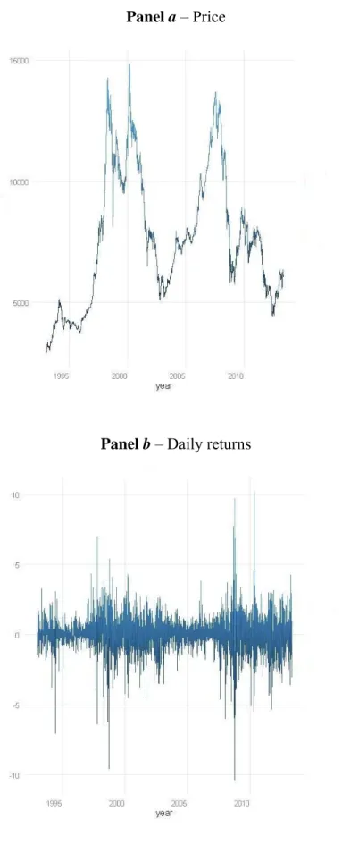
The data used to estimate the distributions consists of daily returns between December 31 1992 and May 20 2013 for the PSI-20 Index, in a total of 4.979 observations. Figure 1 shows the series with the closing price and the daily returns. We do not remove any extreme values as potential outliers from our data set, therefore market crashes and other sudden market corrections are not discarded. It would not be appropriate to remove outliers as the proper modeling of extreme returns is of great importance in risk management.

(Insert Figure 1 here)

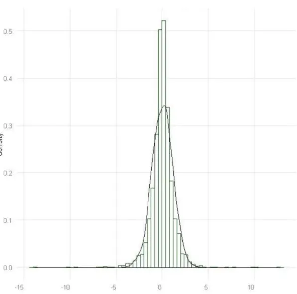
First, to get a visual impression of the shape of the daily returns density, we show in Figure 2 how the normal distribution fits this density. The actual returns are characterized by much higher kurtosis and extreme values as compared to the normal distribution.

(Insert Figure 2 here)

Second, we estimate the parameters of the normal, generalized hyperbolic, normal inverse Gaussian and Student t distributions using the procedure described in the previous section. Table 1 depicts these estimations. These parameters are then used to simulate the distributions and compare them with the actual daily returns.

(Insert Table 1 here)

In order to simulate the random variables of the distributions we use two different techniques: for the normal inverse Gaussian and Student t distributions we use

14

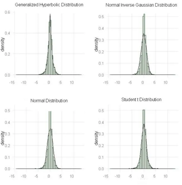
the Rydberg (1997) method, while for the generalized hyperbolic distribution we use the methodology proposed by Scott (2009). The results are depicted in Figure 3. It shows the histogram of the daily returns, superimposed with the densities of the normal, the generalized hyperbolic, the normal inverse Gaussian and the Student t distributions. We find that the generalized hyperbolic distribution closely follows the histogram of the actual daily returns, while the normal inverse Gaussian and the normal distributions have globally a lower fitting quality.

(Insert Figure 3 here)

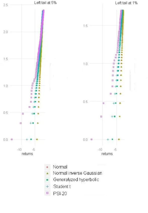
Next, we develop our study of the distributional characterizations of the Portuguese stock index by examining what is really important for risk management, namely the tail behavior of the different probability distributions. We run 4.500 simulations for each of the four distributions using the estimated parameters and then compute the average of these simulations and plot the tail behavior for a one and five percent probability levels, at both the right and left tails. In particular, we plot the log of the frequency of observations at each return for the left and right tails, as shown in Figure 4.

(Insert Figure 4 here)

We find that, in all scenarios, the density of the Student t distribution exhibits fatter tails then the other three distributions. It is closely followed by the generalized hyperbolic distribution and, at last, with less pronounced tails, we have the normal inverse Gaussian and the normal distributions. Since the Student t distribution has a marginally larger occurrence of frequency in both tails, it is the distribution that better captures the tail behavior of Portuguese stock index returns.

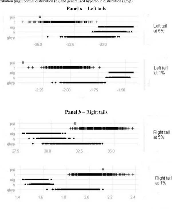
Another result that better explains the behavior of the distributions at the tails is provided by Figure 5. It shows the cumulative returns for the actual data and for the

15

simulated generalized hyperbolic, normal inverse Gaussian, normal and Student t distributions, based on 4.500 simulations. The different distributions are on the y-axis, while the simulations of the cumulative returns are on the x-axis. Panel a considers the cumulative returns at the left tails, at a five and one percent probability of the tails, whereas Panel b considers the cumulative returns at the right tails, also at a five and one percent probability of the tails. Except for the PSI-20 data which is a single data point, for all four distributions there is a range of cumulative returns at a five and one percent probability. Our aim is to examine which distribution approximates better the tails or manages to simulate returns exhibited by the actual data. We find that the Student t distribution is much better placed in capturing the cumulative returns at one and five percent probability levels, at both the right and left tails. The simulation of the generalized hyperbolic distribution also provides a good approximation of the tails, especially on the right tails. Finally, we observe that the normal inverse Gaussian and the normal distributions exhibit relatively poorer tail probabilities.

(Insert Figure 5 here)

In sum, we can say that the analysis of the tail behavior of the Portuguese stock index returns reveals that the Student t distribution provides the best approximation of the actual returns, followed by the generalized hyperbolic distribution. The average tail probability of high negative or positive returns over 4.500 simulations is higher for the Student t distribution as compared to the generalized hyperbolic distribution. The Student t distribution is important to estimate the potential loss that may be incurred on account of adverse movements in the Portuguese stock index as it would provide a better estimate of the risks. This result is in line with the findings of Markowitz and Usmen (1996a, 1996b) and Hurst and Platen (1997) who identified the Student t distribution as the best fit to daily log-return data of the S&P and other regional indices.

16

5 Conclusions

This paper investigates the fitting performance of the generalized hyperbolic, the normal inverse gaussian, the Student t and the normal distributions to the returns of the PSI-20 over the period 1992–2013. It is motivated by empirical evidence that the distribution of index returns is not Gaussian. The primary aim is to compare the density function of these distributions and to examine which one better fits the actual data for daily returns.

This paper is, as far as we are concerned, the first to examine how the returns of the Portuguese stock index conform to the density of these distributions. Initially, we compare the density function of the generalized hyperbolic, the normal inverse Gaussian and the Student t distributions to the density of the normal distribution and subsequently we analyze the tails of the distributions.

The results show that the distribution of the actual returns of the PSI-20 exhibits much higher kurtosis and extreme values as compared to the normal distribution. Furthermore, a comparison of the histogram of the daily returns with the density of the distributions reveals that the generalized hyperbolic distribution provides a very good approximation of the actual returns. This conclusion is, however, insufficient as what is really important is to study the behavior of the distributions at the tails. A more detailed analysis of the tails of the four distributions reveals that the density of the Student t distribution exhibits fatter tails then density of the other distributions. The generalized hyperbolic distribution follows the Student t distribution in terms of fitting quality at the tails and, with lower fitting quality, we find the normal inverse Gaussian and the normal distributions.

We believe the results presented in this study are of particular importance for portfolio managers who may include in their portfolios mutual funds replicating the Portuguese stock index or even derivatives associated with this index. By assuming the

17

normality of the returns in VaR analysis or other risk management decisions, not accounting for the non-normality that we have identified, portfolio managers may achieve flawed results and unreasonable estimations of portfolio returns. Future empirical research should try to apply the methodology of this paper to the returns of other European indexes, in particular of countries with similarities in terms of size and economic development with Portugal.

18

References

Abramowitz, M. and I. A. Stegun (1972). Handbook of mathematical functions with formulas, graphs, and mathematical tables. Dover, New York.

Barndorff-Nielsen, O. (1977). Exponentially decreasing distributions for the logarithm of particular size. Proceedings of the Royal Society of London, Series A, 353, 401– 419.

Barndorff-Nielsen, O. (1978). Hyperbolic distributions and distributions on hyperbolae.

Scandinavian Journal of Statistics, 5, 151–157.

Barndorff-Nielsen, O. (1995). Normal-Inverse Gaussian processes and the modeling of stock returns, Technical report, University of Aarhus.

Bauer, C. (2000). Value at risk using hyperbolic distributions. Journal of Economics

and Business, 52, 455–467.

Blattberg, R. C. and N. Gonedes (1974). A comparison of the stable and student distributions as statistical models for stock prices. Journal of Business, 47, 244– 280.

Cont, R. (2001). Empirical properties of asset returns: stylized facts and statistical issues. Quantitative Finance, 1, 223–236.

Fama, E. F. (1963). Mandelbrot and the stable paretian hypothesis, Journal of Business, 36, 420–429.

Fergusson, K. and E. Platen (2006). On the distributional characterization of daily log-returns of a world stock index. Applied Mathematical Finance, 13, 19–38.

Hurst, S. R. and E. Platen (1997). The marginal distributions of returns and volatility. In Y. Dodge (Ed.), L1-Statistical procedures and related Topics, vol. 31 of IMS

Lecture Notes – Monograph Series, 301–314. Institute of Statistics Hayward,

19

Karlis, D. (2002). An EM type algorithm for maximum likelihood estimation of the normal-inverse Gaussian distribution. Statistics and Probability Letters, 57, 43–52. Mandelbrot, B. (1963). The variation of certain speculative prices. Journal of Business,

36, 394–419.

Nelder, J. A. and R. Mead (1965). A simplex method for function minimization.

Computer Journal, 7, 308–313.

Platen, E. and R. Rendek (2008). Empirical evidence on Student-t log-returns of diversified world stock indices. Journal of Statistical Theory and Practice, 2, 233– 251.

Praetz, P. D. (1972). The distribution of share prices. Journal of Business, 45, 49–55. McNeil, A., Frey, R, and P. Embrechts (2005). Quantitative Risk Management,

Princeton University Press.

Markowitz, H. and N. Usmen (1996a). The likelihood of various stock market return distributions, Part 1: Principles of inference. Journal of Risk and Uncertainty, 13, 207–219.

Markowitz, H. and N. Usmen (1996b). The likelihood of various stock market return distributions, Part 2: Empirical results. Journal of Risk and Uncertainty, 13, 221– 247.

R Core Team (2013). R: A language and environment for statistical computing. R Foundation for Statistical Computing. Vienna, Austria

Rydberg, T. H. (1997). The normal inverse Gaussian Lévy process: Simulation and approximation. Communications in Statistics. Stochastic models 34, 887–910. Press, W. H., Teukolsky, S. A., Vetterling, W. T., and B. P. Flannery (1992). Numerical

Recipes in C. Cambridge University Press.

20

Fig. 1 Price and daily returns of the Portuguese Stock Index (PSI-20) from 31/12/1992 to 20/05/2013

Panel a – Price

21

22

23

Fig. 4 Tails at 5% and 1% for the actual daily returns of PSI-20 and normal, normal inverse Gaussian, generalized hyperbolic and Student t distributions

24

25

Fig. 5 Cumulative returns at 5% and 1% for the actual daily returns and the distributions We use the following notation: Portuguese stock index (psi); Student t distribution (t); normal inverse Gaussian distribution (nig); normal distribution (n); and generalized hyperbolic distribution (ghyp).

Panel a – Left tails

26

Table 1 Estimated parameters of the distributions

Panel a – Normal distribution

µ σ

Normal

distribution 0,014214 1,165586

Panel b – Generalized hyperbolic, normal inverse Gaussian and Student t distributions

Maximum Likelihood value λ α β δ µ Generalized hyperbolic distribution -2.596,24 1,0 1,3 0,0001166 0,00002 0,014214 Normal inverse Gaussian distribution -13.217,41 -1/2 0,583217 -0,042927 0,757655 0,070133 Student t distribution -7.093,39 2,0 0 0 2,44949 0,014214