HOLOS, Ano 35, v.1, e7393, 2019 1
DRAG COEFFICIENT AND MODELING THE VERTICAL WIND PROFILE IN FORESTS
A. B. SANTOS1, J. TOTA2, A. M. D. ANDRADE2 e R. G. CARNEIRO3 Federal University of Rio Grande do Norte1 , Federal University of Western Pará2 ,
National Institute for Space Research3 [email protected]
Artigo submetido em 13/06/2018 e aceito em 23/06/2019 DOI: 10.15628/holos.2019.7393
ABSTRACT
The difficulties in modeling and determining important parameters, for example, drag coefficient for the flows in forests are themes of many researches that try to rescue the classic approaches and to clarify some aspects present in the literature. Based on this, an analytical one-dimensional model was developed to describe the drag coefficient profile within canopy using average wind
speed above the canopy and the leaf area density. The model managed to satisfactorily represent the drag coefficient profile and the comparative analysis indicates that the empirical drag coefficient profile is similar the inferred profile, suggesting that the model can be an alternative to be used in parameterization and understanding of the wind-canopy interactions.
KEYWORDS: Canopy, wind speed, drag coefficient, leaf area density.
COEFICIENTE DE ARRASTO E MODELAGEM DO PERFIL VERTICAL DO VENTO EM
FLORESTAS
RESUMO
As dificuldades em modelar e determinar parâmetros importantes, por exemplo, o coeficiente de arrasto para os fluxos em florestas são temas de muitas pesquisas que tentam resgatar as abordagens clássicas e esclarecer alguns aspectos presentes na literatura. Com base nisso, um modelo unidimensional analítico foi desenvolvido para descrever o perfil do coeficiente de arrasto dentro do dossel usando a velocidade média do vento acima do
dossel e a densidade da área foliar. O modelo conseguiu representar satisfatoriamente o perfil do coeficiente de arrasto e a análise comparativa indica que o perfil do coeficiente de arrasto empírico é semelhante ao perfil inferido, sugerindo que o modelo pode ser uma alternativa a ser utilizada na parametrização e compreensão das interações vento-copa.
HOLOS, Ano 35, Vol. 01 2
1 INTRODUCTION
Several experimental studies have helped to formulate an understanding of the processes of heat, mass and momentum changes between the vegetation and the atmosphere (Thom 1971; Fitzjarrald et al. 1988; Shaw et al. 1988; Fitzjarrald et al. 1990a; Fitzjarrald et al. 1990b; Tóta et al. 2008, 2012; Santos et al. 2013; Oliveira et al. 2013; Santos et al. 2016; Dias-Junior et al. 2017). Contributing to improve the terrestrial surface parameterizations of numerical weather forecasting models (e.g. Kaimal and Finnigan 1994; Belcher and Hunt 1998;Belcher et al. 2012; Xu et al. 2017) and the development of different models of turbulence based on empirical relations or involving solutions of the momentum equation using closing techniques that investigate the structure of air flow over forests (Shaw 1977; Wilson & Shaw, 1977; Katul et al., 2004;Yi et al. 2005; Yi 2008; Xu et al. 2013, 2015; Sousa et al.2016; Santana et al. 2017).
Therefore, knowledge of this structure is necessary for a better understanding of the impact that vegetation elements such as leaves, branches and trunks cause in the field of wind and in the transport of mass, energy and momentum. According to some studies (see Wilson e Shaw 1977; Raupach et al. 1996; Finnigan 2000) vegetation interacts with and influences the wind flow of the lowest atmospheric layers as follows: 1) In extracting momentum from the flow due to the aerodynamic drag of the plant parts; 2) In converting kinetic energy of the mean flow into turbulent kinetic energy in the wakes formed behind obstructions to the flow; 3) in breaking down large-scale turbulent motions into smaller large-scale motions, again in the wake flow. It is known that the vegetative elements are an obstruction to the flow of the air that undergoes a deceleration due to the action of the drag force which creates velocity gradients and e eddies resulting in the loss of momentum of the fluid, that is, the set of vegetative elements forms a rough surface that when it interacts with the air flow changes its dynamic behavior, making it difficult to model this phenomenon (see Wilson e Shaw 1977; Shaw 1977; Raupach et al. 1996; Finnigan 2000; Yi et al. 2005; Yi 2008).
It is clear that one of the main limitations in the application of turbulent closure models to the canopies of the plants is the descriptions of the architectural characteristics, aerodynamics and the absorption of momentum. These difficulties in modeling and determining important parameters for the flow in forests are themes of many researches that try to rescue the classic approaches and to clarify some aspects present in the relevant literature. For example, Yi (2008) in order to understand the transfer of canopy momentum postulated three new hypotheses that combined the momentum equation established the relationship between the observed S-shaped wind profile and the exponential flux profile within forest canopies. With this, the author was able to obtain empirically and directly the profile of drag coefficient from observed profiles of wind speed and Reynolds stress, also could deduce from theoretical predictions substituting terms into the momentum equation.
However, this new method encounters the difficulty of obtaining vertical wind profile data in forests. Based on this, the purpose of the present study is test a simple analytical model for drag coefficient profile using average wind speed above the canopy and the leaf area density.
HOLOS, Ano 35, Vol. 01 3
2 MATERIAL AND METHOD
2.1 Data
Observed data used in this study were taken from the literature (Amiro 1990). The experiments were conducted by Amiro 1990 in three different boreal forest canopy sites in southeastern Manitoba, Canada. The profiles were measured by two triaxial sonic anemometers: one operated above the forest canopy while the other was roving at different heights at the spruce site were 12.1, 9.2, 6.2, 4.2, and 1.8 m; at the jack pine site 17, 13.1, 8.7, 5.8 and 1.9 m; and at the aspen site 13.1, 8.7, 5.8, 3.4 and 1.4 m.
Amiro 1990, estimated the height of the canopy top (h) to be about 15 m for the pine canopy, and 10 m for the spruce and aspen canopies and your best estimates of total leaf area index (LAI) are about 10 for the spruce canopy, 4 for the aspen canopy, and 2 for the pine canopy. All sites are natural plant canopies and only small paths were created for access to the experimental area (See table 2 and for more details see Amiro 1990).
Table 1: Canopy morphology.
Canopy Aspen Spruce Pine
h (m) 10 10 15
LAI (m2 m-3) 4 10 2
2.2 Methods
2.2.1 Drag force
The mathematical expression for the drag force created by canopy elements is most commonly expressed by
F = ρCDau̅2 (1)
Where ρ is air density, CD an effective drag coefficient for the plant parts (the factor 1 2⁄ is
absorbed in CD following the micrometeorological convention), a the plant area density and u̅ the
mean wind speed.
The drag coefficient within the canopy (CD(z)) can be determined empirically, and directly, from observed profiles of wind speed and Reynolds stress. According to Mahrt et al. (2000) can be defined as
CD(z) =
u∗2(z)
u2(z) (2)
HOLOS, Ano 35, Vol. 01 4
−u̅̅̅̅̅̅ = u′w′ ∗
2(z) (3)
Where −u̅̅̅̅̅̅ is the average shear stress. ′w′
2.2.2 Alternative method to the estimate of the drag coefficient
If the normalization profiles of wind speed and cumulative leaf area are the same between two systems, the relative distribution of the drag coefficient differs only by LAI. Therefore, an alternative method to the estimate of the drag coefficient is proposed considering a dependence on the LAI profile, thus,
CD(z) = CDh + (a(z) β⁄ )exp {− [1 −
z
h]} (4)
or
CD(z) =u̅̅̅̅̅̅(h)′w′
u̅h2 + (a(z) β⁄ )exp {− [1 −
z
h]} (5)
Where h is top of canopy and β is fit parameter of the equation to the observed data.
From now on this method to the estimate of the drag coefficient will be called Santos Model.
2.2.3 Vertical wind profile
To understand the basic characteristics of the wind profile and the exponential flux profile within forest canopies Yi (2008) proposed new hypotheses that establish the relationship between the mean wind speed and Reynolds stress. These hypotheses are 1) within the canopy, the transport of horizontal momentum is continuous and downward. Meanwhile the horizontal momentum is continuously absorbed by canopy elements from the air; 2) a local equilibrium exists between the rate of horizontal momentum transfer and its rate of loss and 3) the drag coefficient is equivalent whether defined in the local equilibrium relationship or defined in the volumetric drag force in the momentum equations, if their averaging operations are the same. From these hypotheses the wind speed profile was characterized as follows:
u̅(z) = u̅h[CDh⁄CD(z)]1/2exp{−0.5[LAI − L(z)]} (6)
Where CDh and u̅h are the respective drag coefficient and mean wind speed at the top of the
canopy. Where LAI is the leaf area index and [LAI − L(z)] is the cumulative leaf area between z and the top of canopy, and L(z) is the cumulative leaf area between the ground and z is defined as
L(z) = ∫ a(zz ′)dz′
HOLOS, Ano 35, Vol. 01 5
2.2.4 Statistic analyze
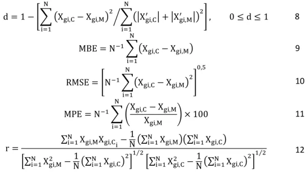
The models performances were evaluated by comparing their estimates with the respective values measured in the field from five statistical indexes: Willmott's concordance index (d) (Eq. 8) determines the accuracy of the method and indicates the degree of distance from the estimated to the observed values. This index varies from 0, no agreement, to 1, perfect concordance, MBE (Mean Bias Error) (Eq. 9) that evaluates if the model overestimates or underestimates the observed values, RMSE (Root Mean Square Error) (Eq. 10) whose objective is to show the size of the given estimate error. It should be noted that the zero value is a perfect indicates, but this estimated and measured values increases difference between, MPE (Mean Percentage Error) (Eq. 11) and and the Pearson’s correlation coefficient (r) (Eq. 12) (Willmott 1982, Wilks 2011, Khorasanizadeh e Mohammadi 2013): d = 1 − [∑ (Xgi,C− Xgi,M) 2 ∑(|Xgi,C′ | + |X gi,M′ |) 2 N i=1 ⁄ N i=1 ] , 0 ≤ d ≤ 1 8 MBE = N−1∑(X gi,C− Xgi,M) N i=1 9 RMSE = [N−1∑(X gi,C− Xgi,M)2 N i=1 ] 0,5 10
MPE = N−1∑ (Xgi,C− Xgi,M
Xgi,M ) N
i=1
× 100 11
r = ∑ Xgi,MXgi,Ci− 1N (∑ Xgi,M
N
i=1 )(∑Ni=1Xgi,C) N i=1 [∑ Xgi,M2 − 1 N (∑Ni=1Xgi,C) 2 N i=1 ] 1 2⁄ [∑ Xgi,C2 − 1 N (∑Ni=1Xgi,C) 2 N i=1 ] 1 2⁄ 12
Where Xgi,C é is the nth variable estimated or calculated by the model Xgi,M is the nth measured
variable, Xgi,C′ = Xgi,C− X̅gi,M e Xgi,M′ = Xgi,M− X̅gi,M, e X̅gi,M is the mean of the measured values.
3 RESULTS
In this section, theoretical predictions are compared with the observations using previously published data for canopies with nonuniform vertical leaf area distributions.
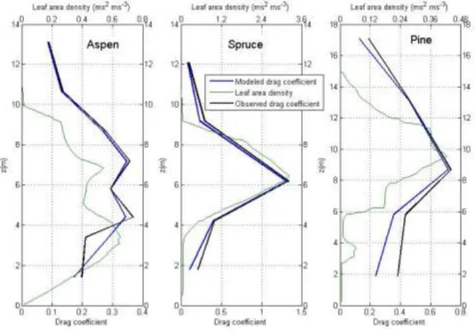
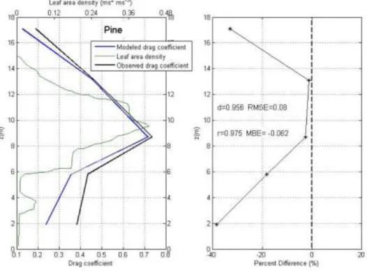
Figure 1 shows the comparison between drag coefficients estimated by Equation (4) and observed data for the three canopy types. The drag coefficients above the canopy (CDh) calculated for each forest are 0.13 for the Pine, 0.086 for the Spruce and 0.087 for the aspen close to the value 0.2 adopted by Massman (1997) and agreeing with the results (CDh in the range 0.15–0.25) presented in Marcolla et al. (2003) and with the range 0.12–0.19 of that was observed for a coniferous forest at Lavarone in Italy by Cescatti and Marcolla (2004). Shaw et al. (1988) found drag coefficients on the order of 0.1 at the canopy top. The magnitudes of the local drag
HOLOS, Ano 35, Vol. 01 6
coefficients predicted here are within the ranges observed by Brunet et al. (1994) in wind tunnel experiments for terrestrial canopies (0–2). The Santos model was able to reproduce satisfactorily the observed drag coefficient profile with a slight underestimation
It is verified the profiles of leaf area density and of drag coefficients are quite similar and maximum drag coefficients are located around the maximum leaf area density levels for three forest canopies. The drag coefficient increases dramatically as the increases leaf area density reaching the value of 0.74 for the Pine(between 8 and 10 m and maxima foliar density of 0.43 m2
m-3), 1.34 for the Spruce (between 6 and 8 m and maxima foliar density of 3.22 m2 m-3) and 0.37
for the Aspen (between 2 and 6 m and maxima foliar density of 0.65 m2 m-3). This increase is due
to the complex array of leaves, branches and other components of forest canopies create resistance to the air flows.
Figure 1: Comparison of predicted drag coefficient profiles from the Santos model (solid blue line) to observed data (solid black line)in three vegetation types (see Table 1). The observed drag coefficients were calculated by Eq. (2) from the observed data of wind speed and Reynolds stress reported in the literature (Amiro 1990). The solid gray line is leaf area density profile.
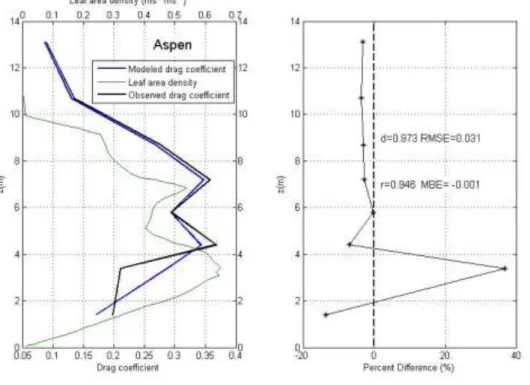
The performance of the model was evaluated by comparing their estimates with their respective values measured on site by five statistical indexes (as shown in Fig. 2-4). Figure 2 shows the percent difference between the modeled and observed at different heights for the Aspen site. The result show that the model has satisfactory performance with Willmott's concordance index (d) of 0.973 and the Pearson’s correlation coefficient (r) of 0.946 and presented Root Mean Square Error (RMSE) that gives the standard deviation of the model prediction error of 0.031. The smaller value indicates better model performance. The percent difference shows the average tendency of the simulated values to be larger or smaller than their observed ones. It was observed that the model underestimated the drag coefficient values on layer between z=4 and z=14 with a difference
HOLOS, Ano 35, Vol. 01 7
about 10% and overestimated the values on layer between z=2 and z=4 with a difference about 20%. On average the model underestimated the drag coefficient values with a mean bias error (MBE) of -0.001.
Figure 2: Statistical indexes and percent difference between the modeled and observed for the Aspen site.
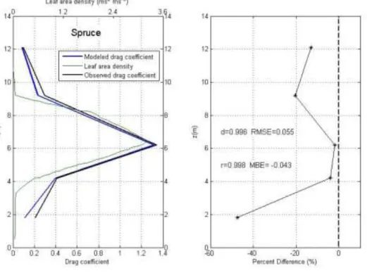
Figure 3 exhibit the percent difference between the modeled and observed at different heights for the Spruce site. It was noticed that the model has excellent performance with d=0.996 and r=0.998 and RMSE=0.055 that gives the standard deviation of the model prediction error and the lower the value better model performance.
The percent difference shows that the model underestimated the drag coefficient values on layer across the layer with a greater difference about 40% between z=0 and z=2. On average the model underestimated the wind velocity values with a MBE of -0.043.
HOLOS, Ano 35, Vol. 01 8
Figure 3: Statistical indexes and percent difference between the modeled and observed for the Spruce site.
Figure 4 presented the percent difference between the modeled and observed at different heights for the Pine site. It was verified that the model has satisfactory performance with d=0.956 and r=0.975 and presented Root Mean Square Error of 0.08. The percent difference showed that the model underestimated the drag coefficient values across the layer with a greater difference about 40% between z=0 and z=2. On average the model underestimated the drag coefficient values with a MBE=-0.062.
In the three experimental sites the Santos model was able to reproduce satisfactorily the observed drag coefficient profile with a slight underestimation. The comparative analysis indicates that the empirical drag area profile is similar the inferred profile, suggesting that the Santos model can be an alternative to be used in parameterization and understanding of the wind-canopy interactions.
HOLOS, Ano 35, Vol. 01 9
Figure 4: Statistical indexes and percent difference between the modeled and observed for the Pine site.
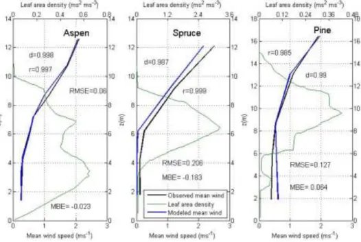
The drag coefficient profile estimated was used to calculate wind speed profile and results were presented in Figure 5 with experimental data for comparison and statistical indexes. The predicted wind speed profile is in good agreement with the observed profile. The model predicts a decrease in the wind speed within the layer of maximum leaf area density the foliage extracts momentum from the flow through drag forces, and reaches a minimum on the lower side of this layer. In Aspen this minimum was less than 12% of its value above the canopy and 28% in pine and 0.7% in spruce this implying that majority all momentum of the above wind flow is absorbed by the crown layer. It was noted the shape of the wind profile is determined by the flow resistance properties of canopy structure, i.e., the drag area of plant elements and associated drag coefficient.
It was observed that the model has excellent performance with d=0.998 and r=0.997 for Aspen, d=0.987 and r=0.999 for Spruce and d=0.99 and r=0.985 for Pine and presented RMSE that gives the standard deviation of the model prediction error of 0.06 for Aspen, 0.206 for Spruce and of 0.127 for Pine. The smaller value indicates better model performance. On average the model underestimated the wind velocity values with a mean bias error (MBE) of -0.023 ms-1for Aspen and
-0.183 ms-1 for Spruce, while the model overestimated values with a mean bias error (MBE) of
HOLOS, Ano 35, Vol. 01 10
Figura 5: Comparison between the observed wind speed profile (black line) and estimated by Eq. (6) using drag coefficient data estimated by Santos model.
4 CONCLUSIONS
In this work, an alternative method is presented to calculate the drag coefficient profile using average wind velocity above the canopy and the leaf area index. This method is an empirical-analytical model which provides a general non-dimensional relationship. It is known that the drag coefficient is an important parameter which links canopy architecture with its aerodynamic behavior. The results presented in the previous section show that the Santos model managed to satisfactorily represent the observed drag coefficient profile with a slight underestimation for three forests. Predictions of maximum drag coefficient were located around the maximum leaf area level for three forests. The estimated drag coefficient by model was used to calculate the vertical wind speed profile. The vertical wind speed profile model predictions were realistic and satisfactory when tested against the observed data of three forests.
Acknowledgments
The first author acknowledges the financial support of the Ministry of Education and Coordination of Higher Education and Personnel Training (CAPES), through the Foundation for Research Support of Rio Grande do Norte, for the PhD Scholarship grants.
HOLOS, Ano 35, Vol. 01 11
5 REFERÊNCIAS
Amiro, B. D. (1990). Comparison of turbulence statistics within three boreal forest canopies.
Boundary Layer Meteorology, 51, 99–121.
Belcher, S. E. & Hunt, J. C. R. (1998). Turbulent flow over hills and waves. Annual Review of Fluid
Mechanics, 30(1), 507-538.
Belcher S., Harman I. & Finnigan J. (2012). The wind in the willows: flows in forest canopies in complex terrain. Annual Review Fluid Mechanics, 44, 479–504.
Brunet, Y., Finningan, J., & Raupach, M. (1994). A wind tunnel study of air flow in waving wheatsingle point velocity statistics. Boundary Layer Meteorology, 70, 95–132.
Cescatti, A. & Marcolla, B. (2004). Drag Coefficient and Turbulence Intensity in Conifer Canopies
Agricultural and Forest Meteorology, 121, 197-206.
Dias-Júnior, C. Q., Sá, L. D., Marques Filho, E. P., Santana, R. A., Mauder, M. & Manzi, A. O. (2017). Turbulence regimes in the stable boundary layer above and within the Amazon forest.
Agricultural and Forest Meteorology, 233, 122–132.
Finnigan J. (2000). Turbulence in plant canopies. Annual Review of Fluid Mechanics, 32, 519–571. Fitzjarrald, D. R., Moore, K. E., Cabral, O. M. R., Scolar, J., Manzi, A. O. & Abreu Sá, L. D. (1990a). Daytime turbulent exchange between the Amazon forest and the atmosphere, Journal of
Geophysical Research: Atmospheres, 95(10), 16–838.
Fitzjarrald, D. R. & Moore, K. E. (1990b). Mechanisms of nocturnal exchange between the rain forest and the atmosphere, Journal of Geophysical Research, 95(10), 16839–16850.
Fitzjarrald, D. R., Stormwind, B. L., Fisch, G. & Cabral, O.M. R. (1988). Turbulent transport observed just above the Amazon forest, Journal of Geophysical Research, 93(2), 1551–1563.
Kaimal, J. C. & Finnigan, J. J. (1994). Atmospheric Boundary Layer Flows, Oxford University Press, New York, EUA, 289 pp.
Katul, G. G, Mahrt, L., Poggi, D. & Sanz, C. (2004). One and Two Equation Models for Canopy Turbulence. Boundary Layer Meteorology, 113, 81-109
Khorasanizadah, H. & Mohammadi, K. 2013. Introducing the best model for predicting the monthly mean global solar radiation over six major cities of Iran. Energy, 51, 257-266.
Marcolla, B., Pitacco, A. & Cescatti, A. (2003). Canopy architecture and turbulence structure in a coniferous forest. Boundary Layer Meteorology, 108, 39–59.
Mahrt, L., Lee, X., Black, A., Neumann, H. & Staebler, R. M. (2000). Nocturnal mixing in a forest subcanopy. Agricultural and Forest Meteorology, 101, 67–78.
Massman, W. J. (1997). An analytical one-dimensional model of momentum transfer by vegetation of arbitrary structure. Boundary Layer Meteorology, 83, 407–421.
HOLOS, Ano 35, Vol. 01 12
Oliveira, P. E. S., Acevedo, O. C., Moraes, O. L. L., Zimmermann, H. R. & Teichrieb, C. (2013). Nocturnal intermittent coupling between the interior of a pine forest and the air above it.
Boundary Layer Meteorology, 146, 45–64.
Raupach, M.R., Finnigan, J.J. & Brunt, R. (1996). Coherent eddies and turbulence in vegetation canopies the mixing-layer analogy. Boundary Layer Meteorology. 78, 351-382.
Santana, R. A. S., Dias-Junior, C. Q., Val, R. S. D., Tota, J. & Fitzjarrald, D. R. (2017). Observing and Modeling the Vertical Wind Profile at Multiple Sites in and Above the Amazon Rain Forest Canopy, Advances in Meteorology, http://dx.doi.org/10.1155/2017/5436157, Article ID 5436157, 8 pages.
Santos, A. B., Tóta, J., Moura, M. A. L., Fitzjarrald, D. R., Santana, R. A. S., Andrade, A. M. D. & Carneiro, R. G. (2013). Dinâmica do Escoamento de Ar Acima e Dentro de uma Floresta Tropical Densa sobre Terreno Complexo na Amazônia. Revista Brasileira de Geografia Física, 6(2), 308– 319.
Santos, D. M., Acevedo, O. C., Chamecki, M., Fuentes, J. D., Gerken, T. & Stoy, P. C. (2016). Temporal Scales of the Nocturnal Flow Within and Above a Forest Canopy in Amazonia, Boundary Layer
Meteorology, 161, 73–98, doi:10.1007/s10546-016-0158-5,
Shaw, R. H. (1977). Secondary wind speed maxima inside plant canopies. Journal of Applied
Meteorology, 16, 514–521.
Shaw, R. H., Den Hartog, G. & Neumann, H. H. (1988). Influence of foliar density andthermal-stability on profiles of Reynolds stress and turbulence intensity in adeciduous forest. Boundary
Layer Meteorology, 45, 391–409.
Souza, C. M., Dias-Júnior, C. Q., Tóta, J., & Abreu Sá, L. D. (2016). An empirical-analytical model of the vertical wind speed profile above and within an Amazon forest site. Meteorological
Applications, 23(1), 158–164.
Thom, A. S. (1971). Momentum absorption by vegetation. Quarterly Journal of the Royal
Meteorological Society, 97, 414–428.
Tóta, J., Fitzjarrald, D. R., Staebler, R. M., Sakai, R. K., Moraes, O. L. L., Acevedo, O. C., Wofsy, S. C. & Manzi, A. (2008). Amazon rain forest subcanopy flow and the carbon budget: Santarem LBA-ECO site, Journal of Geophysical Research: Biogeosciences, 113, doi:10.1029/2007JG000597. Tóta, J., Fitzjarrald, D. R. & da Silva Dias, M. A. F. (2012). Amazon rainforest exchange ofcarbon and subcanopy air flow: manaus LBA site-a complex terrain condition. The Scientific World
Journal, 165067, http://dx.doi.org/10.1100/2012/165067.
Wilks D. S. (2011). Statistical methods in the atmospheric sciences. 3rd Ed, Academic, New York,
676 pp.
Willmott C. J. (1982). Some comments on the evaluation of model performance. Bulletin of the
HOLOS, Ano 35, Vol. 01 13
Wilson, N. R. & Shaw, R. H. (1977). A higher order closure model for canopy flow. Journal of Applied
Meteorology, 16, 1197–1205.
Xu, X. & Yi, C. (2013). The influence of geometry on recirculation and CO2 transport over forested
hills. Meteorology and Atmospheric Physics, 119, 187–196.
Xu, X., Yi, C. & Kutter, E. (2015). Stably stratified canopy flow in complex terrain. Atmospheric
Chemistry and Physics, 15, 7457–7470.
Xu, X., Yi, C., Montagnani, L. & Kutter, E. (2017). Numerical study of the interplay between thermo-topographic slope flow and synoptic flow on canopy transport processes. Agricultural and
Forest Meteorology.http://dx.doi.org/10.1016/j.agrformet.2017.03.004
Yi, C., Monson, R. K., Zhai, Z., Anderson, D. E., Lamb, B. Allwine, G., Turnipseed, A. A. & Burns, S. P. (2005). Modeling and measuring the nocturnal drainage flow in a high-elevation, subalpine forest with complex terrain. Journal of Geophysical Research, 110, D22303, doi:10.1029/2005JD006282.
Yi, C. (2008). Momentum transfer within canopies. Journal of Applied Meteorology and