Ana Margarida Barradinhas da Silva

(1)

Ana Margarida Barradinhas da Silva

Licenciatura em Ciências de Engenharia do Ambiente

Heat Recovery from Wastewater:

Numerical Modelling of Sewer Systems

Dissertação para obtenção do Grau de Mestre em

Engenharia do Ambiente, perfil Engenharia Sanitária

Orientadora:

Professora Doutora Leonor Monteiro do Amaral

Professora Auxiliar, FCT/UNL

.Jurí:

..Presidente e Arguente: Prof. Doutor Pedro Manuel Hora Santos Coelho

Vogal: Prof. Doutor António Pedro de Coimbra Macedo Mano

Vogal: Prof. Doutora Leonor Miranda Monteiro do Amaral

(2)

(3)

Ana Margarida Barradinhas da Silva

Licenciatura em Ciências de Engenharia do Ambiente

Heat Recovery from Wastewater:

Numerical Modelling of Sewer Systems

Dissertação para obtenção do Grau de Mestre em

Engenharia do Ambiente, perfil Engenharia Sanitária

Orientadora:

Professora Doutora Leonor Monteiro do Amaral

Professora Auxiliar, FCT/UNL

.Jurí:

..Presidente e Arguente: Prof. Doutor Pedro Manuel Hora Santos Coelho

Vogal: Prof. Doutor António Pedro de Coimbra Macedo Mano

Vogal: Prof. Doutora Leonor Miranda Monteiro do Amaral

(4)

(5)

v

Heat Recovery from Wastewater: Numerical Modelling of Sewer Systems

A Faculdade de Ciências e Tecnologia e a Universidade Nova de Lisboa têm o direito,

perpétuo e sem limites geográficos, de arquivar e publicar esta dissertação através de

exemplares impressos reproduzidos em papel ou de forma digital, ou por qualquer outro

meio conhecido ou que venha a ser inventado, e de a divulgar através de repositórios

científicos e de admitir a sua cópia e distribuição com objectivos educacionais ou de

investigação, não comerciais, desde que seja dado crédito ao autor e editor.

(6)

(7)

vii

Acknowledgments/ Agradecimentos

I would like to thank to Jorge Maxil (TU Delft), Dr Jan Hofman (KWR), Dr Mirjam Blokker

(KWR) and Dr Luuk Rietveld (TU Delft). I am very grateful to Dr Bas Wols (KWR) to

support me.

To all my friends in the Netherlands thank you. Nevertheless some of them should be

mentioned due to their true friendship and support:

Maria Lascas and Bruno Gracio, to be my second family in the Netherlands and to treat me

like their younger sister with the right to have a special room in their home.

To Diana Brandão and Maria Lousada Ferreira for integrate me in TU Delft, Delft life and

for their true friendship.

To Shirin Malekpour and Eveline van Amstel for their friendship and encouragement every

day.

Aos professores da FCT/UNL que contribuíram para a minha formação.

À Professora Doutora Leonor Amaral pela sua amizade, apoio, motivação, orientação e

por tornar este projecto possível.

A todos os meus amigos que durante estes cinco anos de Faculdade me apoiaram e que

contribuíram directa ou indirectamente para a realização deste trabalho. Algumas destas

pessoas devem ser mencionadas:

À Vanessa Tavares, por toda a amizade demonstrada e por ter sido sempre uma presença

constante.

À Diana Garcia, grande amiga e companheira de casa que muito me aturou.

À Susana Inocêncio, companheira de Guerra, que muito me ajudou e me fez não

desesperar.

À Marta Alves, Ana Rodrigues, Sandra Gonçalves, Mariana Marques e Luís Ramos por

todo o apoio e amizade. E claro, ao João Martins e João Wang pelos conselhos ao longo

do curso e amizade.

À Marta Brito, por todo o carinho e interesse que sempre demonstrou ao longo destes

anos.

À Helena Graça, Catarina Cravo, Marta Ramalho, Mariana Soares, Inês Crujo, Joana

Correia, Marlene Soares, Miguel Fitas, Miguel Jeremias, Hugo Medeiros, Miguel Curado,

João Oliveira, Luís Cabecinha e João Santos pela amizade e grande carinho.

À minha gata Nabiça pela companhia neste últimos anos, nunca me deixando estudar

(8)

viii

Ao grupo de dança contemporânea Modernus, à casa Largo do Andaluz, à República

Manjerigata e à Casinha da Vanessa por me acolherem.

Por fim, o meu maior agradecimento é para aqueles que mais amo. Aos meus pais, irmão

e namorado. Aos meus pais por me apoiarem sempre e fazerem do impossível possível.

Ao meu namorado pela dedicação e paciência neste anos de Faculdade e nomeadamente

no período da Tese. Dedico assim este trabalho aos meus pais, André e à memória dos

(9)

(10)

(11)

xi

Resumo

Este trabalho enquadra-se num projecto desenvolvido numa colaboração entre a

Universidade Técnica de Delft (TU Delft) com a empresa Waternet e KWR. Pretende-se

estudar a viabilidade do aproveitamento de energia térmica associada as águas residuais

e assim reduzir as emissões de dióxido de carbono (CO2) associadas ao sector

energético. O presente trabalho parte de um modelo computacional previamente

desenvolvido que simula recuperação de calor proveniente de águas residuais para casos

de caudal e temperatura constante.

Um dos objectivos pretende simular uma descarga de águas residuais. Para tal e por

forma a torná-los variáveis, foi adicionada uma função Gaussiana às condições de

fronteira da temperatura da água e caudal. Como segundo objectivo, pretende-se

determinar a importância dos termos presentes na equação de balanço de calor na água e

na equação de balanço de calor no ar. Para isso, introduziram-se coeficientes binários por

cada termo destas equações e processaram-se os sistemas resultantes das combinações

possíveis.

Simulou-se com sucesso uma descarga principal para a situação variável, as previsões

numéricas para a temperatura da água e caudal foram apresentadas. Quanto à avaliação

dos termos nas duas equações em questão, conclui-se que os termos fluxo de calor tubo –

água (!!") e fluxo de calor tubo – ar (!!") apresentam ser fulcrais no balaço de calor na

água e ar, respectivamente. Com o intuito de reduzir oscilações indesejadas o dt foi

reduzido, verificando-se uma diminuição das oscilações, bem como uma variação na

altura de água na tubagem que não tinha sido verificada até agora.

Este trabalho culmina assim com uma secção de desenvolvimentos futuros por forma a

melhorar os resultados obtidos. Apesar do estado actual destas rotinas não permitir uma

avaliação precisa das trocas de calor em tubagens, os resultados obtidos são bastante

promissores. Provando-se que a modelação numérica de recuperação de calor contribuirá

para o desenvolvimento do projecto principal.

(12)

(13)

xiii

Abstract

This thesis was carried as a collaboration of Delft University of Technology (TU Delft) and

the companies Waternet and KWR. The main project aims to study the possibility of

thermal energy recovery from wastewater, reducing the carbon dioxide (CO2) emissions

linked to the energy sector. The present work is based on a previous computational model

that was developed to simulate heat recovery from wastewater for constant flow rate and

temperature of water.

The first goal is to simulate a wastewater discharge. In order to achieve this, a Gaussian

function was added to the boundary conditions for water flow rate and water temperature.

As a second goal, this work aims to assess the significance of the terms present in the

water heat balance and air heat balance equations. Binary coefficients were added in each

term of both equations and then all the combinations were computed.

The unsteady situation successfully simulated a main discharge and numerical predictions

for water temperature and flow rate are presented. The deviations associated with the

modified cases for the two equations suggest that the heat flux pipe to water (!!") and

heat flux pipe to air (!!") terms are crucial for water and air heat balance predictions, respectively. In order to smooth extra oscillations, the time step (dt) was reduced and a

smaller relative size of oscillations was obtained.

This work concludes with a section of future developments in order to improve the results

obtained. Despite of the fact that the current state of these routines does not allow us to

accurately assess heat exchanges in pipes, promising results were obtained, proving that

numerical modelling of heat recovery will contribute greatly to the development of the main

project.

(14)

(15)

xv

List of figures

Figure 2.1: Open-Channel flow nonuniform flow.. ... 8

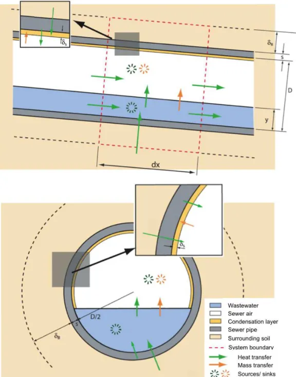
Figure 2.2: Schematic representation of a sewer pipe. In the upper view a control volume

is defined (red dashed outline) and five compartments: “sewage”, “sewer air”,

“condensation layer”, located “pipe wall” and “soil”. The lower view is a section through

this control volume with transfer processes: orange arrows indicate mass transfer and

green arrows denote heat transfer. ... 10

Figure 3.1: Representation of model structure with the seven fields: constant conditions (cond), constants (const), conditions of pipe (pipe), numerics (num), conditions of the

network (line), stationary solution (stat) and results data (data). ... 20

Figure 3.2: Example for a data cell with Tw_and_Qw_{as fields. ... 24}

Figure 3.3: Previously developed program in MATLAB® in KWR Water Research Institute

(Nieuwegein, The Netherlands) by Bas Wols, containing 3 functions: fun_start,

sewer_temp_main and fun_plot. Number of steps defined by the user. ... 26

Figure 3.4: A Gaussian function (f) starts at t0_{over the numerical time}tn_{, the duration of}

the discharge is tL_{and the peak has amplitude}_A_{. ... 28}

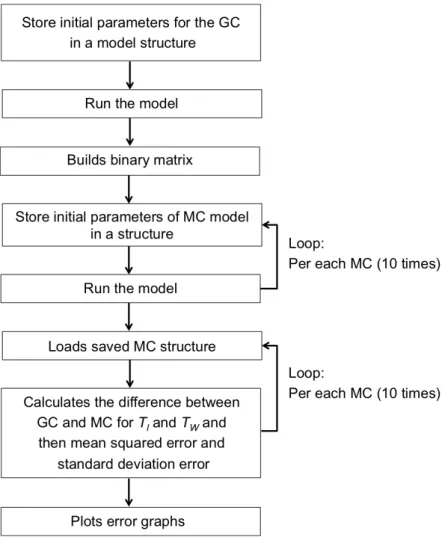
Figure 3.5: Developed model in MATLAB® with the principal phases. ... 29

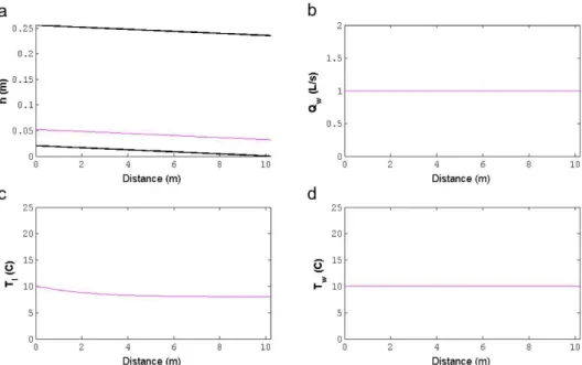
Figure 4.1: Representation in position of the pipe water depth (h) (4.1a), water flow rate (Qw) (4.1b), air temperature (Tl) (4.1c) and water temperature (Tw_{) (4.1d), for a steady}

situation of the general case. Line colour denotes different time instants (five times

depicted, however coincidental). ... 36

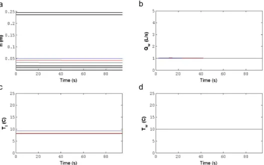
Figure 4.2: Representation in time for unsteady situation and general case for three positions in the pipe, x=1m in blue, x=5_m_{in red and}_x₌10_m_{in black: water depth}

(h) (4.2a), water flow rate (Qw) (4.2b), air temperature (Tl) (4.2c) and water

temperature (Tw_{) (4.2d). ... 37}

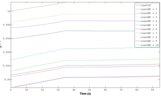
Figure 4.3: Water temperature (Tw_{) over the time for a fixed length}_x₌10_m_{. Each line}

represents the 10 modified cases for steady situation. ... 38

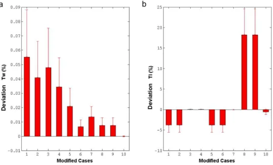
Figure 4.4: Difference between the general case and each modified case for the water temperature (Tw_{) (4.4a) and air temperature (}_Tl_{) (4.4b) and than the mean and the}

standard deviation. Steady situation. ... 39

Figure 4.5: Representation in position of the pipe water depth (h) (4.5a), water flow rate (Qw) (4.5b), air temperature (Tl) (4.5c) and water temperature (Tw_{) (4.5d), for an}

unsteady situation of the general case. Line colour denotes different time instants (five

(18)

xviii

Figure 4.6: Representation in time for unsteady situation and general case for three positions in the pipe, x=1m in blue, x=5_m_{in red and}_x₌10_m_{in black: water depth}

(h) (4.6a), water flow rate (Qw) (4.6b), air temperature (Tl) (4.6c) and water

temperature (Tw_{) (4.6d). ... 41}

Figure 4.7: Colour map representation of water temperature (Tw_{) for the general case of} the unsteady situation. Vertical axis represent position along the pipe and horizontal

axis represent time, the gradient of colour represents the temperature in Celsius

degree. ... 42

Figure 4.8: Colour map representation of water flow rate (Qw) for the general case of the unsteady situation. Vertical axis represent position along the pipe and horizontal axis

represent time, the gradient of colour represents the temperature in Celsius degree. ... 43

Figure 4.9: Zoom of the previous figure. Water flow rate (Qw) for the general case of the unsteady situation. Vertical axis represent position along the pipe and horizontal axis

represent time, the gradient of colour represents the temperature in Celsius degree. ... 44

Figure 4.10: Colour map representation of water temperature (Tw_{) for the modified case} number 1 of the unsteady situation. Vertical axis represent position along the pipe and

horizontal axis represent time, the gradient of colour represents the temperature in

Celsius degree. ... 45

Figure 4.13: Colour map representation of water temperature (Tw_{) for the modified case}

number 4 of the unsteady situation. Vertical axis represent position along the pipe and

Figure 4.14: Colour map representation of water temperature (Tw_{) for the modified case}

number 5 of the unsteady situation. Vertical axis represent position along the pipe and

(19)

xix horizontal axis represent time, the gradient of colour represents the temperature in

Figure 4.19: Colour map representation of water temperature (Tw_{) for the modified case} number 10 of the unsteady situation. Vertical axis represent position along the pipe

and horizontal axis represent time, the gradient of colour represents the temperature in

Figure 4.20: Difference between the general case and each modified case for the water temperature (4.20a) and air temperature (4.20b). The difference mean is displayed by

the vertical bars and the standard deviation by the deviation bars. ... 50

Figure 4.21: Representation in position of the pipe for water depth (h)(4.21a), water flow rate (Qw) (4.21b), air temperature (Tl) (4.21c) and water temperature (Tw_{) (4.21d) the}

lines colours denote different times analyse. Unsteady situation and step time

dt₌dtCFL_/8_{, where}dtCFL_{is the minimum time step estimated with the}

Courant-Friedrich-Levy condition. ... 52

Figure 4.22: General case. Representation in time for three analyses in time, x = 1m in blue, x = 5m in red and x = 10m in black, for water depth (h) (4.22a), water flow rate

(Qw) (4.22b), air temperature (Tl) (4.22c) and water temperature (Tw_{) (4.22d), for}

unsteady situation and step time dt₌dtCFL_/8_{, where}dtCFL_{is the minimum time step}

estimated with the Courant-Friedrich-Levy condition. ... 53

Figure 4.23: Colour map representation of water temperature (Tw_{) for unsteady situation} of general case and step time dt₌dtCFL_/8_{, where}dtCFL_{is the minimum time step}

estimated with the Courant-Friedrich-Levy condition. Vertical axis represent position

along the pipe and horizontal axis represent time, the gradient of colour represents the

(20)

xx

Figure 4.24: Colour map representation of water flow rate (Qw) for unsteady situation of general case and step time dt₌dtCFL_/8_{, where}dtCFL_{is the minimum time step}

estimated with the Courant-Friedrich-Levy condition. Vertical axis represent position

along the pipe and horizontal axis represent time, the gradient of colour represents the

temperature in Celsius degree. ... 55

Figure 5.1: Real data for water temperature at 6th of March 2012 from Waternet. ... 59

Figure 5.2: Zoom from previous figure. Real data for water temperature at 6th of

(21)

xxi

List of tables

Table 2.1: Relation between mass and heat. ... 13

Table 3.1: Values for each variable of ‘constant conditions’ (model.cond). ... 20

Table 3.2: Values for each parameter of ‘constants’ (model.const). ... 21

Table 3.3: Values for each parameter of ‘conditions of the pipe’ (model.pipe). ... 22

Table 3.4: Values for each parameter of ‘numeric’ (model.num). ... 22

Table 3.5: Values for each variables of ‘conditions of the network (line)’ (model.line). ... 23

Table 3.6: Time dependent boundary conditions for water flow rate (Qw) and water temperature (Tw_{). Where}t0_{correspond to start time,}tn_{is the numerical time,}tL_{the duration of the} function and A' is the amplitude. For the water flow rate a Q was added to the variables and a T for the water temperature. ... 28

Table 3.7: Binary matrix containing the general case and 10 modified cases. ... 30

Table A.1:Exchange processes in mass balance equations. ... 67

Table A.2: Heat fluxes in the heat balance equations. ... 68

(22)

(23)

xxiii

List of symbols

! Hydrostatic pressure !_!,!_{Specific heat capacity water}

!! Friction force !!,! Specific heat capacity air

!! Gravity force !!,! Specific heat capacity for the pipe

! Ambient air pressure !_!_,!_{Specific heat capacity for the soil}

! Relative humidity ! !_!_{Kinematic viscosity water}

!_!"_{Von Karman constant (}_≈0,₄) !_!_{Kinematic viscosity air}

! Gravitational constant !_!_{Thermal diffusivity water}

!!! Saturation pressure !! Thermal diffusivity air

!_! Partial pressure of steam vapour !_!_{Thermal diffusivity soil}

!!"#(!!")

Saturated vapour pressure at the surface of the at temperature !!"

!

! Thermal diffusivity pipe

!, ! Control the condensation !_!"_{Heat transfer water-air interface}

ℎ_!"_{Evaporation enthalpy} !_!"_{Heat transfer flowing water}

! Density !_!"_{Heat transfer flowing air}

!! Density water !!" Heat transfer condensation pipe

!! Density air !!"

Heat transfer condensation water-pipe

!! Density of pipe !_! Thermal transmittance pipe

!_!_{Specific heat capacity} !_,!_{Thermal conductivity}

!_!_{Thermal conductivity air} !_!_{Thermal conductivity water}

!_!_{Thermal conductivity soil} _Pr_{Prandtl number water/air}

τ_{Wall sheer stress} _!_{Cross sectional area}

Ω, P, !! Wetted perimeter !! Water cross sectional area

! Bottom elevation ! Cylindrical coordinate radial _{direction, ray}

!_!_,!_!_{Bottom slope} ! Cylindrical coordinate polar angle,

(24)

xxiv

!_!_,!_!_{Friction slope} _!_{Pipe diameter}

!_!_{Friction constant (of pipe wall)} _!

! Thickness of pipe

!! Density pipe ! Pipe length

!_!_{Specific heat capacity pipe} _∆!_{Length of the control volume}

!_!_{Influence distance of soil} _!_!_{Air cross sectional area}

!_!_{Thermal conductivity pipe} _!_!_Length

Dx Spatial grid distance !_,!_!_{Time (numerical time)}

! Temperature !_!_{Start time}

∇_!_{Gradient of temperature} !

! Duration of the function

Tair_{Air temperature} _!_′_Amplitude

Tsoil_{Soil temperature} !_Position

!! Temperature of water ! Water depth

!! Temperature of air !! Air flow rate

!!" Pipe temperature for air part !_!,! Water velocity at the interface water

and air

!!" Pipe temperature for water part !! Velocity of water

!!" Soil temperature for water part !

Maximum velocity of the water plus propagation of waves

!!" Soil temperature for air part !! Transverse mass flow

!!!

Temperature of bottom (steady

state) ! Sum of sources or sinks

! Water vapour fraction/ Fraction of _{water vapour by dry air} ∇_{Del differential operator}

!!"#

Saturated loading with steam

vapour !!,!"

Gaussian function added to a constant flow of water

!!" Evaporation or condensation !!,!"

Gaussian function added to the temperature in water

!!"

Condensation in the pipe

(condensation layer) !!" Heat flux due oversaturation

!!" Condensation oversaturation or condensation in the air volume due to (under)cooling in air

!!" Evaporation or condensation

!′′′ Energy generated or consumed per _{unit of time and volume} !! Biochemical activity produced in the _wastewater

!!", !!" Heat flux pipe to water !!"

(25)

xxv !!", !!" Heat flux pipe to air !!"

Binary coefficient for the heat water to air

!!" Heat flux soil to water !!"

Binary coefficient for the heat flux pipe to the air

!!" Heat flux soil to air !!"

Binary coefficient for heat flux due oversaturation

!!" Heat flux water to air !!"

Binary coefficient for evaporation or condensation.

(26)

(27)

xxvii

Abbreviators

BC Boundary conditions

CFL Courant-Friedrich-Levy

CO2 Carbon dioxide GC General case

GHG Greenhouse gases

MC Modified cases

PDE Partial differential equation

(28)

(29)

Chapter 1

Introduction

1.1 General context

Changes over the weather and climate are an emergent concern due to growing evidence of

global warming. Such manifestations have been observed around the world, for instance

changes in rainfall that causes floods or droughts and severe heat waves are more frequent.

The glaciers are melting and as consequence the sea levels are increasing. These climate

oscillations became more common in the past decades (US EPA, 2012).

In the last century, human activities contributed for the rising atmospheric concentration of

greenhouse gases (GHG), specifically carbon dioxide (CO2). The main source of these gases is

the burning of fossil fuels to produce energy, though some agricultural practices, such as

deforestation, and industrial processes also contribute (US EPA, 2012).

In the Netherlands the same happens, the principal source for GHG emissions is the energy

sector. In 2008 the contribution of this sector to the GHG emissions was 83% (PBL, 2010). In

order to prevent worst impacts of climate change, the GHG emissions are required to be

reduced to at least 80% by 2050 (IPCC, 2007).

The municipality of Amsterdam aims to accomplish by 2025 a 40% reduction in CO2 emissions

when compared to 1999. In agreement with IPCC the target is based on the reduction of 75% of

CO2 emissions by 2040 compared to the same year. In order to perform these goals

Amsterdam implemented the Amsterdam Climate Program. In order to achieve these targets,

the climate policy is focused in energy savings, specifically in an efficient use of fossil fuels and

the production of sustainable energy frameworks (Amsterdam Climate Office, 2009).

Waternet is the company that is responsible for water tap supply, wastewater collection and

(30)

2

Amsterdam and surrounds (Waternet, 2012). Waternet has a program called Energy from Water

to meet the target to reduce CO2 emissions through green energy and producing renewable

energy from water (Nauffal, 2011).

Wastewater contains a significant amount of energy, this energy could be recovered to produce

heat and warm water through a heat pump and a heat exchanger installed in sewers

(Dürrenmatt & Wanner, 2008). This results in heat recovery from wastewater a energy reduction

in the Urban water cycle (Maxil & Rietveld, 2011).

This technique of heat recovery form wastewater is presently being used in a major scale in

countries like Switzerland and Germany. In Switzerland there is 30 facilities in operation. A heat

exchanger of 200 m in length is installed in the sewer system of Zurich and produces heat and

warm water for 800 apartments (Dürrenmatt & Wanner, 2008). Over 500 wastewater heat

pumps are in operation worldwide with thermal ratings from 10kW to 20MW (Schmid 2009).

Studies made in Switzerland and Germany show that 3% of all buildings could be supplied with

heat on the basic of wastewater. Due to ideal source temperatures available, wastewater heat

pumps reach high performance figures. On top of that, this installations to recovery heat from

wastewater have an outstanding environmental performance (Schmid, 2009).

A study carried out by the Swiss Federal Office of Energy shows that the amount available of

energy in wastewater is dependent of the use of water in buildings. The amount of water

consumed is increasing in countries with strong economic development and increasing standard

of living and falling in industrial nations, as a result of efforts being made concerning the efficient

use of water. When planning wastewater energy plants, the long-term development of

wastewater quantities must therefore be carefully analysed. On top of that, the local availability

of wastewater as a source of energy is limited. Places where wastewater is available, both

continuously and in large quantities, are economically interesting, such as hospitals, industry,

housing estates, etc., since these are the main drains of local settlements and sewage

treatment plants. The amount of energy available in wastewater is high despite these

restrictions (Schmid, 2009).

According to the same study, the economic viability of the use of heat from wastewater depends

of the prices of traditional sources of energy (oil), system size (heating power requirements) and

heat-density. The cost of energy production in wastewater heating installations including

amortization could be 0.07$ to 0.22$ per kWh for a considering the oil prices to be 90$/100L

(Schmid, 2009).

A computer model of wastewater heat recovery could be very usefully to study the behaviour of

this complex system. The heat content in sewage is often known by measuring the flow and

temperature in situ. Employing a computational model in this situation could minimize

(31)

1.2 State of art on heat modelling in sewers

A literature review was conducted for modelling approaches in the sewer temperature.

Bischofberger and Seyfied (1984) developed a model to estimate the longitudinal profile of the

temperature in a sewer pipe. They documented that water (wastewater) temperature in the

sewer is mostly affected by the heat exchange from water and the air duct, water evaporation

and heat transfer through the pipe walls, assuming air duct temperature and relative humidity

constant values (Dürrenmatt & Gujer, 2006).

Starting with a wastewater temperature model from previous authors, Wanner et al. (2004)

developed a mathematical model for wastewater temperature in a sewage system. Adding air

temperature and relative air humidity as variables, the model can predict the cooling-down of

wastewaters in a sewage system and register the main parameters responsible for it (Wanner et

al., 2004; Dürrenmatt & Gujer, 2006).

Other mathematical models were developed, such as Krarti & Kreider (1996), Kurpaska &

Slipek (1996) and Hollmuller (2003). The first model can predict air temperature along an air

tunnel for any hour of the day. Kurpaska and Slipek (1996) developed a model to predict the

temperature and water content at a given time within garden subsoil. Using the concept of

moisture diffusion and mass transfer coefficients in forced and natural convection similar to heat

and heat transfer coefficients. Hollumuller (2003) developed a model for air/soil heat exchange

for constant airflow with harmonic temperature signal as input. These three models aim to

calculate variations in air temperature, however evaporation and condensation were not

considered.

Edwini-Bonsu and Steffler (2004, 2006a and 2006b) focused on the modeling of atmospheric

pressurization in sanitary sewer conduit by employing computational fluid dynamics methods to

study odorous-compound emissions, design of ventilation systems and sewer fabric corrosion

(Edwini-Bonsu & Steffler, 2004; Edwini-Bonsu & Steffler, 2006a; Edwini-Bonsu & Steffler,

2006b).

Dürrenmatt and Gujer (2006) developed a model based in Wanner et. al. (2004) Besides the

temperature of wastewater and air, and relative humidity in the sewers from the previous model,

a condensation layer was added allowing for the prediction of condensation of water vapour on

the channel wall. Another developed concern about the air flow. In past models air flow was

assumed as a constant but here it is calculated by physical models. Dürrenmatt and Gujer

(2006) presented in the last model the inclusion of manholes and lateral inflows in the sewage

for the simulation of the temperature profile.

Two years later Dürrenmatt and Wanner (2008) developed a program called TEMPEST

(Eawag, Dübendorf, Switzerland) to calculate the dynamics and longitudinal spatial profiles of

the wastewater temperature in sewage systems. The model is established with the heat balance

(32)

4

In a similar context, recent approaches were made in order to directly regenerate the hot water

supply through greywater heat recovery instead of blackwater. These types of systems were

used to supply hot water for showers (Meggers & Leibundgut, 2011; Wong et al., 2010; Liu et

al., 2010).

1.3 Thesis objective

The main topic of this project is modelling temperature exchange between sewer pipes,

wasterwater and air.

The work developed in this thesis uses a MATLAB® code developed by Bas Wols model at

KWR Water Research Institute (Nieuwegein, The Netherlands), based on the model from

Dürrenmatt and Wanner (2008), and this work adapts some of its characteristics. Two goals

could be highlighted. The first is the implementation of a case of unsteady conditions for the

water temperature and water flow rate in order to simulate a discharge, since the model was

previously developed for steady flow conditions. As a second goal, this work aims to assess the

significance of the terms present in the equations that describe the physics of the model: the

water and air heat balance equations.

This thesis also includes the derivation of the model equations from the general equations

(Saint Venant equations and heat conduction equations).

1.4 Thesis organization

This thesis is divided in six chapters:

Chapter 1

This chapter explains the general context and objectives of this work. Closes with a short

summary of the document outline.

Chapter 2

Contains the theoretical background. This chapter starts by introducing the Saint Venant

equations and heat conduction equation. Subsequently, the model equations and the derivation

process from the general equations to the model equations are presented. Finally, the chapter

closes with an introduction to the numerical solver Lax Wendroff.

Chapter 3

Describes all the methodology followed in this thesis in order to reach the main objectives. The

first section describes the algorithm. To implement the unsteady conditions a Gaussian function

(33)

the contribution of each term of the water heat balance equation and air heat balance equation

it was introduced binary coefficient for each heat flux for both equations and all combination of

terms were computed.

Chapter 4

The fourth chapter encloses the results obtained in this work. This chapter is divided in results

for steady situation and results for unsteady situation. In both section there are the results from

the contribution of each term of the water heat balance equation and air heat balance equation,

i.e. deviation measure between general case and each modified case. Lastly, an extra situation

was added in order to improve the results for the unsteady situation.

Chapter 5

The fifth chapter contemplates a discussion for results obtained.

Chapter 6

The last chapter includes the most important conclusions and suggestions for future

(34)

(35)

Chapter 2

Background

In fluid mechanics and hydraulics, the basic principles are the equations of continuity or

conservation of mass, equation of momentum and conservation of energy (Fox et al., 2008).

The present work is focused in the continuity equations and momentum equations known as

Saint Venant Equations. In addition to these two equations a heat balance is required to

implement the heat exchange over the pipes.

The heat process inside the pipe is described as the principal of a balance. However, for the

heat transfer in the pipe and soil the heat exchanger is based in the heat conduction equation.

The chapter begins with a presentation of the general equations, in Section 2.1 the model

equations are available in Section 2.2, the next section 2.3 is about the boundary and initial

conditions. Finally the last Section 2.4 is centred in a numerical solver called Lax-Wendroff.

2.1 General equations

An introduction to Saint Venant equations and heat conduction equation are presented.

2.1.1 Saint Venant equations

The continuity and momentum equations are developed for one-dimensional unsteady open

channel flows using the Saint Venant Equations (SVE). It considers open channels in which

liquid flows with a free surface.

The SVE has some assumptions and these are valid for any channel cross-sectional shape.

These are: (1) the flow is one dimensional, the velocity is uniform in a cross-section and the

transverse free-surface profile is horizontal; (2) the streamline curvature is very small and the

vertical fluid acceleration are negligible, as a result, the pressure distributions are hydrostatic;

(36)

8

flow for the same depth and velocity, regardless of trends of the depth; (4) the bottom slope is

small enough to satisfy the following approximation: cos!_≈₁_,sin!_≈tan!_≈!_{; (5) the water}

density is constant; (6) the SVE were developed for fixed boundary channels: sediment motion

is neglected (Chanson, 2004).

Following, continuity equation and momentum equations are presented.

Saint Venant continuity equation

The mass conservation principle or continuity equation states that the mass of the system

remains constant. In general, the rate of increase of mass in the control volume is due to the net

inflow of mass that means the mass within a closed system remains constant with time.

!"

!" +

!"

!" =0 (2.1)

where ! (m2) corresponds to the cross sectional area, ! (m3s-1) to the flow rate, ! (kg.m-3) to the

density and ∆!_{(m) to the length of the control volume.}!_and!_{correspond to time and position}

(Chanson, 2004).

Saint Venant momentum equation

The momentum principle applies for a given control volume. The rate of change in momentum

flux equals the sum of the forces acting on the control volume. The forces acting in the fluid

control volume are the friction force (!!) due to shear stress along the bottom; the gravity force

(!!) that relates to the weight of the fluid; and the hydrostatic pressure (!) on the left and right

hand side of control volume (Chanson, 2004). Figure 2.1 illustrates the open-channel flow with

these three forces.

(37)

The Saint Venant Momentum Equation yields: !" !" + ! !" !!

! +!"

! _!+_!

!" +

τ

!Ω=0 (2.2)

with ! as the flow rate (m3s-1), ! the cross sectional area (m2), ! the gravitational force (m2s-1),

! the water depth (m), ! bottom elevation (m), τ_{wall sheer stress (-),}_!_{density (kg.m}-3_{), and}_Ω

wetted perimeter (m). The first term corresponds to the advection acceleration (inertia), the

second to the convective acceleration, the third term to the gravity force, and the last one to the

friction force (Pothof, 2012).

2.1.2 Heat conduction equation

The heat conduction equation is valid for isotropic, homogenous or heterogeneous static solids

and for static incompressible fluids. The next equation is independent of the coordinate system.

In general is a non linear equation since the thermal conductivity is a function of temperature. If

the thermal conductivity could be assumed as independent of temperature, the equation

becomes a linear relation (Bergman et al., 2011). The heat conduction equations yields:

∇_∙ !∇_! +_!_′′′₌_!!

! !"

!" (2.3)

here ∇_{is the Del differential operator,}!_(Wm-1_K-1_{) is the thermal conductivity,}∇_!_{(K) is the}

gradient of temperature, !′′′ (Wm-3) is the energy generated or consumed per unit of time and

volume, ! (kg.m-3) is the density, !_!_(Jkg-1_K-1_{) specific heat capacity, T (K) is the temperature.}

The same equation in cylindrical coordinates becomes:

! !" ! !" !" + 1 ! !

!" ! ! !" !" + 1 !! ! !" ! !"

!" +!′′′=!!!

!"

!" (2.4)

where ! (m) is the cylindrical coordinate radial direction, !_{is the cylindrical coordinate polar}

angle.

2.2 Model Equations

The model equations came from the Saint Venant Equations and could be classify in three main

(38)

10

Figure 2.2: Schematic representation of a sewer pipe. In the upper view a control volume is defined (red dashed outline) and five compartments: sewage, sewer air, condensation layer, located pipe wall and soil. The lower view is a section through this control volume with transfer processes: orange arrows indicate mass transfer and green arrows denote heat transfer. (Adapted from Dürrenmatt & Gujer, 2006).

2.2.1 Mass balance

The mass balance in the model has established with the same principle as the continuity

equation previously mentioned in Section 2.1. The rate at which mass enters a system is equal

(39)

According to Dürrenmatt and Gujer (2006) it is essential to take into account the possibility of

transverse mass flow and if there are sources or sinks. The temporal exchange of mass is given

by the further equation:

!_(!"_∆!₎

!" =(!")!− !" !!∆!+!!!!∆!+!∆! ! (2.5)

where ! is density (kg.m-3), ! cross sectional area (m2), ∆!_{length of the control volume (m),}!

flow rate (m3.s-1), !! length (m), !! transverse mass flow (kg.m

-2_s-1_{) and finally}

! represents sources or sinks. Assuming density is constant:

!_(!"_∆!₎

!" =(!")!− !" !!∆!+!!!!∆!+!∆! ! (2.6)

!

!_(!_∆!₎

!" =!"!− !"!+!∆!! +!!!!∆!+!∆! ! (2.7)

!

!"

!" =−!

∆!!

∆! +!!

!_!_∆_!+_!∆_! _! (2.8)

lim

∆!_→!

0_!

!"

!" =−!

∆!!

∆! +!!!!∆!+!∆! ! (2.9)

!"

!" =−

!"

!"+ 1

! !!

!_!_∆_!+_!_∆_! _! _(2.10)

!"

!" =−

!"

!"+

! ! !!

!_!_∆_!+_!∆_! _! _(2.11)

For the watermass balance the evaporation or condensation, referred as !!", is the transverse mass flow (!_!₌_!_!₌_!!"_{), and has a negative sign since the flux vector is from the control}

volume, Figure 2.2. The exchange process takes place on the water surface with width ! (!!=!), and neither sources nor sinks are available in the pipe ( !=0_{) (Dürrenmatt & Gujer,}

2006).

Employing the terms of Equation 2.11, the mass balance water equation becomes:

!_!_!

!" =−

!_!!

!" − 1

!!!!"! (2.12)

!_!_!

!" +

!_!!

!" +

1

!!!!"!=0 (2.13)

here, !! is the water cross sectional area, !! is the water flow rate and !! is the water density.

The mass balance for the air channel and water vapour can be derived in the same way as the

mass balance in water, equation. In air mass balance, !! is the air cross sectional area, !! is the air flow rate, and neither transverse mass flow nor sources/sinks are available (Dürrenmatt

(40)

12

!_!_!

!" +

!_!!

!" =0 (2.14)

Regarding the water vapour mass balance, let us consider ! is the fraction of water vapour by dry air [kg/kg]). The principal to write the water vapour mass balance is the same as the

previous equations. The transverses mass flows here are two, the evaporation or condensation

mass flow (!!") and the mass flow due to condensation in the pipe (condensation layer) (!!"),

these process occurs in wetted perimeter air. Finally as sink the condensation oversaturation or

condensation in the air volume due to (under)cooling in air (!!") (Dürrenmatt & Gujer, 2006).

Above there is the equation:

!!

!"

!" +!!

!"

!"−

1

!! !!"!−!!!"!!−!!!"!! =0 (2.15)

The control parameters ! (Zeta) and ! (Xsi) control the condensation and can take values of

either zero or one:

At the condensation layer only steam vapour can be condensated, but water cannot evaporate ,

therefore !=1 if !_!>_!!"#(_!_!"₎_and_!₌0_{in all the other cases.}_!

! is the partial pressure of

steam vapour and !!"#(!!") is the saturated vapour pressure at the surface of the condensation

layer at temperature !!" (Dürrenmatt & Gujer, 2006).

If the absorbed moisture/loading with steam vapour of the sewer air ! is bigger than the

saturated loading with steam vapour !!"#, steam vapour condensates over the whole air cross

sectional area. Hence !=1 if !>_!_!"#_and!₌0_if_!≤_!!"# (Dürrenmatt & Gujer, 2006).

For the complete expression of Equation 2.13, Equation 2.14 and Equation 2.15 consult Table A.1 and Table A.3 of Appendix A.

2.2.2 Heat balance

In the conduit there are two types of heat exchange: first concerns with a balance inside the

conduit and for this one, there are water heat balance and air heat balance, the second type

could be classified as a heat transfer between the water/air part with the physical pipe and soil.

Water heat balance and air heat balance

The heat balance equations in the model were developed with the same principal as the

continuity equation in Section 2.1, with some modifications. The rate at which heat enters a

(41)

Table 2.1: Relation between mass and heat.

Mass Heat

! !".!!! !

!!! !.!!

!

!" !".!!! !_!_!"_! _!_.!!!

!_!₌_!! _!".!!!!!! !_!₌_!! _!_.!!!!!!

! − !=! −

Using information from the above table into the Equation 2.11, a new equation emerges, the

general heat balance equation:

!!_!_!_!_!

!" =− !!

!!"!

!" +!!!!+!! (2.16)

In the water heat balance, the transverse mass flow are heat flux pipe to water (!!") and occurs in the wetted perimeter (!!), the heat that is lost to the air duct (heat flux water to air)

(!!") and evaporation or condensation (!!") from the water. As a source, there is the

biochemical activity (!!) produced in the wastewater (Dürrenmatt & Gujer, 2006). The next

equations represent the exchange process:

!!

!,!!!!!!!

!" =−

!!

!,!!!!!!!

!" +!!!!+!!!! (2.17)

!_!_!_!_!

!" =−

!_!_!_!_!

!" +

1 !_!_,_!!!

!!"!!−!!"!−!!"!+!!!! (2.18)

!_!_!_!_!

!" +

!_!_!_!_!

!" −

1

!_!_,_!_!! !!"!!−!!"!−!!"!+!!!! =0 (2.19)

Regards airheat balance, the heat transfer to air comes from the pipe (!!") and water (!!"), as

a source there is a heat flux oversaturation (!!").

!! !_!_!

!" +!! !_!_!

!" −

1

!_!,!!! !!"!!+!!"!+!!!"!! =0 (2.20)

Table A.2 and Table A.3 in Appendix A lists the variables thoroughly the expression in Equation 2.19 and Equation 2.20.

Pipe heat balance and soil heat balance

The pipe heat balance and soil heat balance can be achieved from Equation 2.4 in Section 2.1

with two simple assumptions. First of all, the heat conduction is considered only in the radial

direction since the cylinder is long enough to neglected the top and bottom effects (Bergman et

(42)

14

1

!

!" ! !

!"

!" +!′′′=!!! !"

!" (2.21)

As second assumption the energy generated (thermal) within element is neglected (!′′′=0₎_, the heat conductive equation yields:

1

! !

!" ! !

!"

!" =!!! !"

!" (2.22)

Rearrange the previous equation and substituting !_for!_{, the heat conductive equation using in}

the model is:

!" !" − ! !!_!_! ! !" ! !"

!" =0 (2.23)

The model equation for pipe heat balance and soil heat balance are listed below.

Pipe heat balance in water part:

!_!_!"

!" − !_!

!!_!_,_!_!_! !

!" !

!_!_!"

!" =0 (2.24)

here, !!" as pipe temperature for water part, !!,! the specific heat capacity for the pipe, and

finally !! the density of pipe.

Pipe heat balance in air part:

!_! !" !" − ! ! !!_!_,!_!_! ! !" ! !_! !"

!" =0 (2.25)

here, !!" as pipe temperature for the air part, !_!,!_{the specific heat capacity for the pipe, and}

finally !! the density of pipe.

Soil heat balance in water part:

!_!_!"

!" −

!_!

!!_!_,!!!

!

!" ! !_!_!"

!" =0 (2.26)

here, !!" as soil temperature for water part, !!,! the specific heat capacity for the soil, and finally

!! the density of soil.

Soil heat balance in air part:

!_!_!"

!" − !_!

!!_!_,_!_!! !

!" ! !_!_!"

!" =0 (2.27)

here, !!" as soil temperature for air part , !!,! the specific heat capacity for the soil, and finally !!

the density of soil.

For further information about the variables in Equation 2.24, Equation 2.25, Equation 2.26 and

(43)

2.2.3 Water momentum balance

The water momentum balance equation can be achieved from Equation 2.2 by developing the

terms for the gravity force and friction (third and fourth terms). However a few assumptions are

made beforehand.

Beginning with the gravity force, the water depth could be represented by ℎ_{instead of}_!_.

Additionally the bottom slope (!_!_{) is equal to}sin!_{and can be approximated to}!_!_≈tan!₌

−!_!_! !"_{. According to assumption 4 stated in section 2.1, the bottom slope is small enough to}

satisfy the approximation cos!_≈₁_,sin!_≈tan!_≈!_{. By substituting the third term comes that:}

!"

! _!+_!

!" =!"

!"

!"+!" !"

!"=!"

!ℎ

!"+!"

!_!_!

!" =!"

!ℎ

!"−!"#! (2.28)

Now regarding the friction tern in the dynamic laws, the wetted perimeter Ω can be replaced

by P. Furthermore the wall shear stress is equal to τ₌_!"!"!!

!" and, for the steady uniform flow,

the friction and gravity forces are in balance: !_!₌!_!_{. Substituting this into the fourth term, the}

friction term becomes:

1 !!"

!"!_!

!" !=!"!!=!"!! (2.29)

Replacing these finals substitutions into the Equation 2.2 yields:

!_!! !" + ! !" !!! !! +_!_!_! !ℎ

!"−!!!!!+!!!!! =0 (2.30)

Changing the notation for !_!_and!_!_by!_!_and!_!_{, the final equation of momentum balance is:}

!_!_! !" + ! !" !!! !! +_!_!_! !ℎ

!"−!!! !!−!! =0 (2.31)

2.3 Boundary and initial conditions

2.3.1 Boundary conditions

The succeeding boundary conditions are imposed on the upstream boundary: water

temperature (!!), air temperature (!!), water flow rate (!!), air flow rate (!!) and humidity (!).

An stationary relation between water and air flow is assumed in order to calculated the air flow

rate using semi-empirical formulas:

!!=0_.8560!

!!

!_!,!_!_! _(2.32)

(44)

16

!_!

,! =!! 1+

!_!

!_!" 3

2+2.30log 2ℎ

! (2.33)

where, !_!_{is the velocity of water (m.s}-1_),!_!_{is the friction factor of pipe wall,}!_!"_{is the Von}

Karman constant (≈4).

2.3.2 Initial conditions

For the initial conditions the stationary solution is assumed. For the water flow rate, the

upstream boundary condition is assumed. The air flow rate is calculated from the water flow

rate. The surface are is solved iteratively by (!_! ₌!_!₎_:

!!=

!_!!_!!_!!

!"! ! !

(2.34)

Regarding the temperature and water vapour, the stationary equations for the water balance of

water vapour and heat balance for water, air, pipe and soil need to be solved, which from eight

coupled differential equations (from Equation 2.35 to Equation 2.41). The stationary equations

represent the stationary solution that is independent of time, therefore the time derivatives can

be set as zero.

!"

!"= 1

!!!! !!"!−!!!"!!−!!!"!! (2.35)

!_!_!

!" = 1

!!!!,!!!

!!"!!−!!"!−!!"!+!!!! (2.36)

!_!_!

!" = 1

!!!!,!!!

!!"!!+!!"!+!!!"!! (2.37) These tree equations are solved numerically, Equation 2.35 to Equation 2.37. View Section 2.4.

The equations for the temperature in pipe and soil are:

!

!" !

!_!_!"

!" =0 (2.38)

!

!" ! !_!_!"

!" =0 (2.39)

!

!" ! !_!_!"

!" =0 (2.40)

!

!" ! !_!_!"

!" =0 (2.41)

(45)

!!" ! =!!+ !!!−!! !!" ! 2! ! ln 2! ! + 1

!_!" (2.42)

!!" ! =!!!+ !!!−!! !!" ! 2!_!ln

2!

!+_2!!+!_! (2.43)

!!" ! =!!+ !!!−!! !!"

! 2! ! ln 2! ! + 1

!_!" (2.44)

!!" ! =!!!+ !!!−!! !!"

! 2!_!ln

2!

!+₂_!_!+!_! (2.45)

the heat transfer flowing water !_!"_{and air}!_!"_,!_!"_and!_!"_{are listed in}_{Table A.3}_{of Appendix}

A. !!! is the bottom temperature (steady state), ! is the pipe diameter, !! the thickness of pipe,

and !_!_{the Influence distance of soil.}

The numerical methods begin with initial and boundary conditions. At time !₌0_{, the uniform}

steady flow conditions are specified al all the location. (Mujumdar, 2001). In the present work it

is called stationary solution and is used as initial conditions. Following, an introduction to the

numerical solvers is present.

2.4 Numerical solvers

The many differential equations do not have closed form solution and therefore must be

approximated numerically. A finite difference method creates a particular discretized system through finite differences that approximate the differential equation in order to solve it (Patty,

2010). In detail, this method consists in approximating the differential operator by replacing the

derivatives in the equation using differential quotients. The function is partitioned in space and

in time and approximations of the solution are computed at the space or time points (Pascal &

De Buhan, 2008).

The Lax-Wendroff method is a numerical method based on finite differences for solving approximately hyperbolic conservation laws (partial differential equations). Peter Lax and Burton

Wendroff proposed this technique in 1960 (Grove, 1999):

!"

!" + !"(!₎

!" =0 , !(!,!) (2.46)

The fundamental concept of this method is to extend !₍!,!₎_{for a fixed}!_{using a Taylor series}

with second order accuracy. Using the partial differential equations to replace the time

derivatives with spatial derivatives and employing the central differences to approximate the

resulting spatial derivatives to second order.

In practice the Lax-Wendroff method is implemented as two step method that is identical with

(46)

18 !_!! !/_! !!_!/! = !_!_! ! ! +!_!! 2 − 1 2− Δ!

Δ!(!!!!

! −!! ! ) (2.47) !!!_!/_! !!_!/! =! ! !!_!/_!

!!_!/! _(2.48)

!_!!!!₌!_!!₋Δ !

Δ!(!!!!/!

!!_!/_!

−!!_!!/!

!!_!/_!

) (2.49)

In order to solve the partial differential equations numerically by finite differences methods a

condition for convergence is needed. In the present case the Courant-Friedrich-Levy (CFL)

condition is considered. The time step for each iteration must be less that a certain time. For the

stability, the Courant number as defined in the next equation must be smaller than one.

!"#₌!Δ !

Δ! (2.50)

Where !_{is described as the maximum velocity of the water plus propagation of waves.}

Regarding gas dynamics and in case of discontinuities, this method produces oscillations that

can destroy the integrity of the computation. In order to inhibit these oscillations, an artificial

viscosity could be added to the numerical method, for instance the linear artificial viscosity and

the lapidus artificial viscosity. These two modifications to the Lax-Wendroff fluxes have been

proven to be useful in practice (Grove, 1999).

Linear artificial viscosity is implemented by adding a term that simulates the diffuse term. For

the lapidus artificial viscosity, in order to increase the artificial viscosity in regions of large

gradient whilst reducing in smooth regions, an adaptive method was developed by Lapidus

(Grove, 1999).

(47)

Chapter 3

Methods

This work employs a software previously developed in MATLAB® by Bas Wols at KWR Water

Research Institute (Nieuwegein, The Netherlands). This model aims to predict temperatures in a

sewer system and steady flow, in order to find the best locations for heat recovery and help to

understand the underlying physics of the dynamic system.

The methodology in this project is organized in two subsections. Section 3.1 describes the

previously developed algorithm, data structures and result visualization. A few adaptions were

made to these routines, like the implementation of unsteady regimes for flow rate and

temperature of water.

For both steady and unsteady situations, the impact of each term in the equations for water and

air heat balance equation (Equations 2.19 and 2.20) was studied. A script was developed to

process all the combinations of terms and compare these results with the situation where all

terms of the equations are included called general case. This process is present in Section 3.2.

3.1 Implementation of model

There is a wide variety of data types in MATLAB® and the ones employed in this project are

described in Subsection 3.1.1. Furthermore in Subsection 3.1.2 the concepts of conduits and

nodes are defined, plus a list of few assumptions there is presented. Subsection 3.1.3 describes

the workflow required to initiate, process and visualize the analysis of a model. Modifications

made to the code in order to implement unsteady flow regimes are present in Subsection 3.1.4

Ana Margarida Barradinhas da Silva

Ana Margarida Barradinhas da Silva

Heat Recovery from Wastewater:

Numerical Modelling of Sewer Systems

Dissertação para obtenção do Grau de Mestre em

Engenharia do Ambiente, perfil Engenharia Sanitária

Orientadora:

Professora Doutora Leonor Monteiro do Amaral

Professora Auxiliar, FCT/UNL

Ana Margarida Barradinhas da Silva

Heat Recovery from Wastewater:

Numerical Modelling of Sewer Systems

Dissertação para obtenção do Grau de Mestre em

Engenharia do Ambiente, perfil Engenharia Sanitária

Orientadora:

Professora Doutora Leonor Monteiro do Amaral

Professora Auxiliar, FCT/UNL

Heat Recovery from Wastewater: Numerical Modelling of Sewer Systems

Acknowledgments/ Agradecimentos

Resumo

Abstract

Contents

List of figures