International Mathematical Forum, Vol. 9, 2014, no. 2, 81 - 87 HIKARI Ltd, www.m-hikari.com
http://dx.doi.org/10.12988/imf.2014.311249
The
| | Queue Busy Cycle Distribution
M. A. M. FerreiraInstituto Universitário de Lisboa (ISCTE – IUL) BRU - IUL, Lisboa, Portugal
Copyright © 2014 M. A. M. Ferreira. This is an open access article distributed under the Creative Commons Attribution License, which permits unrestricted use, distribution, and reproduction in any medium, provided the original work is properly cited.
Abstract
Given the busy period major importance in queuing systems, it is also relevant to study the busy cycle. In this work some interesting results on | | queue system busy cycle distribution are presented. They are emphasized for the M|D| queue system and a numerical method to compute the M|D| queue system busy cycle distribution function is presented.
Keywords: M|D|, M|G|, busy cycle, distribution function.
1 Introduction
A queue system busy period is a period that begins when a customer arrives at the system finding it empty, ends when a customer abandons the system letting it empty and, throughout its progress, there is always at least one customer present. An idle period followed by a busy period is a busy cycle.
In the M|G| queue system the customers arrive according to a Poisson process at rate, receive a service which time length is a positive random variable with distribution function G
. and mean and, when they arrive, each one finds immediately an available server. Each customer service is independent from the other customers’ services and from the arrivals process. The traffic intensity is.Call I, B and Z the time length random variable of the idle period, the busy period and the busy cycle respectively; ( ) ( ) ( ) are the correspondent probability density functions and ( ) ( ) ( ) the distribution functions.
82 M. A. M. Ferreira
2 General Results
Evidently and being I and B independent, see [ ], the distribution of Z is the I and B distributions convolution. Then, being ̅( ) ̅( ) ̅( ) the Z, B and I, respectively, Laplace transforms
̅( ) ̅( ) ̅( ) ( ) where
̅( )
( ) as it happens for any queue with Poisson arrivals process and ̅( ) ( ∫ ∫ [ ( )] ) ( ) see again [ ]. Consequently [ ] ∑ ( ) [ ] ( ) where, see [ ], [ ] ( ) { ( )( ) ∑( ) ( ) [ ] ( )( ) } ( ) and ( )( ) ∫ ( ) ∫ [ ( )] ( ( )) ( ) So [ ] ( )
The | | queue busy cycle distribution 83
does not depend on the service time distribution form, except for its mean1. But [ ] depend on the whole service time distribution structure.
For the M|D| queue system – constant2service times with value α -
̅( ) ( ( )
( ) ) ( ) obtaining, by Laplace transform inversion, see [ ]3,
( ) ∑ ( ( ) ) ( ( ) ) ( ) ( ) where ( ) { ( ) ( ) { . Then ̅( ) ( ) ( ) and ( ) ( ) ( ) ( ). Still ( )( ) ( )( ) ( ) ( )( ) ( ), see again [ ]. 1
In these circumstances it is usual to say that it is insensible to the service time distribution. 2 That is: Deterministic service times.
84 M. A. M. Ferreira
3 The
| | Queue Busy Cycle Distribution Function
The expression (2.11) for ( ), in the former section, allows the busy cycle distribution structure interpretation for the | | queue. But it fails in the task of presenting an easy expression for the distribution function ( ) computation.
This may be done, for example, with an algorithm created by Platzman, Ammons and Bartholdi III, see [ ] 4, that allows the distribution functions computation since the correspondent Laplace transform in round form is known, as it is now the case, remember (2.10). Unhappily the same does
4 It is generally said that an algorithm is “accurate” if it looks for solving a problem
“close” to the one that is supposed to solve. An algorithm is “precise” if it gets a solution “close” to the one of the problem that it is trying to solve. .More concretely, being ( ) the accuracy and ( ) the precision required, the approximation of [ ] must satisfy the condition
[ ] [ ] ( )
Platzman, Ammons and Bartholdi III suggest doing
∑ {( ) ( )} ( ) where D= √ N=[
] being [ ] the characteristic of a real
number, ( ) , [ ] √ and ( ) designates the imaginary part of a complex number. ( ) is the Laplace transform value in . They demonstrate that the approximation so defined fulfills the condition (3.1).
The | | queue busy cycle distribution 85
not happen for other | | systems what inhibits the use of this algorithm.
The algorithm implementation, for details see [ ], is computationally performed through a FORTRAN program, see [ ], and the results of some experiences are presented in the Annex.
The values of α, λ, Δt and Δp must be specified and also the values of t for which the values of ( ), called ( ), are wanted.
As for the goodness of the obtained results, it is tested computing the errors of [ ] [ ], computed after them, in relation with the true values of [ ] and [ ] that are available for this queue system. The exception is the first experience where, with α=0, the situation is the one of a pure Poisson express. So, the results obtained (2nd column in Table 1) are compared with the Poisson process ones (3rd column in Table 1). Generally, the values fit well.
References
[1] L. K. Platzman, J.C. Ammons, J.J. Bartholdi III. A simple and efficient algorithm to compute tail probabilities from transforms, Operations Research, 36(1988), 1, 137-144.
[2] L. Takács, Introduction to the Theory of Queues, Oxford University Press, 1962.
[3] M. A. M. Ferreira, Comportamento Transeunte e Período de Ocupação de Filas de Espera sem Espera, PhD Thesis, ISCTE, 1995.
[4] M. A. M. Ferreira, Distribuição do período de ocupação da fila de espera | | , Investigação Operacional, 1(1996), 16, 43-55.
[5] M. A. M. Ferreira, The | | queueing system busy cycle distribution in E. Reis, M. M. Hill, Temas em Métodos Quantitativos 3, Edições Sílabo, Lisboa, 2003.
[6] M. F. Ramalhoto, M. A. M. Ferreira, Some further properties of the busy period of an | | queue, Central European Journal for Operations Research and Economics, 4(1996), 4, 251-278.
86 M. A. M. Ferreira
ANNEX
Table 1.Experience 1: α=0, λ=1, Δ t= 0.01 and Δp=0,001
t (t) Poisson Process 0 0.00020928263 0.000… 0.5 0.39354845 0.39346934 1 0.63201874 0.632120559 1.5 0.77676630 0.77686984 2 0.86456292 0.864664717 2.5 0.91781115 0.917915001 3 0.95011103 0.95021212932 3.5 0.96969878 0.969802617
Table 2.Experience 2: α=1, λ=1, Δt=0.01 and Δp=0,001
t (t) t (t) 0.5 0.00070788896 4.5 0.89332950 1 0.00078194999 5 0.92884773 1.5 0.18467983 5.5 0.95303684 2 0.36851909 6 0.96932029 2.5 0.53561949 6.5 0.98016983 3 0.66881525 7 0.98734205 3.5 0.76919734 7.5 0.99205017 4 0.84198290 [ ] [ ] [ ] [ ]
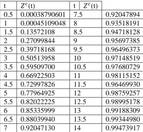
Table 3.Experience 3: α=1, λ=2, Δt=0.01 and Δp=0,001
t (t) t (t) 0.5 0.00038790601 7.5 0.92047894 1 0.00045109048 8 0.93518191 1.5 0.13572108 8.5 0.94718128 2 0.27099844 9 0.95697385 2.5 0.39718168 9.5 0.96496373 3 0.50513958 10 0.97148519 3.5 0.59509700 10.5 0.97680729 4 0.66922503 11 0.98115152 4.5 0.72997826 11.5 0.96469930 5 0.77964925 12 0.98759257 5.5 0.82022225 12.5 0.98995178 6 0.85335999 13 0.99188309 6.5 0.88039940 13.5 0.99344980 7 0.92047130 14 0.99473917
The | | queue busy cycle distribution 87 [ ] [ ] [ ] [ ]
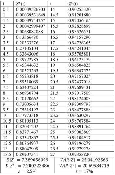
Table 4.Experience 1: α=2, λ=1, Δt=0.01 and Δp=0,01
t (t) t (t) 0.5 0.00039526703 14 0.90255320 1 0.00039531649 14.5 0.91201680 1.5 0.00039744257 15 0.92056465 2 0.00042999497 15.5 0.92828899 2.5 0.0068082088 16 0.93526571 3 0.13566480 16.5 0.94157290 3.5 0.20333376 17 0.94726365 4 0.27105104 17.5 0.95241045 4.5 0.33643096 18 0.95705801 5 0.39722785 18.5 0.96125179 5.5 0.45344632 19 0.96504825 6 0.50523263 19.5 0.96847575 6.5 0.55233818 20 0.97157025 7 0.59518069 20.5 0.97437018 7.5 0.63407224 21 0.97689431 8 0.66930794 21.5 0.97917509 8.5 0.70120662 22 0.98124003 9 0.73005634 22.5 0.98309797 9.5 0.75615197 23 0.98477888 10 0.77973318 23.5 0.98630297 10.5 0.80105113 24 0.98767584 11 0.82031202 24.5 0.98891764 11.5 0.83771467 25 0.99003869 12 0.85343867 25.5 0.99104917 12.5 0.86764937 26 0.99196279 13 0.88047999 26.5 0.99279278 13.5 0.89207541 27 0.99353820 [ ] [ ] [ ] [ ] Received: November 28, 2013