www.nonlin-processes-geophys.net/17/777/2010/ doi:10.5194/npg-17-777-2010
© Author(s) 2010. CC Attribution 3.0 License.
in Geophysics
Simulation of the long-term behaviour of a fault with two asperities
M. Dragoni1and S. Santini2
1Dipartimento di Fisica, Universit`a di Bologna, Viale Carlo Berti Pichat 8, 40127 Bologna, Italy
2Dipartimento di Matematica, Fisica e Informatica, Universit`a di Urbino, Via Santa Chiara 27, 61029 Urbino, Italy
Received: 11 September 2010 – Revised: 22 November 2010 – Accepted: 2 December 2010 – Published: 15 December 2010
Abstract. A system made of two sliding blocks coupled by a spring is employed to simulate the long-term behaviour of a fault with two asperities. An analytical solution is given for the motion of the system in the case of blocks having the same friction. An analysis of the phase space shows that orbits can reach a limit cycle only after entering a particular subset of the space. There is an infinite number of different limit cycles, characterized by the difference between the forces applied to the blocks or, as an alternative, by the recurrence pattern of block motions. These results suggest that the recurrence pattern of seismic events produced by the equivalent fault system is associated with a particular stress distribution which repeats periodically. Admissible stress distributions require a certain degree of inhomogeneity, which depends on the geometry of fault system. Aperiodicity may derive from stress transfers from neighboring faults.
1 Introduction
Spring-block systems are commonly used as low-order analogs of seismic sources. A system made of a block pulled by a spring was first proposed by Burridge and Knopoff (1967). Due to non linear dependence of friction on the block velocity, the system is nonlinear and dissipative.
The simplest friction law that generates the stick-slip behaviour characteristic of seismic sources is a piecewise constant function of slip rate, with friction assuming a static or a dynamic value. More complicated friction laws are obtained from laboratory experiments and have been used in spring-block models (Byerlee, 1978; Dieterich, 1981; Ruina, 1983; Rice and Tse, 1986; Erickson et al., 2008). It has
Correspondence to:S. Santini ([email protected])
been shown that spring-block models can simulate several features of seismic activity (Dieterich, 1972; Rundle and Jackson, 1977; Cohen, 1977; Cao and Aki, 1984, 1986; Gu et al., 1984; Carlson and Langer, 1989a,b; Carlson et al., 1994). The discovery that simple models for seismic sources may exhibit deterministic chaos has raised interest for its implications in earthquake prediction (Keilis-Borok, 1990; Keilis-Borok and Kossobokov, 1990; Beltrami and Mareschal, 1993).
Nussbaum and Ruina (1987) considered a two-block model with spatial symmetry and found periodic behaviour. Huang and Turcotte (1990a, 1992) and McCloskey and Bean (1992) showed that a two-block model without spatial symmetry yields chaotic behaviour. Huang and Turcotte (1990b) showed that the chaotic behaviour may reproduce some features of interacting fault systems. Two-block systems were also considered by de Sousa Vieira (1995) and He (2003).
In the present paper we consider a model made of two coupled blocks, pulled at constant velocity on a rough plane. The model is intended to simulate the behaviour of a fault with two asperities (or of two coplanar fault segments) subject to a constant tectonic strain rate. We assume that the blocks are characterized by the same values of static and dynamic friction.
2 Equations of motion
Consider two blocks having equal mass m and placed on a horizontal plane (Fig. 1a). Each block is connected by a horizontal spring of rigidity K to a driving mechanism moving at constant velocityvin the horizontal direction. The blocks are connected to each other by a spring of rigidityKc. We assume that the motion of each block is resisted by a static frictionfsand a dynamic frictionfd.
We indicate with coordinates x and y the extensions of the springs connecting respectively blocks 1 and 2 to the driver. Following Turcotte (1997), we introduce nondimensional coordinates and time
X=Kx fs
, Y=Ky fs
, T= r
K
mt (1)
We set ǫ=fd fs
, α=Kc
K (2)
with 0< ǫ <1 andα >0. Iff1andf2are the forces applied
to the blocks, we introduce nondimensional forces F1=
f1 fs
, F2= f2 fs
(3) When the blocks are stationary, the equations of motion of the system are then
¨
X=0, Y¨=0 (4)
where dots indicate differentiation with respect toT. When the blocks are moving, the equations are
¨
X+(1+α)X=ǫ+αY (5)
¨
Y+(1+α)Y=ǫ+αX (6)
The system having two degrees of freedom, the phase space is a 4-manifoldS. The evolution of the system is described by the orbit of the representative point inS.
For the largest part of time the system is stationary. Therefore it is natural to assume as initial condition a state withX˙= ˙Y =0. This implies that the representative point belongs to the planeXY. We shall study the projection of the orbit in this plane. In view of the seismological application, we assumeX≥0, Y≥0. SinceXandY vary in the range [0, 1], the projection ofS is the unit square with vertices at (0,0), (1,0), (1,1), (0,1).
3 Solution
In the planeXY the conditions for the motion of block 1 or 2 are represented respectively by the lines
Y=1+α
α X− 1
α (7)
Y= α
1+αX+ 1
1+α (8)
that we name lines 1 and 2, respectively (Fig. 1b). The two lines and the axes X and Y form a quadrilateral Q, with vertices at(0,0),(A,0),(1,1),(0,A)and area
A= 1
1+α (9)
Hence Q is the set of points corresponding to stationary blocks: it coincides with the unit square when α=0, it shrinks progressively as α increases and tends to the diagonalY=Xforα→ ∞. The initial state is then a point P0=(X0,Y0)∈Q.
3.1 Stationary blocks
With initial conditions
X(0)=X0, Y (0)=Y0, X(˙ 0)=0, Y (˙ 0)=0 (10)
Eqs. (4) have the solution
X=X0+V T , Y=Y0+V T (11)
whereV is the nondimensional velocity V=
√
Km fs
v (12)
Eqs. (11) are the parametric equations of the line
Y=X+p (13)
where
p=Y0−X0 (14)
Any segment of line (13) contained inQis a set of states in which both blocks are stationary. Since P0∈Q,pcan vary
within the range [−A,A]. Line (13) will intersect line 1 or 2 depending on the sign ofp.
According to (14), p expresses the difference between the initial displacements of blocks. A more interesting interpretation ofp is based on the forces applied to blocks. From the equations of motion,
F1= −X−α(X−Y ), F2= −Y−α(Y−X) (15)
In the state (X0, Y0) the difference between them can be
written thanks to (14) as
1F=(1+2α)p (16)
acting on the two blocks. If P0is close to the diagonalY=X
(hence|p|is small), the blocks are subject to forces of similar strengths. If P0is far from the diagonal and close to line 1
or 2, one of the blocks is subject to a much greater force than the other. If P0 is in the vicinity of point (1,1), both
blocks are close to the onset conditions and the motion of one of them will easily produce the motion of the other.
Speaking about faults, we can say that the magnitude ofp is a measure of the inhomogeneity of the applied stress. The inhomogeneity has two causes: the difference between the amounts of slip of the two asperities (the termpin (16)) and the effect of coupling (the term 2αp). This means that the stress on the fault is fairly homogeneous when P0is close to
the diagonal, while it is inhomogeneous when P0is close to
line 1 or 2. In the first case the effect of tectonic loading is prevailing, in the second case the effect of a dislocation on the other is important.
3.2 Moving blocks
We solve the equations of motion in the case when only one block slips at a time. The motion of block 1 is given by (5) with initial conditions
X(0)= ¯X, X(˙ 0)=0 (17)
andY equal to a constantY¯ given by (7):
¯
Y=1+α α X¯−
1
α (18)
The solution is X(T )= ¯X−U 2 h
1−cos√1+α Ti (19)
˙
X(T )= −U 2
√
1+αsin√1+α T (20)
where U=21−ǫ
1+α (21)
Equations (19) and (20) are the parametric equations of an ellipse with minor axis U and major axis √1+α U. The block stops at time
T0= π
√
1+α (22)
when the representative point is(X¯−U,Y )¯ . This shows that U is the final displacement of the block. Analogously, the motion of block 2 is given by (6) with initial conditions Y (0)= ¯Y , Y (˙ 0)=0 (23) andXequal to a constantX¯ given by (8):
¯
X=1+α
α Y¯− 1
α (24)
Fig. 1. (a)The two-block system;(b)projection of the phase space in the planeXY and the quadrilateralQ(α=1); (c)noteworthy subsets ofQ: B1, B2, L1, L2, and the set C of limit cycles (ǫ=0.7).
The solution is
Y (T )= ¯Y−U
2 h
1−cos√1+α Ti (25)
˙
Y (T )= −U
2
√
The block stops again at T =T0 when the representative
point is (X¯,Y¯−U). It can be seen that the values ofX˙ andY˙ vary in the range [−1, 0]. HenceSis a hypercube with unit edge. The conditionsX≥0,Y≥0 implyǫ≥1/2.
4 Limit cycles
There are two regions in the phase space from which the orbit of the system enters immediately a limit cycle. They are defined as follows. Let us call L1the subset ofQenclosed
between the lines
Y=X−a, Y=X−b (27)
and L2the subset enclosed between the lines
Y=X+a, Y=X+b (28)
where a= α
1+2αU, b= 1+α
1+2αU (29)
Let P1be the intersection point of line (13) with line 1 or 2
and P2the arrest point of block 1 or 2, respectively. Subsets
L1and L2have the following properties:
1. if P0∈L1, then P1belongs to line 1 and P2∈L2;
2. if P0∈L2, then P1belongs to line 2 and P2∈L1.
The proof is immediate since a displacementUbrings the points belonging to the minor base of the trapezoid L1onto
the major base of the trapezoid L2 and vice versa. Hence,
when the representative point of the system enters the region L = L1∪L2, it remains there forever, jumping an infinite
number of times from L1to L2and vice versa (Fig. 1c).
Consider a point P0∈L1. The orbit of the system in the
planeXY is initially a segment of line (13) which intersects line 1 at P1=(X1,Y1). The orbit is then a segment of line Y=Y1until the arrest point P2=(X2,Y2)of block 1. Then
the orbit is a segment of line
Y=X+p+U (30)
which intersects line 2 at point P3=(X3,Y3). Finally, it is a
segment of lineX=X3 until the arrest point P4=(X4,Y4)
of block 2. It is easy to prove that P4belongs to line (13).
Therefore the system has entered a limit cycle. The same conclusion is reached if P0∈L2. We conclude that:
1. The projectionCpof a limit cycle in the planeXY is the union of four rectilinear segments and has four singular points. Their coordinates are given in Table 1.
2. All points P0∈L with the same value ofpconverge to
the same cycleCp.
3. Points P0∈L1characterized bypconverge to the same
cycle as points P0∈L2characterized byp+U: hence Cp=Cp+U.
Table 1.Coordinates of the singular points of a limit cycle.
(a) P0∈L1
X1=1+αp, Y1=1+(1+α)p X2=1+αp−U, Y2=1+(1+α)p X3=1−(1+α)(p+U ), Y3=1−α(p+U ) X4=1−(1+α)(p+U ), Y4=1−αp−(1+α)U
(b) P0∈L2
X1=1−(1+α)p, Y1=1−αp X2=1−(1+α)p, Y2=1−αp−U X3=1+α(p−U ), Y3=1+(1+α)(p−U ) X4=1+αp−(1+α)U, Y4=1+(1+α)(p−U )
4. There is an infinite noncountable number of cyclesCp withp∈ [−b,−a]. The union of allCpis a setC⊂Q. 5. Each cycle represents the alternate motion of blocks.
If P0∈/L, orbits are in general more complicated: their
projection may be not entirely contained in Qand may be the union of rectilinear and curvilinear segments. Blocks can move simultaneously. It is evident from Fig. 1c that this occurs when P0 belongs to the regions B1 or B2,
corresponding to −a < p <0 and 0< p < a, respectively. In fact, when P0∈B1, the segment describing the motion of
block 1 intercepts line 2 and triggers the motion of block 2. Analogously, when P0∈B2, the motion of block 2 intercepts
line 1 and triggers the motion of block 1. Such orbits reach a limit cycle only when they enter L. We do not consider them in the present paper.
5 Recurrence periods
From the coordinates of singular points, it is easy to calculate the time intervals elapsing between the motions of blocks. We consider the case p <0, including all possible limit cycles. The interval between the motions of block 1 and block 2 is
T12= −
(1+2α)p+αU
V (31)
and that between the motions of blocks 2 and 1 is T21=
(1+2α)p+(1+α)U
V (32)
Aspincreases in the range [−b,−a],T12decreases, while T21increases. The two intervals are equal whenp= −U/2.
If we neglect the duration of block motions, the interval elapsing between two consecutive motions of the same block is
1T=T12+T21= U
which is independent ofpand therefore is the same for all cycles. If we define
r=T12 T21
(34) we can write
p= − (1+α)r+α
(1+2α)(1+r)U (35)
This shows that a limit cycle can be characterized by r instead ofp. Thanks to (16) and (35), the difference between forces when the system enters a limit cycle is
1F= −(1+α)r+α
1+r U (36)
This pattern repeats periodically in the cycle and character-izes it. The intensities of forces at singular points are given in Table 2.
In conclusion, in any limit cycle the recurrence period1T of motions of each block is the same for both blocks, for given values ofǫandα. However the periodsT12 andT21
elapsing between the motion of one block and that of the other depend on the shape of the cycle, which in turn depends on the distribution of forces on the blocks.
If we suppose that the displacement of a block corresponds to the slip of a fault asperity, we can calculate the seismic moment releaseM(T )as a function of time. Assume that asperity 1 fails atT =0 and the moment release associated with the slip of each asperity isM0. The cumulative release
is then
M(T )=M0 N X
n=0
[H (T−n1T )+H (T−T12−n1T )] (37)
whereH (T )is the Heaviside function andNis a very large integer. In the particular caseT12=0, (37) reduces to
M(T )=2M0 N X
n=0
H (T−n1T ) (38)
representing a sequence of events with period 1T and seismic moment 2M0. In the caseT12=1T /2, (37) can be
written as
M(T )=M0 N X
n=0 h
HT−2n1T 2
+HT−(2n+1)1T 2
i
(39) which reduces to
M(T )=M0 2N X
m=0
HT−m1T 2
(40)
representing a sequence of events with period 1T /2 and momentM0.
Table 2. Intensity of forcesF1andF2at the singular points of a
limit cycle.
Point F1 F2
P1 −1 −1−(1+2α)p
P2 −1+(1+α)U −1−(1+α)p−α(p+U )
P3 −1+(1+2α)(p+U ) −1
P4 −1+αp+(1+α)(p+U ) −1+(1+α)U
6 Discussion and conclusions
Fault surfaces are characterized by an inhomogeneous distribution of friction. Such a distribution is commonly represented in the framework of an asperity model, which distinguishes between high- and low-friction patches on the fault (Lay et al., 1982). In addition, friction is governed by a constitutive equation implying that friction may change with time during fault slip and even when the fault is at rest.
We simplify this picture by considering a system having a finite number of degrees of freedom, which includes the essential properties of real faults but avoids the many complications associated with them. This allows us to follow the evolution of the system in the phase space and to investigate its dynamical properties in the long term.
The system of two coupled blocks includes the essential features of a fault with two asperities. Huang and Turcotte (1990a) studied the case in which the blocks have different frictions and found that the system exhibits chaotic behaviour for certain values of the coupling constantα.
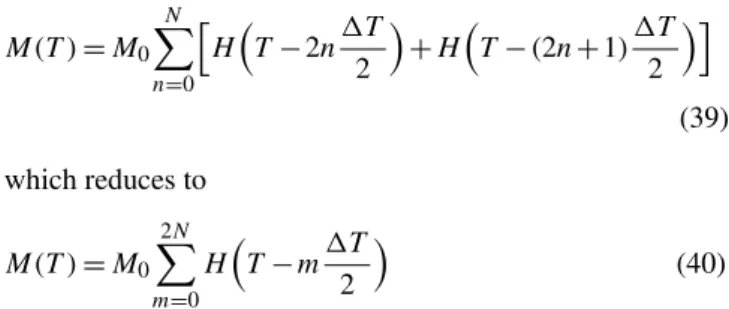
The analysis of the symmetric model presented in this paper shows that the system exhibits a rich phenomenology even in this simpler case. The evolution of the system depends on a parameter p indicating the degree of inhomogeneity of the applied stress. Only a limited range of stress distributions allows the system to enter a limit cycle. In this case the behaviour is periodic, with the alternate motion of the two blocks, but an infinite variety of cases is possible. Figure 2 shows three different limit cycles, corresponding tor=1, 1/5 and 0. Cases withr >1 yield similar cycles with the roles of the two blocks interchanged. If we set α=1, it follows A=1/2, a=U/3 and b=2U/3. The cycles correspond top/U= −1/2, −7/18 and−1/3. We take ǫ=0.7 (Scholz, 1990), implying U=0.3. Figure 3 shows the seismic moment releaseMand the forcesF1,F2
as functions of time for the three cases.
Fig. 2.Three possible limit cycles of the system, for different values of the ratior(α=1,ǫ=0.7).
Fig. 3. Seismic moment releaseMand forcesF1,F2as functions
of time for the cycles shown in Fig. 2.
in time, followed by a long interseismic period, equal to 1T /(r+1)orr1T /(r+1), respectively. The case in which one of the intervals is close to 0 corresponds to a fault where the failure of an asperity is followed immediately by that of the other, producing a single earthquake with moment 2M0
Due to the dependence on p, the shape of limit cycles depends on the stress distribution. The condition under which fault slips are close in time takes place for relatively small and relatively large values of|p|, while fault slips are equally spaced in time when |p| assumes an intermediate value. Hence the recurrence pattern of seismic events depends on the stress distribution in the system. A certain distribution of seismic events in time corresponds to a stress distribution that repeats periodically: it is the stress distribution that was present when the system entered the limit cycle.
A critical parameter of the system is the coupling constant α. In order to evaluate which values are appropriate for it, we compare the spring-block model with a simple model based on continuum mechanics. We consider a vertical, plane fault embedded in a shear zone of widthd and rigidity µ, subject to a constant strain rate (Dragoni and Tallarico, 1992). Two coplanar asperities having the same areaAare placed at distanceR on the fault. In the point-like source approximation, the shear stress transferred to one asperity by slip1uof the other asperity can be written as
σ≈µ1uA
R3 (41)
A comparison between the two models yields the correspon-dence rules
Kc≈ µA2
R3 , K≈µd (42)
whence α≈ A
2
R3d (43)
showing thatαis related to the geometry of the fault system. The valueα=1 adopted in the graphs corresponds toA=
107m2,R=104m,d=102m.
As coupling increases, the areaAof Qdecreases, hence the set of states where both blocks are stationary is reduced. It is easy to see that the area of L reduces more rapidly than A. Hence, whenαis large, the initial state of the system is more likely to be outside L, with the consequence that the system will not enter immediately a limit cycle. At the same time, an increasing coupling makes stress less homogeneous according to (16) and the stress transferred from one asperity to the other during a cycle greater. On the contrary, tectonic stress is prevailing whenαis very small.
Observation shows that the seismogenic activity of a fault is aperiodic and generates earthquakes of different magnitudes. This behaviour can easily result from the present model if we assume that the system is not isolated. It is sufficient that stress is transferred to the system from neighboring faults (in connection with earthquakes produced by them) in order that the system moves each time from one limit cycle to another having a different recurrence pattern. In the block model, a small force perturbation on the blocks
may change the value ofpaccording to (16), thus addressing the representative point to a different limit cycle with a different value ofr: this is expressed by the derivativedr/dp. In a fault system, the recurrence times of earthquakes generated by a specific fault in the periodic, limit-cycle regime are easily longer than the recurrence times of perturbations by neighboring faults. If the fault model considered here is subject to such perturbations, the fault will enter a limit cycle, but will not remain long in it due to intervening stress perturbations. Therefore periodicity could not be observed in most cases.
Acknowledgements. We thank the editor L. Telesca and two anonymous referees for useful comments and suggestions on the paper.
Edited by: L. Telesca
Reviewed by: two anonymous referees
References
Beltrami, H. and Mareschal, J.-C.: Strange seismic attractor?, Pure Appl. Geophys., 141, 71–81, 1993.
Burridge, R. and Knopoff, L.: Model and theoretical seismology, B. Seismol. Soc. Am., 57, 341–371, 1967.
Byerlee, J.: Friction of rocks, Pure Appl. Geophys., 116, 616–626, 1978.
Cao, T. and Aki, K.: Seismicity simulation with a mass-spring model and a displacement hardening-softening friction law, Pure Appl. Geophys., 122, 10–23, 1984.
Cao, T. and Aki, K.: Seismicity simulation with a rate and state dependent friction law, Pure Appl. Geophys., 124, 487–513, 1986.
Carlson, J. and Langer, J.: Mechanical model of an earthquake fault, Phys. Rev. A, 40(11), 6470–6484, 1989a.
Carlson, J. and Langer, J.: Properties of earthquakes generated by fault dynamics, Phys. Rev. Lett., 62(22), 2632–2635, 1989b. Carlson, J., Langer, J., and Shaw, B.: Dynamics of earthquake fault,
Rev. Mod. Phys., 66(2), 657–659, 1994.
Cohen, S.: Computer simulation of earthquakes, J. Geophys. Res., 82, 3781–3796, 1977.
de Sousa Vieira, M.: Chaos in a simple spring-block system, Phys. Lett. A, 198, 407–414, 1995.
Dieterich, J. H.: Time dependent friction as a possible mechanism for aftershocks, J. Geophys. Res., 77, 3771–3781, 1972. Dieterich, J. H.: Constitutive properties of faults with simulated
gouge, in: Mechanical Behavior of Crustal Rocks, edited by: Carter, N. L., Friedman, M., Logan, J. M., and Stearns, D. W., Am. Geophys. Union, Geophys. Monogr., 24, 103–120, 1981. Dragoni, M. and Tallarico, A.: Interaction between seismic and
aseismic slip along a transcurrent plate boundary: a model for seismic sequences, Phys. Earth Planet. In., 72, 49–57, 1992. Erickson, B., Birnir, B., and Lavall´ee, D.: A model for
Gu, J. C., Rice, J. R., Ruina, A. L., and Tse, S. T.: Slip motion and stability of a single degree of freedom elastic system with rate and state dependent friction, J. Mech. Phys. Solids, 32, 167–196, 1984.
He, C.: Interaction between two sliders in a system with rate- and state-dependent friction, Science in China, Series D, 46, 67–74, 2003.
Huang, J. and Turcotte, D. L.: Are earthquakes an example of deterministic chaos?, Geophys. Res. Lett., 17, 223–226, 1990a. Huang, J. and Turcotte, D. L.: Evidence for chaotic fault
interactions in the seismicity of the San Andreas fault and Nankai trough, Nature, 348, 234–236, 1990b.
Huang, J. and Turcotte, D. L.: Chaotic seismic faulting with mass-spring model and velocity-weakening friction, Pure Appl. Geophys., 138, 569–589, 1992.
Keilis-Borok, V. I.: The lithosphere of the Earth as a nonlinear system with implications for earthquake prediction, Rev. Geophys., 28, 19–34, 1990.
Keilis-Borok, V. I. and Kossobokov, V. G.: Premonitory activation of earthquake flow: algorithm M8, Phys. Earth Planet. In., 61, 73–83, 1990.
Lay, T., Kanamori, H., and Ruff, L.: The asperity model and the nature of large subduction zone earthquakes, Earthquake Pred. Res., 1, 3–71, 1982.
McCloskey, J. and Bean, C. J.: Time and magnitude predictions in shocks due to chaotic fault interactions, Geophys. Res. Lett., 19, 119–122, 1992.
Nussbaum, J. and Ruina, A.: A two degree-of-freedom earthquake model with static/dynamic friction, Pure Appl. Geophys., 125, 629–656, 1987.
Rice, J. R. and Tse, S. T.: Dynamic motion of a single degree of freedom system following a rate and state dependent friction law, J. Geophys. Res., 91, 521–530, 1986.
Ruina, A.: Slip instability and state variable friction laws, J. Geophys. Res., 88, 10359–10370, 1983.
Rundle, J. B. and Jackson, D. D.: Numerical simulation of earthquake sequences, B. Seismol. Soc. Am., 67, 1363–1377, 1977.
Scholz, C. H.: The Mechanics of Earthquakes and Faulting, Cambridge University Press, Cambridge, 1990.