Economic growth and equity returns : application to the chinese stock market

(1)

M

ONETARY AND

M

ASTER

ECONOMIC GROWTH AND

APPLICATION TO THE CHIN

Y

ULIN

A

N

S

UPERVISION

:

A

NTÓNIO

A

FONSO

ONETARY AND

F

INANCIAL

E

CONOMICS

ASTER

´

S

F

INAL

W

ORK

D

ISSERTATION

ECONOMIC GROWTH AND EQUITY RETURNS:

LICATION TO THE CHINESE STOCK MARKET

D

ECEMBER

2018

CONOMICS

EQUITY RETURNS:

ESE STOCK MARKET

(2)

(3)

3

This dissertation provides new insights on the estimation of the long run expected equity return in China, following the framework of Cornell (2010) on Economic Growth and Equity return, taking into consideration of convergence in economic growth, thus extending the research scope from mature countries to emerging market. We assess the period 1990-2017, explore the long run expected equity return in China, and we find that it should not be more than -0.5% over the long run.

JEL Codes: O4; E2; G1; M4.

(5)

5

1. Introduction

In this thesis we estimate the long run expected equity return in China. Regarding the significance of the long run expected equity return, this differs for different market players. For example, for equity investors, it is the long run return they could profit from; for fund managers, it is a benchmark to assess their long run performance; for a policy-maker, it is an indicator on macroeconomic conditions. Because the equity return is very sensitive, many countries treat it as barometer of macroeconomic conditions. Since the stock market could reflect the macroeconomic conditions, we could reasonable think macroeconomic conditions, largely, determine stock. In short, economic growth caps equity earnings growth.

From a theoretical perspective, we follow Cornell’s (2010) analysis on economic growth and Equity returns taking into consideration economic growth convergence, and extend the research scope from mature countries to emerging markets. Empirically, we apply the methodology to the largest emerging countries i.e. China. Specifically, we collect the relevant data from year 1990 to year 2017, and explore the long run expected equity return in China, which should not be more than -0.5%.

The remainder of the thesis is organised as follows. Section 2 provides the literature. Section 3 illustrates the methodology on estimating growth rate of equity market value. Section 4 reports the empirical analysis. Section 5 is the conclusion.

2. Literature

Cornell (2010) shows that the performance of equity investment is linked to economic growth. Theoretically, he bridges the gap between economic growth and earnings growth. Empirically, he observes that real GDP per capita growth and population growth contribute to earnings growth, validates the fact that earnings-to-GDP ratio is stationary, finds the net dilution effect and dividend yield in the case of the S&P 500 index. He reaches the conclusion that over the long run,

(6)

6

investors should anticipate real returns on common stock to average no more than 4 percentage in the U.S.

Arnott and Bernstein (2002) gauge the risk premium for stocks relative to bonds. Therefore, they gauge bond yields, expected real stock returns, stock dividend yields and real dividend growth. They demonstrate that the long-term forward-looking risk premium is not near the level of the past, in 2002, and that the risk premium may well be near zero, perhaps even negative in the U.S.

Fama and French (2002), estimate the equity premium using dividend and earnings growth rates to measure the expected rate of capital gain from 1951 to 2000. The results they obtain, 2.55% and 4.32%, are much lower than the equity premium produced by the average stock return. Their evidences suggest that the high average return for 1951 to 2000 is due to a decline in discount rates that produces a large unexpected capital gain. In other words, the high return for 1951 to 2000 seems to be the result of low expected future returns in the U.S..

3. Methodology on Estimating the Growth Rate of Equity Market Value

Obviously, the performance of equity investment has connections with economic growth. Indeed, in a robust and sustainable growth environment, public companies, usually the dominant entities in the economy will enjoy decent earnings. Hence, healthy earnings could bring enough free cash flow, thus increase the market value of the listed companies. The enhancement in the market value of listed companies would be reflected on the stock price in the secondary market and increase dividend payment. As a result, the performance of equity returns would be improved. Intuitively, the relation between economic growth and equity returns is positive. Furthermore, it is understandable that it is economic growth that determines equity return rather than the other way around. Therefore, long-run earnings’ returns are restricted by economic growth.

Theoretically, we could explore the mathematical relation between equity return and economic growth from a quite simple equation that would ever hold:

(7)

7

(1) P=P,

where P is the market value of entire equity market.

In order to bridge the gap between long-term equity return and economic growth, we could introduce output into equation, therefore we could make the following transformation:

(2) P= × ×Y,

where the variables in equation 错误！未找到引用源。 are: E represents the earnings of

all public companies in the equity market, and Y is the output. Noticeably, both (P/E) and (E/Y) are very important financial indicators in the finance. (P/E) stands for the price to earnings ratio, the most popular valuation indicator in practice. Maybe the expression of (E/Y) is less obvious, but if we replace Y with aggregate revenue for all the public companies in the stock market, (E/Y) becomes the most significant profitability indicator in finance, i.e. the net profit margin. Since in the thesis, we always discuss the performance of the public companies in the stock market. we always treat (E/Y) as net profit margin.

To analyse the relationship between equity prices, price-to-earnings ratio, net profit margin and output, we can take logs of equation (2):

(3) ln(P)=ln(P

E)+ln( E

Y)+ ln(Y).

Afterwards, we differentiate both sides of the equation, and obtain a new equation revealing the economic intuition between all the economic variables:

(4) = + ( / )

/ +

( / )

/ .

The economic intuition of (4) is that the growth rate of equity market value is equal to the growth rate of output plus the growth rate of net profit margin, plus the growth rate of the P/E ratio. Later we will show that both net profit margin and price-earnings ratio are stationary. Thus, it is reasonable to assume that the net profit margin growth rate and the P/E ratio growth rate are zero. Therefore, in the long run,

(8)

8

the growth rate of equity market value is dominated by the growth rate of output. Therefore, we could simplify (4) as follows:

(5) = .

As we know, economic, political, and even social factors could have an impact on the equity market, and this is the reason why it is difficult to assess equity performance in practice. However, equation (5) hints at an alternative method to focus on the output growth in the long-run.

When we refer to output growth, it is possible to find a framework in the economic growth theory. The Solow growth model is the benchmark model in economic growth theory, and the most significant insight of Solow’s growth model, as referred by Romer (2012), is that no matter what is the economic condition, the economy will eventually converge to a balanced growth path. On the balanced growth path, the growth rate of output per capita, usually seen as a living standard, is solely determined by the technological progress growth rate.

Solow (1956) shows that in the context of a balanced growth path, per capita capital does not change. Formally, the change in per capita capital is the difference between actual investment and breakeven investment. Actual investment is the product of the savings rate and the production function, and the breakeven investment is a linear function of per capita capital. Because of the assumption that Inada condition holds, the production function is concave, so the actual investment is concave. By contrast, the breakeven investment is linear, so it is not difficult to understand the two curves must eventually cross at one point apart from the origin. Initially, when per capita capital is smaller than the steady state level of capital, actual investment is larger than the breakeven investment, the change in per capita capital is positive so capital per capita is rising. By contrast, when per capita capital is larger than the steady state capital per capita, breakeven investment is larger than actual investment, the change in capital per capita is negative so capital per capita is decreasing. Eventually, when capital per capita equals the steady state capital per capita, the change in capital per capita is zero, per capita capital will remain constant.

(9)

9

From an economic perspective, because the production function satisfies the Inada condition, these conditions (which are stronger than needed for the model’s central results) state that the marginal product of capital is very large when the capital stock is sufficiently small and that it becomes very small as the capital stock becomes large. Consequently, rational producers stop adding capital when the marginal product of capital drops to its marginal cost. When the economy reaches that point, it is said to be in a steady state. Once the economy reaches the steady state growth path, the ratio of capital per capita remains constant and output per capita growth ceases. Therefore, we could use Equation (6) to describe the conclusion of the Solow growth model: (6) ( )

/ = g.

where g is the technology growth rate, and Y/L is output per capita. Combining equation (5) and (6), we can write equation (7): (7) = = g + n.

where n is the population growth rate, which accounts for the labour growth rate. In the Solow growth model, on the balanced growth path, the growth rate of output is the sum of technology growth rate and population growth rate. Therefore, the growth rate of the equity market value is determined by the technology growth rate and the population growth rate.

Therefore, to estimate the growth rate of equity market value we need to: - Estimate the technology growth rate and population growth rate;

- Prove that the net profit margin (E/Y) and price earnings ratio (P/E) is stationary over the long term.

It is also noticeable that only when the economy is in the steady state that the per capita output growth is exclusively determined by technological progress growth. Otherwise, we must consider convergence, i.e. the so-called “catch-up effect”. If the per capita capital is still less than the steady state required capital per capita, then the marginal product of capital is still larger than the marginal cost of capital. In this situation, if more capital per capita are invested, output per capita will increase.

(10)

10

Therefore, output per capita growth will exceed the technology growth due to “capital-deepening effect”. In other words, we should consider convergence when the observed economy is an emerging country such like China.

4. Empirical analysis

4.1. Technological Progress and Population Growth

Barro and Ursua (2008) considered a dataset on world economic growth from 1923 to 2006. Country group A includes mature economies such as, for instance, the United States, the United Kingdom, Germany, and Japan. Considering the share scale of market value of China is limited, until 2006, country group A almost accounts for the entire global market capitalization. Real growth rates of per capita GDP are obviously homogenous with a merely standard deviation of 0.42. The average real growth rate in per capita GDP is 2.19%. Notably, the real growth rate in per capita GDP of United States is only 1.14%. Obviously, the most representative sample in group A is the United States, notably because of the dominant weight of the United States equity market. Hence, it is the country that is most approaching to the steady state. Therefore, it is reasonable to use no more than 2% to estimate real growth rate in per capita GDP for mature markets, i.e. the growth rate of technology g.

By contrast, the developing countries are more heterogeneous with a standard deviation as far as 0.75. The emerging markets show rapid convergence because of the capital-deepening effect. The average real growth rate in per capita GDP for emerging markets is 2.32% in the corresponding period.

(11)

11

Table 1. Real Growth Rate in per Capita GDP and Annual Population Growth Rate in China

Year GDP per capita growth rate（%） Annual Population Growth Rate（%） 1990 2.39 1.47 1991 7.81 1.23 1992 12.82 1.15 1993 12.57 1.15 1994 11.78 1.13 1995 9.75 1.09 1996 8.78 1.05 1997 8.12 1.02 1998 6.81 0.96 1999 6.74 0.87 2000 7.64 0.79 2001 7.56 0.73 2002 8.40 0.67 2003 9.35 0.62 2004 9.46 0.59 2005 10.74 0.59 2006 12.09 0.56 2007 13.64 0.52 2008 9.09 0.51 2009 8.86 0.50 2010 10.10 0.48 2011 9.01 0.48 2012 7.33 0.49 2013 7.23 0.49 2014 6.76 0.51 2015 6.36 0.51 2016 6.12 0.54 2017 6.30 0.56 Source: https://data.worldbank.org.

Specifically, in the case of China, in the last 30 years we have witnessed significant economic development. For instance, Wu (2016) illustrated several reasons for such economic growth: first, economic reform encouraged

(12)

12

entrepreneurship and start-ups; second, entrepreneurship transfers inactive economic factors such as labour and land to most economic efficient sectors, so that the total factor productive rate is enhanced; third, taking advantage of lower saving rates and shortage of investment in advanced countries, China’s opening-up policy enabled itself to export more products to other countries to eliminate the negative impact from the shortage of internal demand; fourth, the opening-up policy meanwhile led to imports of advanced equipment and technology, bridging the gap between advanced countries and China in technology applications.

We collected data for the real growth rate of per capita GDP of China from World Bank database. Table 1 shows the real growth rate in per capita GDP and annual population growth rate for China from 1990 to 2017 corresponding to the history of the Shangai Stock Exchange (SSE) composite index.

Considering that the geometrical mean has advantages compared to arithmetical mean when calculating the annual compounding growth rate, we computed the geometrical mean on the real growth rate of per capita GDP for China during the 27 years under analysis, which is 8.67%. Compared to the findings of Barro and Ursua (2008) that Taiwan had the highest real growth rates in per capita GDP as high as 3.78% from 1923 to 2006, China’s growth rate was then higher.

In fact, China has started to develop since the government implemented economic reforms and an opening-up policy in the 1980s. Initially, it is a less developed country who was far from the steady state. With the implementation of the abovementioned policy, a large scale of foreign capitals rushed into China, helping the process of “capital-deepening” in a relatively short time. During this process, the catching up effect of convergence played a significant role, thus China achieved very high economic growth rates. When we observe the recent 8 years regarding real GDP per capita growth rate, it is not difficult to find it declines gradually, which supports the conclusion on convergence speed of Romer (2012): such convergence speed has a positive relation with the distance between actual per capita capital and steady state capital per capita.

(13)

13

Therefore, what we should emphasis is that the 8.67% growth rate includes both technology progress and a convergence effect. Hence, we could not expect more than 9% real growth rate in per capita GDP in China to estimate the technology progress and the convergence effect.

As it is shown in equation (7), when we consider the growth rate of total output, we should not only consider the technology growth rate, but also the population growth rate. The Solow growth model takes population into account, and assumes the population growth rate, n, as an exogenous parameter. Hence, we should consider the effect of population growth when we convert the growth of the per capita output to total output growth.

In practice, instead of the output per capita, the revenue of public listed companies relies on total output. For example, we could assume an economy without any technology progress. If all the conditions hold except that population doubles, in order to satisfy the demand of an increased population, firms should double their products and services. Accordingly, the corporate revenue will double. However, for a mature corporate and industry, the net profit margin usually does not fluctuate significantly and later we will show it is stationary over the long term. Therefore, earnings will double, which will double the returns from the stock prices. Therefore, it is necessary to estimate the population growth rate.

The U.S. Central Intelligence Agency’s 2008 World Fact Book presents the historical population growth rate from 2000 to 2007 for both developed economies (Group A) and emerging market economies (Group B). The average growth rates for those two groups are 0.34% and 0.94% respectively. Moreover, the difference between historical data and projected data is very small, showing the slowly changing nature of population growth rate.

(14)

14

Source: https://data.worldbank.org.

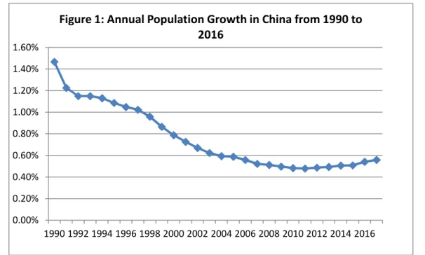
Similarly, we also collected the data on annual population growth rate from the World Bank database. Table 1 shows the annual population growth rate of China from 1990 to 2017 corresponding to the history of SSE composite index. As illustrated in Figure 1, during these 27 years, the annual population growth rate plunged significantly from 1.47% to 0.56%. There are several reasons why China’s population growth rate has such a huge drop. Firstly, and most importantly, China has carried on the one-Child policy from the 1980s, and after the initial resistance from citizens, they started following that policy from 1990s onwards. Secondly, as referred by Weil (2009) population growth is negatively correlated with per capita GDP.

With an 8.67% annual compounding real growth rate in per capita GDP in China during in the past 27 years, the development of the economy was very rapid. In addition, the process of urbanization also played a very important role in the decrease of population growth, since normally, population growth rates are higher in the rural regions compared to the urban region. Until 2011, the population in the urban regions was 51.27% of total population in China, exceeding the population in the rural areas. Thirdly, social and cultural structure experiences changed due to society-opening, for instance, dual income no kids (Dink) families and core families are becoming popular, which are not accepted by the traditional culture of China. Lastly and interestingly,

0.00% 0.20% 0.40% 0.60% 0.80% 1.00% 1.20% 1.40% 1.60% 1990 1992 1994 1996 1998 2000 2002 2004 2006 2008 2010 2012 2014 2016

Figure 1: Annual Population Growth in China from 1990 to 2016

(15)

15

since the 1990s, the Chinese universities started to expand enrolment of university students, and the enrolment rate increased from 34% in 1998 to 75% in 2012. More female university students will increase the employment rate of female, postpone the marriage and thus decrease the population growth.

Since we have computed a geometrical mean of annual compounding population growth rate is 0.79%, if this trend continues, the population growth rate is less likely to recover to 1% in the future. Thus, we could conclude that population growth will not contribute more than 1% to output growth. Given the 9% real growth rate in per capita GDP, this assumption implies that investors cannot reasonably expect long-run future growth in total real GDP to exceed 10%.

4.2 The Stationarity of Net Profit Margin and of the P/E ratio

The net profit margin is equal to net income divided by total revenue, and represents how much profit each dollar of sales generates. From the time series data on the company’s net profit margin, we could assess whether current business practices benefit the company's performance. From the cross section data on the company’s net profit margin, we could judge the competitiveness and profitability of this company in the industry.

From the view of equity valuation, it is also necessary to distinguish earnings from revenue. When one estimates the value of equity, instead of revenue, it is to earnings that one applies the discounted-cash-flow model. As we mentioned before, mathematically, going from equation (4) to equation (5), we assume that ( / )

/ =0, i.e.

the net profit margin growth, for the society as a whole, is 0 over the long term. Only under this assumption, our conclusion holds. Therefore, we should certify that the earnings to GDP ratio (E/Y) is always stationary.

Cornell (2010) has shown that aggregate earnings are a stationary fraction of GDP in the U.S. in the period 1947-2008, and there is no persistent decrease or increase for the earnings-to-GDP ratio. Thus, the earnings growth rate and total output

(16)

16

growth rate are similar in the long run. Mathematically, this earnings-to-GDP ratio is stationary, over the long term, and it is reasonable to assume ( / )

/ =0.

To be more specific, he used two primary measures of aggregate earnings in the United States. One measure of aggregate earning is derived from the national income and product accounts (NIPAs), in which the aggregate cooperate earning is the profits collected from corporate income tax returns. The other measure of aggregate earnings is derived from S&P data collected from corporate financial reports. There are some differences between the two measures. From an accounting perspective, NIPAs is more cash basis, and corporate earnings only include current cash inflow of production less current cash outflow of expenses. Compared to the earnings of NIPAs, S&P data is more accrual basis. Based on the principle of matching, management could tailor the financial reports to reveal more relevant and reasonable information to their investors. Despite these difference, Cornell (2010) finds that regardless of which measure is chosen, no evidence exists of a persistent decrease or increase for the earning to GDP ratio. In practice, he not only observed that data could support the hypothesis that E/GDP is stationary, but also found that earnings growth reflected mean reversion. The net profit margin was not constant, varying between 3 percentage and 11 percentage. In addition, when earnings are low relative to GDP, they grow more quickly, the reverse is true when earnings are relatively high. Therefore, the mean reversion in the growth rate of earnings could also support the stationary of net profit margin.

Because of the data unavailability in China and a short history of the of SSE index, we collected data on earnings and revenues for all the public companies from 1999 to 2017. All the data are downloaded from database WIND that is the most reputable and reliable database in China. During this 19-year period, the number of public companies increased 115%, from 669 to 1442. In that period total earnings increased from 54,603 million Yuan to 2,882,156 million Yuan, with an annual compounding growth rate of 24.65%. The only decrease occurred during the global recession in 2008, with a 11.31% drop. Correspondingly, the total revenues increased

(17)

17

from 787,925 million Yuan to 29,720,010 million Yuan, with a similarly annual compounding growth rate of 22.35%. It is noticeable that the total revenue has never experienced any decrease in that period (see Figure 2 and Figure 3).

Source: WIND database.

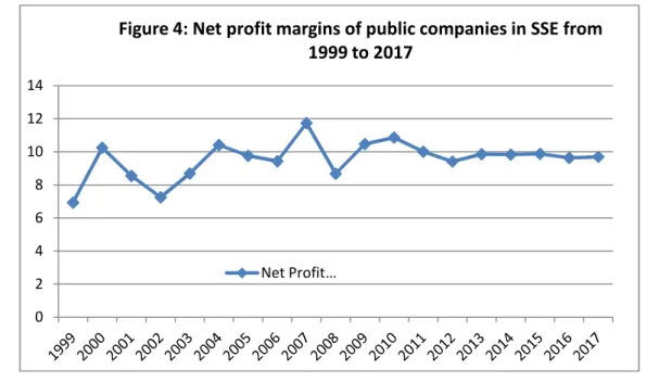
We obtain the net profit margin by dividing the earnings by revenues for each year, and we can observe the net profit margin is stationary. The net profit margin in year 1999 was 6.93%, while it was 9.69% in the year 2017. The maximum data is 11.73%, the minimum data is 6.93%, and the standard deviation is 1.51. From the Figure 4, we could also observe that net profit margin does not show any trend during the 19 years, fluctuating around the geometric mean 9.47%.

-500,000.00 1,000,000.00 1,500,000.00 2,000,000.00 2,500,000.00 3,000,000.00 3,500,000.00 19 99 20 00 20 01 20 02 20 03 20 04 20 05 20 06 20 07 20 08 20 09 20 10 20 11 20 12 20 13 20 14 20 15 20 16 20 17

Figure 2: Earnings of public companies in SSE from 1999 to 2017

Earning -5,000,000.00 10,000,000.00 15,000,000.00 20,000,000.00 25,000,000.00 30,000,000.00 35,000,000.00 19 99 20 00 20 01 20 02 20 03 20 04 20 05 20 06 20 07 20 08 20 09 20 10 20 11 20 12 20 13 20 14 20 15 20 16 20 17

Figure 3: Earnings of public companies in SSE from 1999 to 2017

(18)

18

As referred by Dongwei and Yangru (2005), they took a sample of 467 public companies in SSE, used their fundamental information to calculate financial indicators to reflect profitability, operational capacity, solvency, liquidity and sustainable growth rate. They did the panel data unit root test. They calculated three statistics, which were the Levin-Lin-Chu statistic, the Im-Peraran-Shin t statistic, and the Im-Peraran-Shin LM statistic. They rejected the null hypothesis that sample data have a unit root, and accepted the alternative hypothesis that sample data are stationary. To be more specific, the test result showed that the net profit margin was significantly stationary at 1% level for all three statistics.

Therefore, the data from the SSE index could meet the request that E/GDP is stationary over the long-run. Thus, we could only expect the earnings growth rate match but not exceed the GDP growth rate. By the discounted-cash-flow model, we could not expect the equity return to be more than GDP growth rate. As we discussed at the beginning of the paper, GDP growth rate caps the earnings return.

The price-to-earnings ratio (P/E) is a widely used valuation indicator in the investment industry. When evaluating the intrinsic value of the shares, the P/E is very important regardless of the type of the market (mature or emerging). In the same market and same industry, different public companies with the similar fundamental information should have similar price to earnings multiples, otherwise, there would be

0 2 4 6 8 10 12 14

Figure 4: Net profit margins of public companies in SSE from 1999 to 2017

(19)

19

arbitrage opportunities, i.e. if one listed company A has the same fundamental information as another listed company B.

We can provide an example assuming firm A and firm B have the same earnings amounting to 1 dollar. Both of them are in the same industry and stock market, however, the P/E ratio of company A is 20 but the P/E ratio of company B is only 15, we could reach a conclusion that the share price of A is overestimated or the share price of B is underestimated. This is the so-called “law of one price”. If it does not hold, theoretically, investors would arbitrage by taking advantage of it. In the above example, investors could borrow one share of company A and sell it immediately, obtaining 20 dollars. Then he could buy one share of company B with 15 dollars, remaining 5-dollar profit. With more and more investors taking arbitrage, the share price of company A will decrease and the share price of company B will increase, most importantly, both of share A and share B would have the same price eventually because both of the companies have the same fundamental information. In the end, the investor could sell the share B in his hand to and buy share A with the cash, and return share A. Therefore, this investor profit 5 dollar without any cost. As referred to by Nicholson (1960), covering data for the past years, would indicate a contrary conclusion i.e. that on average the purchase of stocks with low price-earnings multiples will result in a greater appreciation in addition to the higher income provided.

Campbell and Shiller (1998) used the long run annual U.S. dataset on the S&P 500 index from 1872 to 1990, finding that the price-to-earnings ratio had normally moved in a range from 8 to about 20, with a mean of 14.2, and occasionally spiked down as far as 6 or up as high as 26. Moreover, the P/E ratio did not show any trend and is mean reverting. More importantly, the past century had witnessed the fundamental transformation on the U.S. economy, e.g. the predominant economic sector changed from agriculture to industry and then to services. In addition, information technology changed the transport and communication, massive production was replaced by smaller but more flexible organization, however,

(20)

20

empirical research showed that price-earnings ratios fluctuated within in a fairly well-defined range, without strong trends or sudden breaks. From the findings of Campbell and Shiller, our assumption that price-earnings ratio is stationary holds quite well.

Because of the short history and data unavailability of the SSE, we collected the monthly P/E ratio of SSE index from Jan, 1999 to Dec 2017. In these 228 observations, the maximum is 69.64, the minimum is 9.76, the mean is 27.19, and most importantly, the standard deviation is as high as 14.54. We could find the fluctuations of the P/E ratio in Figure 5.

Source: SHANGHAI STOCK EXCHANGE STATISTICS ANNUAL 2005-2017

From the performance of the P/E ratio, we could observe that as an emerging market, the SSE market shows some worth noticing features. First, the fluctuation is very substantial. Parts of the fluctuations could be explained by the distribution of the investors. Compared to a mature financial market such as U.S., instead of institutional investors, it is individual investors that dominate the SSE market. The SHANGHAI STOCK EXCHANGE STATISTIC ANNUAL (2018) shows, that until the end of 2017, there were 48.6 thousand institutional investors while there were 39,343.1 thousand individual investors, almost accounting for 99.78% of the market. In addition, individual investors hold market value of shares amounting to 5.9 trillion

0 10 20 30 40 50 60 70 80 Ja n-99 N ov -9 9 Se p-00 Ju l-0 1 M ay -0 2 M ar -0 3 Ja n-04 N ov -0 4 Se p-05 Ju l-0 6 M ay -0 7 M ar -0 8 Ja n-09 N ov -0 9 Se p-10 Ju l-1 1 M ay -1 2 M ar -1 3 Ja n-14 N ov -1 4 Se p-15 Ju l-1 6 M ay -1 7

Figure 5: Price to earning ratio in SSE from 1999 to 2017

(21)

21

accounted for 21.17% while the institutional investors merely hold market value of shares amounting to 4.52 trillion, accounting for 16.63%.

In terms of the individual investors’ behaviour, they would buy shares when they price goes up and sell them when price drop down, especially when there are market panics or market bubbles, their performance can be less rational than institutional investors. All these preferences lead the fluctuations to become more dramatic. Moreover, compared to the mean of P/E ratio of 14.2 in the U.S market, the mean of the P/E ratio is as high as 27.19, which is obviously too high. Regarding to this phenomenon of high P/E ratio, many scholars have their own arguments.

First, Zhao (2007) observed the rapid economic development of China was the fundamental reason for irrational prosperity, and this development was expected to continue. With this expectation, more international liquidity had been rushing into China, which would lead to asset bubbles.

Second, Liu (2006) found monetary policy, system reforms and foreign capitals played key roles in the stock bubbles. To stimulate economy, the central Bank of China would implement expansionary monetary policy, purchasing securities and foreign currencies, then monetary base would inevitably increase. When bubbles appeared in the stock market, interest rate increased, thus investment opportunities and loans become more. Compare to investments and loans, for banks, the financing cost was lower, so they would like to expand credit. For investors, they tend to purchase securities as well because the opportunity cost of holding cash increases. Both of the banks and investors’ behaviours would increase the monetary multiplier, increasing the monetary supply. In addition, this increased monetary supply will inflate the securities price again. Since 1980s, China always sought to attract foreign capitals to develop, and had absorbed amounts of foreign capitals cash-in. However, due to constraint on social institution, infrastructure, education and training, the real economy could not efficiently absorb all of them. Therefore, more foreign capital was invested into stock market, pushing the stock price.

(22)

22

However, in the past 10 years, institutional investors have played a more important role than before. In 2017, corporations & institutions’ holdings in market value of shares was about 21.80 trillion, accounting for 77.66%, while the individual investors holdings of market value of shares is about 5.9 trillion, accounting for 21.17%. Corporation & institutional investors have already dominated the SSE market, which is a symbol of a mature market. Compared to the individual investors, Corporation & institutional investors pursue value analysis and long-term return. As is shown in above Figure 5, if we analyse the P/E ratio data from January 2009 to July 2017, the standard deviation decreased from 14.54 to 4.88. Moreover, there is no trend any more.

4.3 The Dilution Effect and Dividend yields

Although we have illustrated that earnings-to-GDP are stationary over the long-run, investors usually could not expect that listed companies earnings per shares’ growth could catch up with GDP growth. Bernstein and Arnott (2003) explained there are two reasons that could account for this discrepancy.

First, the roles of entrepreneurial capitalism, i.e. the creation of new enterprises, are key drivers of GDP growth, but they do not account for the growth in earnings of existing enterprises. Therefore, the earnings growth of existing enterprises is only part of GDP growth. Hence, only under the assumption that no new shares are created, earnings per shares growth keeps up with GDP growth. Otherwise, entrepreneurial capitalism creates the so-called “dilution effect” by new enterprises and new stock in existing enterprises. Then, earnings per share grow considerably slower than the economy.

For example, we could assume that in the market there is only one company whose earnings per shares is 1 dollar, the market value of the share is 10 dollar and the outstanding number of shares for this company is 100. If all the earnings are paid out, the market value of this company will remain the same. The aggregate earnings in the market is 100 dollars. If one investor holds 1% of the company, he will hold

(23)

23

earnings of 1 dollar. Now, assume that this market grows and another company starts up. This start-up has the same financial position as the existing one. Therefore, the aggregate earnings in the market will double immediately from 100 dollars to 200 dollar. However, the investor could not share the aggregate earning growth if he does not invest more cash in the market, thus he still holds 1% of the first company and receives earnings of 1 dollar. Alternatively, if the investor would like to add the second company to his investment portfolio, he must dilute his holdings in the first company. However, if after the dilution, he will hold 0.5% of each of the two companies but eventually will have 1 dollar of earnings. In conclusion, with entrepreneurial capitalism, regardless of how the investors allocate the existing investment, the earnings growth of the investors could not catch up with the aggregate earnings growth of the market. Therefore, the investment returns of individual will be smaller than the growth rate of GDP.

Moreover, investors believe that stock buybacks would make earnings grow faster than GDP. However, in fact, instead of the volume of buybacks, positive net buybacks determine that earnings grow faster. Net buybacks are stock buybacks less new share issuances, whether through second placement in existing enterprises or through IPOs in start-ups. Bernstein and Arnott (2003) demonstrated during the 20th century, that new share issuances in many countries usually exceeded stock buybacks by an average of 2% or more per year.

In addition, although stock buybacks could contribute to individual’s return, it did not appear to be the case in the 1990s. In the investment industry, there is a belief that both listed companies and investors could profit from stock buybacks. Compared to the dividends payment that will be taxed twice, stock buybacks have tax-advantages. As a matter of fact, Bernstein and Arnott (2003) illustrated clearly that new-share issuances usually sharply exceed stock buybacks in the U.S. market except in the 1980s when stock buybacks modestly outpaced new issuances. More meaningfully, Bernstein and Arnott (2003) mention that the net dilution for each period could be computed by the following equation:

(24)

24

(8) Net dilution= − 1,

where c is the percentage increase in capitalization and k is the percentage increase in value-weighted price index. In addition, this net dilution equation only holds for the total market portfolio. Next, we will apply the above equation to the SSE stock market.

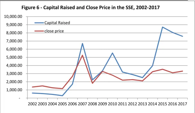
Due to data unavailability, we collected the index and market value of the aggregate SSE market portfolio from 2002 to 2017 (SHANGHAI STOCK EXCHANGE STATISTICS ANNUAL (2005-2008)). We obtained data on annual capitalization and value-weighted price index, and we computed the percentage increase in capitalization and percentage increase in value-weighted price index in each year. Finally, we computed the net dilution ratio for each year, obtaining the annual compounding dilution ratio, amounting to as high as 11.84%. In other words, the increase of market value of total listed companies is 11.84% faster than the increase of market price of the total market portfolio for each of the 16 years. Accordingly, we could find during the 16 years, that the market value of total listed companies increased 12 times from 2.53 trillion Yuan to 33.13 trillion. By contrast, the SSE index increased only 1.44 times, from 1,357.65 to 3,307.17. In 2002, there were 759 listed stocks in the SSE. However, the number of listed companies in the SSE increased to 1440 in 2017. Correspondingly, the capital raised for listed companies increased from 61.43 billion to 757.81 billion from 2002 to 2017. Therefore, there was net creation of new shares because there were too many second placement and IPOs, i.e. many companies capitalize their business with equity.

We also collected the data on capital raised and close prices of the SSE from 2002 to 2017 as shown in the Table 2. In Figure 6 we plot the above data on capital raised and close prices and we can see that the capital raised in the SSE is positively correlated with the SSE price index from 2002 to 2017. The correlation coefficient is as high as 0.79.

(25)

25

Table 2. Capital Raised and Close Price of SSE, 2002-2017

Year Capital Raised

(100 Million Yuan) Close Price 2002 614.30 1,357.65 2003 557.41 1,497.04 2004 456.90 1,266.50 2005 299.77 1,161.06 2006 1,713.51 2,675.47 2007 6,701.33 5,261.56 2008 2,236.85 1,820.81 2009 3,343.15 3,277.14 2010 5,532.14 2,808.08 2011 3,199.69 2,199.42 2012 2,890.31 2,269.13 2013 2,515.72 2,115.98 2014 3,962.59 3,234.68 2015 8,712.96 3,539.18 2016 8,056.45 3,103.64 2017 7,578.06 3,307.17

(26)

26

Source: SHANGHAI STOCK EXCHANGE STATISTICS ANNUAL (2005-2017).

Normally, one would expect that public companies would like to carry IPOs and private placements in the bull market when the SSE index is high, because under this condition they could sell their shares at a decent price, consequently, compared to the bear market, they could finance more liquidity in the bull market. Unlike other security markets which implement registration-based IPO systems, China Security Regulation Commission (CSRC) applies approval-based IPO system in the SSE stock market. The CSRC would like to take advantage of this IPO system to control the stock market, e.g. when the stock market is bearish, the CSRC will postpone the new IPOs or private placements. On the contrary, when the bull market is over-hot that may cause systematically financial risks, the CSRC will accelerate the large scale of IPOs and private placements because they think it will absorb the excess liquidity. Overall, the CSRC treats this system as an assistant of monetary policy. Over the long term, investors consider new IPOs and private placements as a signal that the SSE index will drop. Therefore, in China it is more reasonable to explain that when the SSE index increased sharply, the capital raised approved by CSRC increased dramatically, than when the SSE index drops.

-1,000.00 2,000.00 3,000.00 4,000.00 5,000.00 6,000.00 7,000.00 8,000.00 9,000.00 10,000.00 2002 2003 2004 2005 2006 2007 2008 2009 2010 2011 2012 2013 2014 2015 2016 2017

Figure 6 - Capital Raised and Close Price in the SSE, 2002-2017

Capital Raised close price

(27)

27

Liu, Dang, and Li (2011) show that on the one hand, the increasing SSE index could encourage public companies to finance in the stock market. On the other hand, large scale of financing in the stock market would have negative impacts on the SSE index, and the pressures from excessive financing activities of listed companies can not be neglected. We could also think that a decreasing SSE index would harm the individual investors’ earnings. However, on March 2016, the State Council of China announced China would replace the approval-basis IPO system with a registration-based IPO system systematically in the next 3 years. Therefore, in this paper, we will not consider the decreased equity returns caused by excessive raised capital. Hence, to estimate the growth of earnings that individual investors could obtain, approximately 11% must be deducted from the growth rate of aggregate earnings.

At this point, we have concluded that economic growth places a limit on the growth of the real earning returns per share available for investors over the long term. In accordance with the above analysis, we could reach a conclusion that individual investors could not expect more than a -1% return.

Following up, and as it is known, the equation of returns on common stock per share in period t is:

(8) Rt = ,

where Rt is the common stock return in period t, Pt is the share price at the end of year t, and Dt are the dividends received by investors during period t. More importantly, to better understand the source of the return, we rewrite equation (8): (9) Rt = + Dt /Pt-1=CGt +Dt /Pt-1,

where CGt stands for the capital gains that investors obtained during the period t. Dt /Pt-1 is the dividend yield. Equation (9) expresses the common share returns for one year. but we want to explore the equity returns over the long term. Fama and French (2002) showed that in the long run, the average stock returns (A (R t)) are the average dividend yields plus the average rate of capital gains:

(28)

28

(10) A (R t) = A(Dt /Pt-1) +A(CGt).

Therefore, we have converted the short-term common stock returns equation to a long-term one, and we can estimate the long-term returns on common stock via (10). In addition, A(CGt) could be estimated by our above discussion of no more than -1%.

Cornell (2010) showed that by December 2008, the current dividend yield was 3.1% and the previous 50-year average was 3.3% in the U.S. S&P 500 index portfolio. Comparing to the dividend yield performance of the U.S. S&P 500 index portfolio, the dividend yield of the SSE index portfolio could be almost negligible. Over a long time period, there has been a “Dividend Puzzle” in the Chinese stock market. Because not all the classic dividend theories could explain the dividend practice of Chinese listed companies, regardless of agency theory, signal theory and catering theory. In practice, the majority of Chinese public companies tend to try their best to pay dividends as few as possible or never pay any dividends at all. From 2001, the CSRC started to take measures to solve this problem to protect the interests of public investors. To be more specific, the CSRC has implemented a mandatory dividend policy. Internationally, mandatory standards consider dividend payments as legal obligation. By contrast, the CSRC connects the dividend payments with the financing activities, i.e. if the listed companies do not meet the request on dividend payments, the CSRC will forbid these listed companies to finance in the SSE stock market.

However, listed companies have evaded the mandatory dividend policy. In practice, public companies take advantage of a “fishing strategy”, i.e. they finance a great scale of liquidity from the SSE market by a small amount of dividends as baits. Consequently, not only do they meet the request of mandatory dividend policy, but also achieve the targets of financing.

There might be an internal conflict of the mandatory dividends of CSRC. Because if the public companies pay dividends annually by the request of mandatory dividend policy, they should have liquidity, and then the CSRC should forbid these public companies to finance in the secondary market. By contrast, for companies who, in fact, have profitable projects and lack capital, they are not qualified to finance in the

(29)

29

secondary market because they do not have enough cash to pay dividends. Alternatively, if they first pay dividend to shareholders in order to finance in the secondary market, the investing opportunities are far more likely to disappear when they finish financing in the secondary market.

Yang and Wang (2017) showed that overall the dividend yield of Chinese listed companies is quite low, 59% of the public companies’ dividend yields are in the interval from 0 to 1%, 27% of the public companies’ dividend yields are in the interval from 1% to 2%, and only 14% of the listed companies’ dividend yields are larger than 2% from 1990 to 2015. The dividends’ yield of most of the listed companies are lower than the bank deposit interest rate over one-year in China. The average dividend yields increased from 0.02% to 0.48% in 2015. Therefore, we could not expect the dividend yield in the SSE market to be more than 0.5% in the future unless there are some economic innovations and economic reforms from the CSRC.

5. Conclusion

In the long-run, economic growth is destined to cap the revenues growth of all the business participators. Because of the fundamental relation between revenues and earnings, economic growth determines the earnings’ growth. Public companies are constrained to this rule as well. As the most important fundamental information, the changes in the earnings will eventually be reflected in the share price, thus have impact on equity returns.

In this paper we have used the theoretical framework of Cornell (2010), taking into consideration of convergence because the 9% real growth rate in China includes both technology progress and “catch-up” effect, and extending the research scope from developed countries to emerging countries. We have applied this methodology to the largest emerging country i.e. China.

Empirically, we have found that the long run expected equity return in China should not be more than -0.5 percent. Cornell (2010) concluded that over the long run, investors should anticipate real returns on shares to average no more than 4 percent in

(30)

30

the U.S.. We could observe that the real returns on common stocks in China is far less than that in the U.S., although real GDP per capital growth in China is much higher. As we reported in our analysis, the most important reason is the dilution effect caused by net creation of new shares.

Summarising, we have used the average real growth rate of per capita GDP in China from 1990 to 2017 to estimate technology progress effect and the convergence effect, which contributes 9% to equity returns. In addition, we have used the average population growth in China from 1990 to 2017 to estimate its contribution, of around 1%, to equity returns. In the line of Bernstein and Arnott (2003), we have considered a dilution effect of 11% that was caused by the net creation of new shares. Finally, we have considered the impacts of dividend yield, and the observed dividend yield in China can not contribute more than 0.5% to equity returns. Thus, we find that the long-run real expected return for the SSE common stocks is -0.5%. The primary reason for such result is the dilution effect.

References

Barro, Robert J., and Peter Jose F. Ursua. 2008. Macroeconomic Crises since 1870. NBER Working Paper 13940 (April).

Cornell, B. 2010, Economic Growth and Equity Investing, Financial Analysts Journal, pp.54-64.

Campbell, John Y., and Robert J. Shiller. 1998. “Valuation Ratios and the Long-Run Stock Market Outlook.” Journal of Portfolio Management, vol. 24, no. 2 (Winter):11 –26.

Central Intelligence Agency. 2008. The 2008 World Fact Book. Washington, DC: Central Intelligence Agency.

David Romer 2012, ADVANCED MACROECONOMICS, Fourth Edition, pp.16-18. Eugene F.Fama and Kenneth R.French 2002, The Equity Premium, The Journal of Finance Vol 57, NO.2 April 2002, pp.637-659

LIU De-hong, DANG M in, LI Tao 2011, An Empirical Study of the Correlation of SSE Composite and A-share Market Financing, Journal of Beijing Jiaotong

(31)

31

University( Social Science Edition), Vol.10,No.3,Jul.2011, pp.78-83.

Liu Yuping, The Mechanism of bubble’s appearance and expansion. Journal of Nanchang University, 2006 (11).

Robert M.Solow 1956, A Contribution to the Theory of Economic Growth, the Quarterly Journal of Economics, Vol.70, No. 1(Feb.,1956), pp.65-94.

Robert D. Arnott and Peter L.Bernstein 2001, What Risk Premium Is “Normal”? , Financial Analysts Journal, pp.64-85.

Su Dongwei, Wu Yangru, The Sustainable Development of China’s Listed Firms: Econometric Model and Empirical Evidence, Economic Research, pp.106-116 Nicholson, S.F. 1960, Price-earnings ratios, Financial Analysts Journal, Vol.16, no.4, pp. 43-45

Weil, David N. 2009. Economic Growth. 2nd ed. Boston: Addison Wesley.

YANG Bao and WANG Yihan 2017, The Statistical Traits Chinese Listed Firms’ Cash Dividend Policy: An Examination of 1990-2015 Dividend Yield, Journal of Chongqing University of Technology (Social Science) Vol.31 No.12 2017.pp.71-79. Yi Xianrong, Bubble have been blown, Guangzhou Daily, 25-01-2017.

Zhao Xiao, It’s Better to Control the Bubble at the Beginning. Shanghai Securities News, 07-03-2007.

Data sources

Huang Hongyuan, SHANGHAI STOCK EXCHANGE STATISTICS ANNUAL (2013), Shanghai People′s Publishing House.

Huang Hongyuan, SHANGHAI STOCK EXCHANGE STATISTICS ANNUAL (2016), Shanghai Far East Publishers.

(32)

32

Huang Hongyuan, SHANGHAI STOCK EXCHANGE STATISTICS ANNUAL (2017), Shanghai Far East Publishers.

Zhu Congjiu, SHANGHAI STOCK EXCHANGE STATISTICS ANNUAL (2005), Shanghai People′s Publishing House.

Zhang Yujiu, SHANGHAI STOCK EXCHANGE STATISTICS ANNUAL (2008), Shanghai People′s Publishing House.

Economic growth and equity returns : application to the chinese stock market

M

ONETARY AND

M

ASTER

ECONOMIC GROWTH AND

APPLICATION TO THE CHIN

Y

ULIN

A

N

S

:

A

A

ONETARY AND

F

INANCIAL

E

CONOMICS

ASTER

´

S

F

INAL

W

ORK

D

ISSERTATION

ECONOMIC GROWTH AND EQUITY RETURNS:

LICATION TO THE CHINESE STOCK MARKET

D

ECEMBER

2018

CONOMICS

EQUITY RETURNS:

ESE STOCK MARKET

Contents