Cândida Ferreira Bank performance and economic growth: evidence from Granger panel causality estimations

(1)

Carlos Pestana Barros & Nicolas Peypoch

A Comparative Analysis of Productivity Change in Italian and Portuguese Airports

WP 006/2007/DE _________________________________________________________

Cândida Ferreira

Bank performance and economic growth: evidence from Granger panel causality estimations

WP 21/2013/DE/UECE _________________________________________________________

De pa rtme nt o f Ec o no mic s

WORKING PAPERS

ISSN Nº 0874-4548

(2)

Bank performance and economic growth: evidence from Granger panel causality

estimations

Cândida Ferreira [1]

Abstract

This paper provides empirical evidence on the causality relations between bank performance and economic growth in a panel including 27 European Union member-states from 1996 through to the onset of the 2008 financial crisis. Bank performance is represented not only by the Return on Assets (ROA) and Return on Equity (ROE) ratios but also by bank cost efficiency, measured through Data Envelopment Analysis (DEA). For economic growth, we consider not only the GDP per capita but also the gross fixed capital formation growth. Deploying a panel Granger causality approach, we confirm positive causality running from bank performance to economic growth. However, as regards the opposite causality, running from growth to bank performance, we conclude that economic growth positively contributes to the bank ROA and ROE ratios but not so certainly in the case of the DEA bank cost efficiency.

Keywords: Bank performance, Economic growth, DEA, Panel Granger causality, European Union. JEL Classification: G21, G31, E44, F43, F36,

[1]_{ISEG-UTL - Instituto Superior de Economia e Gestão – Technical University of Lisbon}

and UECE – Research Unit on Complexity and Economics Rua Miguel Lupi, 20, 1249-078 - LISBON, PORTUGAL tel: +351 21 392 58 00

(3)

Bank performance and economic growth: evidence from Granger panel causality

estimations

1. Introduction

The contribution of financial development to economic growth has been extensively analysed and empirically tested in recent decades and most especially after the King and Levine (1993) contribution.

In spite of controversy over the variables introduced to represent financial development and the appropriate estimation techniques, most empirical studies do conclude that financial development promotes economic growth and advocating that a smoothly functioning financial sector contributes to the mobilization of savings, the diversification of risk and a better allocation of financial resources. Although less analysed, there is also a strand of literature (represented by Greenwood and Bruce, 1997, among others) that studies the inverse relationship and thereby approaching how economic growth fosters financial development because growth in the real economy increases demand for financial services and thus contributes to the sector’s development.

Hence, in spite of the fact that many authors concur on the actual importance of the relationship between financial development and economic growth, the direction of causality still remains a controversial issue.

(4)

for portraying economic growth (such as bank credits, deposits or bank liabilities). Their conclusions differ whether in terms of the kind of countries, the time interval considered and the variables applied but, generally speaking, they confirm that the causality running from financial development to economic growth proves easier to demonstrate than the opposite causality running from economic growth to financial development.

This paper seeks to contribute to the debate on the causality relationship between finance and growth using a panel Granger causality approach and departing from recent empirical work in order to complement the evidence existing, especially in the following terms:

 We consider a panel including the 27 European Union member states over a relatively long timeframe, from 1996 through to the onset of the 2008 financial crisis;

 We take into account the dominant role of banking institutions in the European financial sector and instead of using traditional proxies for representing financial development, we test the specific relationship between bank performance and economic growth;

 We approach bank performance by the usual Return on Assets (ROA) and Return on Equity (ROE) ratios in addition to measures of bank efficiency obtained by Data Envelopment Analysis (DEA);

 For economic growth, we consider not only the commonly applied per capita Gross Domestic Product (GDP) but also the investment channelled into growth in addition to the gross fixed capital formation.

(5)

This paper is structured as follows: Section 2 presents the relevant literature, section 3 explains the methodological framework and data sample; Section 4 reports the empirical results obtained; Section 5 concludes.

2. Relevant literature

The link between economic growth and the quality of financial systems dates back at least as far as Schumpeter (1911), who maintained that the services provided by financial intermediaries prove essential to economic innovation, productive investment and economic growth. Over the last century, this question has been subject to theoretical debates and empirical studies, which rose in particular in the wake of the renowned King and Levine (1993) paper.

According to most studies, financial development plays an important role in economic growth as well-functioning markets and financial institutions are identified as decreasing transaction costs and problems over asymmetric information levels. At the same time, financial institutions act to identify investment opportunities by selecting the most profitable projects, mobilizing savings, facilitating trade and the diversification of risk while also improving corporate governance mechanisms.

(6)

A few years later, Beck et al. (2004) deployed the ratio between credits from financial intermediaries to the private sector divided by GDP as a proxy to capture the depth and breadth of financial intermediation in a panel of 52 countries over the period 1960 to 1999. They conclude that financial development is not only clearly pro-growth but also pro-poor, thus, in countries with better-developed financial intermediation, income inequality declines more rapidly.

Providing a review of the literature and the empirical evidence on the relationship between financial development and economic growth, Khan and Senhadji (2000) conclude that the results of empirical studies analysing the relationship between financial development and economic growth indicate that, while the general effects of financial development on the outputs may be positive, the size of these effects varies not only with the different variables considered, the financial development indicators but also with the estimation method, data frequency or the defined functional form of the relationship. On the other hand, there are authors like Stiglitz (1985), Bhide (1993), Bencivenga et al. (1995), who stressed that certain costs may stem from the role of financial intermediaries and correspondingly these intermediaries may also sometimes be subject to adverse selection and moral hazard problems that may constrain real economic growth through inhibiting resource allocation, exaggerating fluctuations in interest rates, or contributing to falls in the saving rates prevailing.

Other authors, including Loayza and Rancière (2006), underline the importance of the time horizon, defending that, in the long term, the literature on economic growth finds a positive relationship between financial development and growth but, in the short term, the literature mostly on bank crises returns a negative relationship and concludes that monetary aggregates may represent good predictors of economic crisis.

(7)

in focusing on advanced economies, these authors demonstrate that a fast-growing financial sector is detrimental to aggregate productivity growth.

Ayadi et al. (2013) use a sample of northern and southern Mediterranean countries for the 1985-2009 time period and conclude there are deficiencies in bank credit allocation in these countries as credit to the private sector and bank deposits are negatively associated to economic growth; however, on the stock market side, the results indicate that stock market size and liquidity do contribute to growth. Furthermore, these authors conclude both that poorer countries are catching up with richer countries in terms of GDP growth and that low inflation and the quality of institutions are key factors to growth. Rajan and Zingales (1998) had already pointed out that the positive correlation usually returned by financial development and economic growth might derive from a problem of omitted variables. They argued that there is no clear causality between financial development and economic growth and proposed further tests to analyse the mechanism through which financial development may promote economic growth taking into account both the country and sectorial effects. Thus, rather than adhering to the traditional explanation of economic growth by proxies of financial development, Rajan and Zingales (1998) test the hypothesis that financial markets and banking institutions not only reduce the cost of financing but also help to combat problems provoked by asymmetrical information and correspondingly assuming in their test that those sectors most dependent on external financing represent those growing at the fastest pace and in line with the development of the financial markets and institutions to which these sectors have access.

(8)

conclusion that world output might increase by 53 per cent if all countries adopt the best global financial practices.

Koetter and Wedow (2010) study the importance of financial intermediation by banks to the economic growth taking place in 97 German economic planning regions between 1993 and 2004 and conclude

that the quality of these banks, as reported by bank cost efficiency, robustly contributes to growth,

while the quantity of bank credit provided does not clearly correlate with economic growth. The same

kind of conclusions are obtained by Hasan et al. (2009) who study whether regional growth in eleven

European countries gets influenced by bank costs and profit efficiency over the time period

1996-2005. Their findings indicate how, in these countries, an increase in bank efficiency generates five

times more influence on economic growth than the same rise in the level of bank credit provided.

There is also a strand of the literature represented by authors like Robinson (1952), Gurley and Shaw (1967), Goldsmith (1969), Jung (1986), Greenwood and Jovanovic (1990), Berthelemy and Varoudakis (1996), Greenwood and Bruce (1997) who remain unconvinced as to the one-way causality of financial development on economic growth and postulate that there may be a reverse causality between economic growth and financial development. Furthermore, other authors even assume that the relationship between financial development and economic growth represents a two-way causality (among others, Patrick, 1966; Demetriades and Hussein, 1996; Blackburn and Hung, 1998; Luintel and Khan, 1999; Khan, 2001; Shan et al., 2001; Calderon and Liu, 2003).

(9)

impact of financial development on economic growth thereby positing that the effect of financial sector deepening on the real economy requires time to become evident while furthermore finding that even though financial development may enhance economic growth through both capital accumulation and productivity growth, the productivity channel would seem a stronger influence.

More recently, Hassan et al. (2011) study how financial development links to economic growth through applying Granger causality tests for a sample period between 1980 and 2007, and categorizing low and middle income countries into six geographic regions: East Asia and the Pacific, Europe and Central Asia, Latin America and the Caribbean, Middle East and North Africa, South Asia, Sub-Saharan Africa; and also two groups of high-income countries: OECD and non-OECD countries. Their findings point to the conclusion favouring evidence on the role of financial development in economic growth in low and middle income countries. More precisely, in the short run, there is two-way causality between financial development and economic growth, reported in all regions apart from Sub-Saharan Africa and East Asia and the Pacific. However, these latter two regions have causality running from economic growth to financial development supporting the hypothesis that in developing countries growth leads finance because of the increasing demand for financial services.

(10)

For a panel of fifteen Southern and Eastern Mediterranean countries, and the 1980-2007 time span, Kar et al. (2011) conclude that the causality between finance and economic growth mostly depends on the measurement of financial development and differs from country to country.

Abdelhafidh (2013) returned the same kind of conclusion following analysis on the direction of causality interactions between finance and growth in a sample of North African countries for the 1970-2008 time period. The general conclusion is that Granger economic growth raises domestic savings in these countries even though the findings point to specific country results, with unilateral and sometimes bilateral Granger causality relations between the different proxies for financial development and economic growth. They also underscore the policy implications of different financial sources on economic growth and the merits of a case by case approach.

3. Methodological framework and datasample

In order to test the causality relationship between bank performance and economic growth we follow here the Granger causality concept (Granger, 1969) and the approaches developed to analyse the existence of causality relationships among variables in panels (by such authors as Holtz-Eakin et al., 1988; Weinhold, 1996; Nair-Reichert and Weinhold 2001; Kónya, 2006; Hurlin and Venet, 2008; Bangake and Eggoh, 2011), using the general linear panel Granger causality model:

(1) , 1 , ) ( 1 , ) (

, it

K k k t i k i K k k t i k i t

i y x

y













       

Where: y = dependent variable; x = explanatory variable; i = 1,...,N cross units; t = 1,...,T time periods;

(11)

To test Granger non-causality from x to y, the null hypothesis is H_o :



_i 0,i1,...,N

The alternative hypothesis states that there is a causality relationship from x to y for at least one

cross-unit of the panel: ₁: 0, 1,..., ₁; 0,  ₁1, ₁2..., ;(0 1 1) N N N

N N i N

i

H _i _i .

Our sample comprises a panel in which the cross units are 27 EU countries (i = 1, …, 27) and the timeframe covers a relatively long period, from 1996 to the onset of the 2008 financial crisis (t = 1996, …, 2008).

Over the following pages, we set out the variables chosen to represent bank performance (return on assets, return on equity and bank cost efficiency) and economic growth (considering not only per capita GDP but also gross fixed capital formation). We also report the results of the unit root tests of the series studied.

3.1. Bank performance

We measure bank performance through two of the ratios commonly applied to analyse the banking sector performance: the return on assets (ROA) and the return on equity (ROE); we also consider a measurement for bank efficiency (generated by Data Envelopment Analysis). All data for these three bank performance variables are sourced from the IBCA-BankScope 2008 CD (annual data from the consolidated accounts of commercial and saving banks, all in nominal values and in Euros).

(12)

The ROA is the ratio of the net income to the total bank assets and serves to assess the efficiency of bank resource applications and their respective financial strength. Bank net income in itself provides a good indication of the bank’s overall performance even while suffering from one important drawback: it does not take into account the bank’s size and thereby rendering comparisons among different banking institutions and/or different time periods difficult.

The use of ROA (and also of ROE) adjusts in accordance with the size of banks and thereby making possible those comparisons among institutions for the same or for different time periods. Thus, the ROA is a simple measure of bank profitability providing a good insight into just how well, or otherwise, the bank management is doing its job through reflecting the performance of the bank’s assets in terms of the profits returned.

Appendix A presents the ROA obtained for our sample of the 27 EU member state banking institutions countries between 1996 and 2008. The results also demonstrate the clear difficulties faced by banking institutions in some important EU countries in 2008. For the years leading up to 2008, there are few negative results and only in some new EU member states and during some critical years in Germany’s reunification process. Nevertheless, generally speaking, for the time period between 1996 and 2007, our ROA results reveal a general tendency towards rising profits generated by bank assets in most EU countries.

Return on equity

(13)

Appendix B contains the results returned for ROE in our sample that confirm the clear difficulties encountered by banking institutions in some leading EU countries in 2008 and a few negative values for banking institutions in some new EU members and the reunified Germany. However, there is no clear trend in the rises and falls in the ROE results for the years before 2008. On the contrary, these ROE results report clear oscillations in the ratio of bank earnings and shareholder equity investment across the 27 EU countries.

Bank cost efficiency

To measure bank efficiency we adopted the Data Envelopment Analysis (DEA), a non-parametric method developed by, among others, Coelli et al. (1998), Thanassoulis (2001) and Thanassoulis et al. (2007). Here, we take the intermediation approach considering that total bank costs depend on three bank outputs: total loans, total securities and other earning assets; and also on three bank inputs: borrowed funds, physical capital and labour. Our sample comprises annual data from the consolidated accounts of commercial and saving banks from 27 EU countries between 1996 and 2008, sourced from the IBCA-BankScope 2008 CD.

(14)

3.2. Economic growth

Economic growth will be represented by the Gross Domestic Product (GDP) but also by the gross fixed capital formation, taking into account the importance of the fixed capital to create necessary conditions to economic growth. The used data were sourced from the Eurostat statistical database and defined in nominal terms (as were also defined the bank performance variables, sourced from the IBCA-BankScope 2008 CD).

Gross domestic product

In our estimations we apply per capita nominal GDP at market prices (Euro per inhabitant) sourced from the Eurostat statistical database. The data reported in Appendix D demonstrate that during the period considered nominal per capita GDP rose throughout the 27 EU countries, and grew at its fastest pace in countries with lower GDP levels (for instance, around five times more in Bulgaria and in the Czech Republic) even though this increased growth did not amount to eliminating the enormous discrepancies still persisting among the 27 countries.

Gross fixed capital formation

(15)

3.3. Unit root tests

The number of observations in our panel (27 countries x 13 annual observations) does not lend itself to the application of single-unit root tests for time series. Therefore, we opted for panel-unit root tests, which prove more appropriate to this case. These tests not only increase the power of unit root testing due to the observation span but also minimise the risks of structural breaks.

From among the available panel unit root tests, we chose here to use the Levin, Lin and Chu (2002) test and the Im, Pesaran and Shin (2003) test.

The Levin, Lin and Chu (2002) may be viewed as a pooled Dickey-Fuller test, or as an augmented Dickey-Fuller test, which include lags and the null hypothesis stems from the existence of non-stationarity. This test is adequate for moderate size, heterogeneous panels and such as the panels applied in this paper with fixed effects, and assumes there is a common unit root process. The results reported in Appendix F enable us to reject the existence of the null hypothesis.

The Im, Pesaran and Shin (2003) test estimates the t-test for unit roots in heterogeneous panels and allows for individual unit root processes. This involves applying the mean of the individual Dickey-Fuller t-statistics to each panel unit and assumes that all series are non-stationary under the null hypothesis. Appendix G presents the results obtained with this test, and they confirm the rejection of non-stationarity.

4. Empirical results

(16)

Return on Equity, ROE, ratios and also by bank cost efficiency level as measured through Data Envelopment Analysis, DEA).

We opted to deploy both panel ordinary least squares (OLS) estimations and fixed-effects panel estimations, in keeping with Wooldridge (2002) and Baltagi (2008), among others and first present the results obtained for the causality running from bank performance to growth and then the inverse causality running from growth to bank performance.

4.1. Causality running from bank performance to growth

Table 1 feature the obtained results for the causality running from bank performance to economic growth generated by panel ordinary least square (OLS) robust estimations and panel fixed robust estimations.

As regards GDP per capita, Tables 1-A, 1-B and 1-C report the specific influence of the variables representing bank performance (respectively, the ROA and ROE ratios and also DEA bank cost efficiency). In all situations, the results obtained confirm the positive effect of all these variables on GDP growth, and these effects are statistically strong at least for the first lags of bank performance variables.

Simultaneously, and also as expected, as we are dealing with panel estimations, the R-squared values returned are not remarkable. Nevertheless, for the fixed-effects estimations, the R-squared obtained for “between” are not only relatively high but also always much higher than the R-squared “within”, revealing how for the panel considered, the cross-section evolution (“between” the countries) is always stronger than the time evolution (“within” the interval considered).

(17)

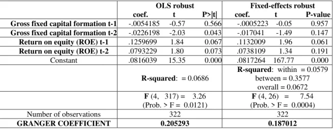
More precisely, in all situations, there is a clear and positive influence of ROA (Table 1-D), ROE (Table 1-E) and bank cost efficiency (Table 1-F) on the growth of the gross fixed capital formation, and these results are statistically stronger for the first lags of the bank performance variables. Furthermore, and also in line with the previous results, the R-squared values obtained enable us to conclude that the cross-section evolution between the 27 EU countries is more relevant in this panel than the time evolution during the interval considered (1996-2008).

A more careful comparison of the information reported in Table 1 clearly demonstrates that the best results are obtained in Table 1 – F, demonstrating that with both robust OLS and panel-fixed robust estimations, bank cost efficiency exerts a statistically strong positive influence on the growth in gross fixed capital formation.

(18)

TABLE 1 – CAUSALITY RUNNING FROM BANK PERFORMANCE TO ECONOMIC GROWTH

Table 1 - A - Dependent variable: Gross domestic product at market prices (Euro per inhabitant); explanatory variable: Return on assets (ROA)

OLS robust

coef. t P>|t|

Fixed-effects robust coef. t P-value GDP per capita t-1 -.02102 -2.00 0.046 -.0137797 -1.36 0.187 GDP per capita t-2 -.0093003 -1.42 0.156 -.0013958 -0.33 0.744 Return on assets (ROA) t-1 .8580076 1.49 0.137 .8257388 2.31 0.029 Return on assets (ROA) t-2 .030947 0.08 0.934 -.0058706 -0.02 0.986

Constant .070038 21.49 0.000 .0701304 532.72 0.000

R-squared: = 0.0730

R-squared: within = 0.0757 between = 0.2929

overall = 0.0686 F (4, 317) = 3.96

(Prob. > F = 0.0038)

F(4, 26) = 27.82 (Prob. > F = 0.0000)

Number of observations 322 322

GRANGER COEFFICIENT 0.888955 0.819868

Table 1 - B - Dependent variable: Gross domestic product at market prices (Euro per inhabitant); explanatory variable: Return on equity (ROE)

OLS robust

coef. t P>|t|

Fixed-effects robust coef. t P-value GDP per capita t-1 -.0215765 -2.00 0.046 -.014548 -1.48 0.151 GDP per capita t-2 -.0093493 -1.43 0.153 -.0015179 -0.33 0.742 Return on equity (ROE) t-1 .0769428 1.81 0.072 .0714988 2.49 0.020 Return on equity (ROE) t-2 .0167438 0.59 0.553 .0134006 0.51 0.614 Constant .0697435 21.26 0.000 .0698698 288.58 0.000

R-squared: = 0.0752

overall = 0.0712 F (4, 317) = 4.50

(Prob. > F = 0.0015)

F (4, 26) = 49.48 (Prob. > F = 0.0000)

Table 1 - C - Dependent variable: Gross domestic product at market prices (Euro per inhabitant); explanatory variable: Cost Efficiency (DEA)

OLS robust

coef. t P>|t|

Fixed-effects robust coef. t P-value GDP per capita t-1 -.0289362 -2.92 0.004 -.0216277 -2.55 0.017 GDP per capita t-2 -.011864 -1.44 0.152 -.0040334 -0.56 0.582 Cost Efficiency (DEA) t-1 .0500286 2.47 0.014 .0393857 1.71 0.100 Cost Efficiency (DEA) t-2 .0229764 1.36 0.173 .0134193 0.66 0.518 Constant .0699159 21.88 0.000 .07013 287.42 0.000

R-squared: = 0.0810

overall = 0.0783 F (4, 317) = 4.45

(Prob. > F = 0.0016)

F (4, 26) = 2.09 (Prob. > F = 0.1114)

(19)

Table 1 - D - Dependent variable: Gross fixed capital formation; explanatory variable: Return on assets (ROA)

OLS robust

coef. t P>|t|

Fixed-effects robust coef. t P-value Gross fixed capital formation t-1 -.0051933 -0.56 0.576 -.0001781 -0.02 0.986 Gross fixed capital formation t-2 -.0237701 -2.18 0.030 -.0182414 -1.67 0.107 Return on assets (ROA) t-1 1.156915 1.41 0.160 1.054623 1.35 0.190 Return on assets (ROA) t-2 .4841011 0.83 0.409 .4258303 0.82 0.418 Constant .0822218 15.42 0.000 .0822752 244.77 0.000

R-squared: = 0.0560

overall = 0.0547 F (4, 317) = 2.22

(Prob. > F = 0.0662)

F (4, 26) = 4.81 (Prob. > F = 0.0040)

Table 1 - E - Dependent variable: Gross fixed capital formation; explanatory variable: Return on equity (ROE)

OLS robust

coef. t P>|t|

Fixed-effects robust coef. t P-value Gross fixed capital formation t-1 -.0054185 -0.57 0.566 -.0005223 -0.05 0.957 Gross fixed capital formation t-2 -.0226198 -2.03 0.043 -.017041 -1.49 0.147 Return on equity (ROE) t-1 .1259699 1.84 0.067 .1132009 1.96 0.061 Return on equity (ROE) t-2 .0793229 1.80 0.073 .0738109 1.34 0.191 Constant .0816039 15.35 0.000 .0817264 167.77 0.000

R-squared: = 0.0686

overall = 0.0672 F (4, 317) = 3.26

(Prob. > F = 0.0121)

F (4, 26) = 7.54 (Prob. > F = 0.0004)

Table 1 - F - Dependent variable: Gross fixed capital formation; explanatory variable: Cost Efficiency (DEA)

OLS robust

coef. t P>|t|

Fixed-effects robust coef. t P-value Gross fixed capital formation t-1 -.0124428 -2.02 0.044 -.0071564 -0.95 0.353 Gross fixed capital formation t-2 -.0271697 -2.51 0.013 -.0217012 -2.55 0.017 Cost Efficiency (DEA) t-1 .1181437 4.20 0.000 .1068434 3.26 0.003 Cost Efficiency (DEA) t-2 .0637245 2.60 0.010 .0527886 1.94 0.064 Constant .0815758 15.80 0.000 .0817325 259.91 0.000

R-squared: = 0.1091

overall = 0.1079 F (4, 317) = 7.35

(Prob. > F = 0.0000)

F (4, 26) = 4.82 (Prob. > F = 0.0048)

(20)

4.2. Causality running from growth to bank performance

The results returned for the causality running from economic growth to bank performance, and also applying panel OLS robust estimations and fixed-effects robust estimations, are detailed in Table 2.

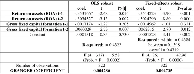
More precisely, in the first half of this table we report the results for the influence of GDP per capita growth on the three bank performance variables: on Return on Assets (Table 2 – A), on Return on Equity (Table 2 – B) and on bank cost efficiency (Table 2 – C). In the final section of Table 2 (that is, Table 2 – D, Table 2 – E and Table 2 – F), we set out the results obtained for the influence of gross fixed capital formation on ROA, ROE and bank efficiency respectively.

In all situations, the resulting R-squared values presented in Table 2 are much higher than those for the causality running from bank performance to growth reported in Table 1. Furthermore, and also contrary to Table 1, for the fixed-effects estimations we obtain a much stronger R-squared “within” result than that for the R-squared “between” and therefore reach the conclusion that for the causality running from growth to bank performance the time evolution (“within” the considered interval, 1996-2008) is much more relevant than the cross-section evolution (“between” the 27 EU countries included in the panel).

In addition, for all the explanatory variables, the results obtained are statistically valid (and much stronger) for the second lags than for the first, confirming the relevance of time delays to this process as the effects of economic growth on bank performance are not immediate.

(21)

results of the second lags positive and statistically relevant but also the joint-influence of the two lags under consideration, represented by the correspondent causality Granger coefficients, always proves positive.

On the other hand, for the causality running from economic growth to bank cost efficiency, the results obtained when growth is proxied by GDP per capita (Table 2 – C) and when proxied by gross fixed capital formation (Table 2 – F), while not very strongly in statistical terms, generally turn out negative.

To understand this possible non-alignment between economic growth and bank efficiency, we should recall that DEA efficiency is a relative measure, dependent on the chosen sample and, in our estimations, we considered that bank costs depend on the combinations of three bank outputs (total loans, total securities and other earning assets) and three bank inputs (borrowed funds, physical capital and labour).

Hence, it would not prove difficult to accept that, for our panel of EU countries, over the time period considered, these combinations of outputs and inputs depend on many factors other than economic growth.

(22)

TABLE 2 – CAUSALITY RUNNING FROM ECONOMIC GROWTH TO BANK PERFORMANCE

Table 2-A - Dependent variable: Return on assets (ROA); explanatory variable: Gross domestic product at market prices (Euro per inhabitant)

OLS robust

coef. t P>|t|

Fixed-effects robust coef. t P-value Return on assets (ROA) t-1 -.3484563 -2.56 0.011 -.3473012 -4.00 0.000 Return on assets (ROA) t-2 -.2684678 -3.06 0.002 -.2684267 -10.54 0.000 GDP per capita t-1 -.0038217 -1.46 0.146 -.0035203 -1.27 0.214 GDP per capita t-2 .0088773 2.75 0.006 .0091956 2.84 0.009 Constant -.0001383 -0.32 0.752 -.0001357 -2.54 0.017

R-squared: = 0.4224

overall = 0.4221 F (4, 317) = 5.99

(Prob. > F = 0.0001)

F (4, 26) = 28.85 (Prob. > F = 0.0000)

Table 2-B - Dependent variable: Return on equity (ROE); explanatory variable: Gross domestic product at market prices (Euro per inhabitant)

OLS robust

coef. t P>|t|

Fixed-effects robust coef. t P-value Return on equity (ROE) t-1 -.3498541 -1.94 0.053 -.3495838 -4.00 0.000 Return on equity (ROE) t-2 -.230413 -2.05 0.041 -.2290209 -9.01 0.000 GDP per capita t-1 -.0222006 -1.06 0.290 -.0180974 -0.96 0.348 GDP per capita t-2 .0895546 2.29 0.023 .0942303 2.50 0.019 Constant -.0029979 -0.43 0.667 -.0029558 -3.00 0.006

R-squared: = 0.2805

overall = 0.2802 F (4, 317) = 4.72

(Prob. > F = 0.0010)

F (4, 26) = 22.91 (Prob. > F = 0.0000)

Table 2 - C - Dependent variable: Cost Efficiency (DEA); explanatory variable: Gross domestic product at market prices (Euro per inhabitant)

OLS robust

coef. t P>|t|

Fixed-effects robust coef. t P-value Cost Efficiency (DEA)t-1 -.0861809 -1.26 0.210 -.1111668 -2.67 0.013 Cost Efficiency (DEA)t-2 -.1639728 -1.89 0.060 -.1857853 -3.43 0.002 GDP per capita t-1 -.001682 -0.05 0.958 .007362 0.27 0.786 GDP per capita t-2 -.0931096 -1.75 0.082 -.0844469 -1.64 0.112

Constant -.0051778 -0.61 0.540 -.0047732 -10.53 0.000

R-squared: = 0.1181

overall = 0.1157 F (4, 317) = 2.53

(Prob. > F = 0.0408)

F (4, 26) = 10.85 (Prob. > F = 0.0000)

(23)

Table 2 - D - Dependent variable: Return on assets (ROA); explanatory variable: Gross fixed capital formation

OLS robust

coef. t P>|t|

Fixed-effects robust coef. t P-value Return on assets (ROA) t-1 -.3531667 -2.48 0.014 -.3514223 -3.90 0.001 Return on assets (ROA) t-2 -.3034327 -3.15 0.002 -.3024296 -8.80 0.000 Gross fixed capital formation t-1 -.0017174 -1.27 0.205 -.0014962 -1.01 0.321 Gross fixed capital formation t-2 .0060029 2.73 0.007 .0062315 2.70 0.012

Constant -.0001518 -0.35 0.730 -.0001523 -3.41 0.002

R-squared: = 0.4322

overall = 0.4319 F (4, 317) = 5.58

(Prob. > F = 0.0002)

F (4, 26) = 42.96 (Prob. > F = 0.0000)

Table 2 - E - Dependent variable: Return on equity (ROE); explanatory variable: Gross fixed capital formation

OLS robust

coef. t P>|t|

Fixed-effects robust coef. t P-value Return on equity (ROE) t-1 -.3541566 -2.02 0.044 -.3517636 -3.84 0.001 Return on equity (ROE) t-2 -.2484065 -2.25 0.025 -.2452814 -8.67 0.000 Gross fixed capital formation t-1 -.0092782 -0.86 0.391 -.0055061 -0.56 0.579 Gross fixed capital formation t-2 .0665872 2.38 0.018 .0705989 2.46 0.021

Constant -.00316 -0.46 0.647 -.0031785 -3.61 0.001

R-squared: = 0.3129

overall = 0.3123 F (4, 317) = 4.88

(Prob. > F = 0.0008)

F (4, 26) = 30.38 (Prob. > F = 0.0000)

Table 2 - F - Dependent variable: Cost Efficiency (DEA); explanatory variable: Gross fixed capital formation

OLS robust

coef. t P>|t|

Fixed-effects robust coef. t P-value Cost Efficiency (DEA) t-1 -.0866303 -1.26 0.208 -.1144128 -2.68 0.013 Cost Efficiency (DEA) t-2 -.1592579 -1.69 0.091 -.1824269 -2.87 0.008 Gross fixed capital formation t-1 -.0026062 -0.17 0.864 -.0001657 -0.01 0.991 Gross fixed capital formation t-2 -.0414804 -1.35 0.177 -.0396671 -1.30 0.205 Constant -.00474 -0.54 0.588 -.004398 -9.82 0.000

R-squared: = 0.0829

overall = 0.0818 F (4, 317) = 2.39

(Prob. > F = 0.0507)

F (4, 26) = 9.02 (Prob. > F = 0.0001)

(24)

4.3. Granger coefficients and F-tests results

In Table 3, we present a summary of the values obtained with OLS robust and fixed-effects robust estimations for the causality Granger coefficients and the F tests (always supposing the joint hypothesis 1 = 2 = 0). In Part I of Table 3 we put forward the results for causality running from

bank performance to economic growth before the results for inverse causality, from growth to bank performance, in Part II.

The F-test results underpin the conclusion that, in general, our estimations are statistically significant for bi-directional causality relations between growth and bank performance.

The reported values of the Granger coefficients clearly confirm the positive causality between bank performance (here represented by the ROA and ROE ratios and bank cost efficiency) and economic growth. These results are in line with the literature defending how the best financial practices nurture economic growth (for instance, recently, Greenwood et al. 2013) and very particularly with the conclusions from such authors as Koetter and Wedow (2010) or Hasan et al. (2009), who have analysed the importance of bank efficiency to growth in some EU countries for time intervals ranging from the mid-1990s through to the mid-2000s.

(25)

section of Table 3, we may conclude in favour of clear and positive bi-directional panel Granger causality between growth and bank performance.

However, as regards the influence of economic growth on bank efficiency, the Granger coefficients presented in Table 3 do not provide for any conclusion as to growth bringing about an increase in bank efficiency.

(26)

TABLE 3 – GRANGER COEFFICIENTS AND F-TESTS RESULTS

Part I Part II

OLS robust Fixed effects robust

1-A Dep. var: GD per capita; expl.var:

Return on assets (ROA)

0.888955

F (4, 317) = 3.96 (Prob. > F =

0.0038)

0.819868

F(4, 26) = 27.82 (Prob. > F =

0.0000)

2-A Dep. var:

Return on assets (ROA); expl.var:

GDP per capita

0.005056

F (4, 317) = 5.99 (Prob. > F =

0.0001)

0.005675

F (4, 26) = 28.85 (Prob. > F =

0.0000)

1-B Dep. var: GD per capita; expl.var:

Return on equity (ROE)

0.093687

F (4, 317) = 4.50 (Prob. > F =

0.0015)

0.084899

F (4, 26) = 49.48 (Prob. > F =

0.0000)

2-B Dep. var:

Return on equity (ROE); expl.var:

GDP per capita

0.067354

F (4, 317) = 4.72 (Prob. > F =

0.0010)

0.076133

F (4, 26) = 22.91 (Prob. > F =

0.0000)

1-C Dep. var: GD per capita; expl.var:

Cost Efficiency (DEA)

0.073005

F (4, 317) = 4.45 (Prob. > F =

0.0016)

0.052805

F (4, 26) = 2.09 (Prob. > F =

0.1114)

2-C Dep. var: Co Efficiency (DEA

expl.var:

GDP per capita

-0.094792

F (4, 317) = 2.53 (Prob. > F =

0.0408)

-0.077085

F (4, 26) = 10.85 (Prob. > F =

0.0000)

1-D Dep. var:

Gross fixed capital formation

expl.var:

Return on assets (ROA)

1.641016

F (4, 317) = 2.22 (Prob. > F =

0.0662)

1.480533

F (4, 26) = 4.81 (Prob. > F =

0.0040)

2-D Dep. var:

Return on assets (ROA); expl.var: Gross fixed capital formation

0.004286

F (4, 317) = 5.58 (Prob. > F =

0.0002)

0.004735

F (4, 26) 42.96 (Prob. > F =

0.0000)

1-E Dep. var :

Gross fixed capital formation

expl.var:

Return on equity (ROE)

0.205293

F (4, 317) = 3.26 (Prob. > F =

0.0121)

0.187012

F (4, 26) = 7.54 (Prob. > F =

0.0004)

2-E Dep. var:

Return on equity (ROE); expl.var: Gross fixed capital formation

0.057309

F (4, 317) = 4.88 (Prob. > F =

0.0008)

0.065093

F (4, 26) = 30.38 (Prob. > F =

0.0000)

1-F Dep. var :

Gross fixed capital formation expl.var: Cost Efficiency (DEA) 0.181868

F (4, 317) = 7.35 (Prob. > F =

0.0000)

0.159632

F (4, 26) = 4.82 (Prob. > F =

0.0048)

2-F Dep. var:

Cost Efficiency (DEA); expl.var: Gross fixed capital formation

-0.044087

F (4, 317) = 2.39 (Prob. > F =

0.0507)

-0.039833

F (4, 26) = 9.02 (Prob. > F =

(27)

5. Conclusions

This paper contributes towards the debate on the causality relationship between bank performance and economic growth by applying a panel Granger causality approach to 27 European Union countries for the time period between 1996 and 2008.

The proxies for bank performance are the Return on Assets (ROA) and the Return on Equity (ROE) ratios in conjunction with bank cost efficiency, measured by the Data Envelopment Analysis (DEA) non-parametric approach. Furthermore, to represent economic growth, we opt not only to deploy GDP per capita but also gross fixed capital formation.

The results obtained are in line with the conclusions reached by those defending how good financial practices help foster economic growth (among others, Koetter and Wedow, 2010; Hasan et al., 2009; Hassan et al., 2011; Greenwood et al., 2013). Our evidence clearly supports the causality running from bank performance to economic growth as, in all situations, we report the positive influence of ROA, the ROE and DEA bank cost efficiency on both per capita GDP and on gross fixed capital formation growth.

Additionally, for the opposite causality, running from economic growth to bank performance, there is clear evidence that both GDP per capita and growth in gross fixed capital formation contribute positively to the ROA and ROE ratios. These results underpin the conclusion that, whenever applying these two proxies for bank performance, we obtain positive bi-directional panel Granger causality between economic growth and bank performance.

(28)

The explanation for these results, on the one hand, stems both from the specific characteristics of DEA bank cost efficiency and also from the fact that bank efficiency always depends not only on the macroeconomic environment prevailing but also on the ongoing management decisions at banking institutions. From another perspective, our results fall within the framework of the controversial factors and levels of contribution of economic growth to financial development identified in different countries and regions and recently underlined by such authors as Hassan et al. (2011), Bangake and Eggoh (2011) and Abdelhafidh (2013).

(29)

References

Abdelhafidh, S. (2013), “Potential financing sources of investment and economic growth in North African countries: A causality analysis”, Journal of Policy Modelling, 35, pp. 150-169.

Ayadi, R., E. Arbak, S. Ben-Naceur and W.P. De Groen (2013) Financial Development, Bank Efficiency and Economic Growth across the Mediterranean, European Commission European Research Area, WP 6 – Financial services and capital markets; MEDPRO Technical Report No 30.

Baltagi, H. B. (2008) Econometric Analysis of Panel Data, Forth Edition, John Wiley & Sons Ltd.

Bangake, C. and J. Eggoh (2011) “Further evidence on finance-growth causality: A panel data analysis”, Economic Systems, 35, pp. 176-188.

Beck, T., A. Demirgüç-Kunt and R. Levine (2000) “A new database on financial development and structure”, World Bank Economic Review, 14, pp. 597–605.

Beck, T., A. Demirgüç-Kunt and R. Levine (2004) Finance, Inequality and Poverty: Cross-Country Evidence, World Bank Policy Research Working Paper No. 3338.

Bencivenga, V., B. Smith and R. Starr (1995) “Transaction Costs, Technological Choice and Endogenous Growth”, Journal of Economic Theory, 67, pp. 53-117

Berthelemy, J.C. and A. Varoudakis (1996) “Economic growth, convergence clubs, and the role of financial development”, Oxford Economic Papers, 48, pp. 300–328.

Bhide, A. (1993) “The Hidden Costs of Stock Market Liquidity”, Journal of Financial Economics, 34, pp. 1-51.

Blackburn, K., and V. Hung (1998) “A theory of growth, financial development and trade”, Economica, 65, pp. 107–124.

Calderon, C. and L. Liu (2003) “The direction of causality between financial development and economic growth”, Journal of Development Economics, 72, pp. 321–334.

Cecchetti, S. and E. Kharroubi (2012) Reassessing the impact of finance on growth, Bank for International Settlements, Working Paper No. 381.

Coelli, T.J., D. S. Prasada Rao and G. Battese (1998) An Introduction to Efficiency and ProductivityAnalysis, Norwell, Kluwer Academic Publishers.

Demetriades, P., and K. Hussein (1996) “Does financial development cause economic growth? Time series evidence from 16 countries”, Journal of Development Economics, 5, pp. 387–411.

Demirguç-Kunt, A. and R. Levine (1999) Bank-Based and Market-Based Financial Systems: Cross Country Comparisons, World Bank Policy Research Working Paper, No 2143.

Goldsmith, R. W. (1969) Financial structure and development, New Haven, CT Yale University Press.

Granger, C. W.J.(1969) “Investigating Causal Relations by Econometric Models and Cross-Spectral Methods.” Econometrica, 37, pp. 424-438.

(30)

Greenwood, J, and B. Jovanovic (1990) “Financial development, growth and the distribution of income”, Journal of Economic Dynamic and Control, 21, pp. 145–181.

Greenwood, J., C. Wang and J. M. Sanchez (2010) “Financing development: The role of information costs”, American Economic Review, 100, pp. 1875–1891.

Greenwood, J., J.M. Sanchez and C. Wang (2013) “Quantifying the impact of financial development on economic development”, Review of Economic Dynamics, 16, pp. 194-215.

Gurley, J., and E. Shaw (1967) “Financial structure and economic development”, Economic Development and Cultural Change, 15, pp. 257–268.

Hasan, I., M. Koetter and M. Wedow (2009) “Regional growth and finance in Europe: Is there a quality effect of bank efficiency?”, Journal of Banking and Finance, 33, pp. 1446-1453.

Hassan, M., B. Sanchez, and J. Yu. (2011) “Financial development and economic growth: New evidence from panel data”, The Quarterly Review of Economics and Finance, 51, pp. 88-104.

Holtz-Eakin, D., W. Newey and H.S. Rosen (1988) “Estimating Vector Autoregressions with Panel Data”. Econometrica, 56, pp. 1371–95.

Hurlin, C. and B. Venet (2008) “Financial Development and Growth: A Re-Examination using a Panel Granger Causality Test” Working Paper halshs-00319995, version 1.

Im, K., M. Pesaran and Y. Shin (2003) “Testing for Unit Roots In Heterogeneous Panels”, Journal of Econometrics, 115, pp. 53-74.

Jung, W. S. (1986) “Financial development and economic growth: International evidence”, Economic Development and Cultural Change, 34, pp. 336–346.

Kar, M., S. Nazlioglu and H. Agir (2011) “Financial development and economic growth nexus in the MENA countries: Bootstrap panel granger causality analysis”, Economic Modelling, 28, pp. 685-693.

Khan, A. (2001) “Financial development and economic growth”, Macroeconomics Dynamics, 5, pp. 413–433.

Khan, M. S. and A. Senhadji (2000) "Financial Development and Economic Growth: An Overview" IMF Working Paper No 209.

King, R. and R. Levine (1993) “Finance and Growth: Schumpeter Might be Right”, Quarterly Journal of Economics, 108 (3), pp. 717-737.

Koetter, M. and M. Wedow (2010) “Finance and growth in a bank-based economy: Is it quantity or quality that matters?”, Journal of International Money and Finance, 29, pp. 1529-1545.

Kónya, L. (2006) “Exports and growth: Granger causality analysis on OECD countries with a panel data approach”, Economic Modelling, 23, pp. 978-992.

Levin, A, C. Lin and C. Chu (2002) “Unit Root Tests in Panel Data: Asymptotic and Finite Sample Properties”, Journal of Econometrics, 108, pp. 1-24.

Levine, R. and S. Zervos (1998) “Stock markets, banks and economic growth”, American Economic Review, 88 (3), pp. 537-558.

(31)

Luintel, B. K. and M. Khan (1999) “A quantitative re-assessment of the finance-growth nexus: Evidence from amultivariate VAR”, Journal of Development Economics, 60, pp. 381– 405.

Nair-Reichert, U. and D. Weinhold (2001) “Causality tests for cross-country panels: a look at FDI and economic growth in less developed countries”, Oxford Bulletin of Economics and Statistics, 63, pp. 153-171.

Patrick, H.T. (1966) “Financial development and economic growth in underdeveloped countries”, Economic Development and Cultural Change, 14, pp. 174–189.

Rajan, R. and L. Zingales (1998) “Financial dependence and growth”, American Economic Review, 88, pp.559-587.

Robinson, J. (1952) The rate of interest and other essays, Macmillian, London.

Schumpeter, J.A. (1911) The Theory of Economic Development, Harvard University Press, Cambridge.

Shan, J., A. Morris, A. and F. Sun (2001) “Financial development and economic growth: An egg-chicken problem?” Review of International Economics, 9, pp. 443–454.

Stiglitz, J. (1985) “Credit markets and the Control of capital”, Journal of Money, Credit and Banking, 17, pp. 133-152

Thanassoulis, E. (2001) Introduction to the Theory and Application of Data Envelopment Analysis - A Foundation Text with Integrated Software, Kluwer Academic Publishers, USA.

Thanassoulis, E., M.C.S. Portela and O. Despic (2007) “DEA – The Mathematical Programming Approach to Efficiency Analysis” in The Measurement of Productive Efficiency and Productivity Growth, H. O. Fried; C. A. K. Lovell, S.S. Schmidt (editors), Oxford University Press.

Weinhold, D. (1996) “Testes de causalité sur donnés de panel: une application à l’étude de la causalité entre l’investissement et la croissance”, Économie et prévision, 126, pp. 163-175.

(32)

Appendix A – Return on assets (ROA)

1996 1997 1998 1999 2000 2001 2002 2003 2004 2005 2006 2007 2008

Austria 0.0026 0.00345 0.00286 0.00403 0.00419 0.00325 0.00252 0.00348 0.00375 0.00462 0.00902 0.00586 -0.00142 Belgium 0.00302 0.00302 0.00287 0.00468 0.0057 0.00555 0.00387 0.00456 0.00431 0.00461 0.00684 0.00334 -0.01741 Bulgaria 0.05388 0.0967 0.00694 0.01875 0.02756 0.0168 0.01766 0.02099 0.01911 0.02024 0.01917 0.02198 0.02267 Cyprus 0.00389 0.00377 0.00541 0.01176 0.01105 0.00705 -0.00211 -0.0002 0.00202 0.00476 0.00888 0.01536 0.0116 Czech Rep. 0.00324 -0.00751 -0.00996 -0.00912 0.00383 0.00149 0.01318 0.01391 0.01344 0.01442 0.01357 0.0137 0.01222 Denmark 0.00834 0.00804 0.0072 0.00615 0.00603 0.00511 0.00455 0.00656 0.00565 0.00669 0.00719 0.00557 -0.00063 Estonia 0.02395 0.02263 -0.01593 0.01879 0.0171 0.02385 0.02386 0.02296 0.02127 0.01772 0.01719 0.02002 0.01383 Finland 0.00365 0.00862 0.00448 0.00815 0.01414 0.01517 0.00474 0.01658 0.00773 0.00868 0.00884 0.00965 0.00502 France 0.00073 0.00165 0.00269 0.00314 0.00481 0.00388 0.00349 0.00386 0.00497 0.00443 0.00571 0.00282 -0.00105 Germany 0.00231 0.00222 0.00377 0.00219 0.00399 -0.00018 -0.0019 -0.00203 0.00051 0.00269 0.00359 0.00388 -0.00223 Greece 0.00559 0.00606 0.00721 0.02243 0.0131 0.00954 0.00489 0.00747 0.00536 0.00921 0.00834 0.01075 0.0043 Hungary 0.01177 0.01083 -0.00029 0.00374 0.0114 0.0136 0.01482 0.01735 0.02394 0.01839 0.01721 0.01623 0.01344 Ireland 0.00687 0.00695 0.00766 0.00733 0.006 0.00464 0.00439 0.00522 0.00548 0.00551 0.0063 0.00611 0.0008 Italy 0.00201 0.00071 0.00462 0.00634 0.00728 0.00536 0.00433 0.00505 0.00608 0.00727 0.00775 0.00641 0.00419 Latvia 0.03149 0.02642 -0.06331 0.00926 0.01632 0.01551 0.01397 0.01374 0.01609 0.01839 0.01712 0.01735 0.00019 Lithuania -0.00612 0.00592 0.01042 0.01309 0.00778 0.00381 0.00829 0.01133 0.00999 0.00874 0.01178 0.01446 0.00947 Luxembourg 0.00426 0.00419 0.00543 0.00405 0.00469 0.00505 0.00516 0.00544 0.00493 0.00574 0.00857 0.00627 0.00262 Malta 0.00857 0.00941 0.00772 0.00757 0.01091 0.00818 0.00659 0.00876 0.01008 0.01233 0.01164 0.00941 -0.00227 Netherlands 0.00689 0.00675 0.00682 0.0067 0.00834 0.00707 0.00453 0.0061 0.00509 0.00688 0.00686 0.00805 -0.00883 Poland 0.0217 0.01648 0.00751 0.0107 0.01053 0.00763 0.00429 0.00355 0.01339 0.01722 0.0171 0.01973 0.016 Portugal 0.00586 0.00756 0.0075 0.0079 0.00914 0.00725 0.00654 0.00683 0.00509 0.00652 0.00755 0.00721 0.00288 Romania 0.00241 0.00074 -0.009 0.02758 0.02114 0.02552 0.01705 0.01196 0.02172 0.01683 0.01594 0.0131 0.0202 Slovakia 0.00182 -0.00696 -0.02133 0.01443 0.0153 0.01043 0.01232 0.0131 0.01082 0.00999 0.01105 0.0115 0.00873 Slovenia 0.01058 0.00956 0.01151 0.00645 0.01095 0.00511 0.00706 0.00615 0.00767 0.0073 0.00899 0.00929 0.00439 Spain 0.00619 0.00698 0.00783 0.00803 0.00826 0.00808 0.00764 0.00773 0.00747 0.00773 0.0089 0.00978 0.0069 Sweden 0.00945 0.00487 0.00717 0.00674 0.00756 0.00888 0.0045 0.00582 0.00885 0.00683 0.00677 0.00658 0.00454 UK 0.00674 0.00597 0.00834 0.00793 0.00794 0.0071 0.00622 0.00761 0.00744 0.00537 0.00547 0.00592 -0.00009

(33)

Appendix B – Return on equity (ROE)

1996 1997 1998 1999 2000 2001 2002 2003 2004 2005 2006 2007 2008

Austria 0.07012 0.08268 0.0717 0.10285 0.1149 0.08425 0.06325 0.07434 0.08538 0.09875 0.16321 0.09107 -0.02699 Belgium 0.10145 0.09688 0.08235 0.13048 0.1604 0.17411 0.10844 0.13201 0.13042 0.15421 0.21715 0.07971 -0.52826 Bulgaria 0.43574 0.64501 0.04117 0.10237 0.15356 0.11381 0.12309 0.14553 0.16157 0.17414 0.17626 0.19653 0.18565 Cyprus 0.06761 0.0682 0.0941 0.15086 0.11837 0.08053 -0.02424 -0.00296 0.03704 0.09008 0.11125 0.15764 0.13239 Czech Rep. 0.04608 -0.11873 -0.15207 -0.14085 0.05733 0.02374 0.18834 0.18377 0.16247 0.17876 0.17501 0.20417 0.14958 Denmark 0.13266 0.14013 0.12551 0.11145 0.11017 0.10189 0.09585 0.13581 0.12381 0.13881 0.13917 0.11885 -0.01584 Estonia 0.26234 0.25425 -0.10693 0.12701 0.12888 0.18962 0.18476 0.18313 0.20602 0.20292 0.22375 0.25453 0.14777 Finland 0.07584 0.1886 0.09463 0.16671 0.22149 0.23956 0.07312 0.17018 0.08563 0.1005 0.0965 0.13678 0.09833 France 0.02058 0.0491 0.07574 0.08075 0.12459 0.10213 0.08729 0.09581 0.13134 0.12659 0.15251 0.08743 -0.03695 Germany 0.0647 0.06262 0.10468 0.06207 0.10063 -0.00403 -0.0478 -0.05344 0.0154 0.07803 0.10829 0.11397 -0.07949 Greece 0.12395 0.12592 0.12222 0.21942 0.15107 0.12468 0.07597 0.11189 0.08771 0.13803 0.11176 0.1466 0.0771 Hungary 0.20067 0.14938 -0.00464 0.05168 0.14947 0.17457 0.17517 0.19713 0.2474 0.21231 0.189 0.18294 0.16369 Ireland 0.10778 0.11656 0.12663 0.12916 0.09938 0.09332 0.10073 0.13648 0.13956 0.1512 0.1691 0.16367 0.0252 Italy 0.03248 0.01212 0.07539 0.10621 0.12109 0.08584 0.06809 0.07376 0.09107 0.09731 0.11052 0.07958 0.05588 Latvia 0.2347 0.21165 -0.79227 0.09451 0.18878 0.16992 0.15678 0.15339 0.18947 0.22583 0.21638 0.20573 0.0024 Lithuania -0.0944 0.06697 0.08455 0.10784 0.06946 0.03556 0.07332 0.1123 0.11137 0.11295 0.16206 0.19346 0.11498 Luxembourg 0.13237 0.13567 0.15398 0.11146 0.12008 0.12174 0.11354 0.12027 0.10508 0.12224 0.17984 0.13193 0.05362 Malta 0.15712 0.16442 0.10927 0.10722 0.1479 0.1102 0.08934 0.05892 0.07043 0.09368 0.08918 0.08777 -0.02371 Netherlands 0.1077 0.11702 0.12257 0.13324 0.14828 0.13617 0.0971 0.13562 0.15143 0.16493 0.166 0.16065 -0.25869 Poland 0.24709 0.1869 0.08864 0.12328 0.11412 0.08001 0.04391 0.03965 0.12701 0.16575 0.16663 0.19204 0.17613 Portugal 0.09731 0.12965 0.11553 0.12514 0.16528 0.13154 0.10931 0.10743 0.08646 0.11704 0.11874 0.11894 0.05323 Romania 0.03886 0.00847 -0.07063 0.17422 0.12891 0.14468 0.10438 0.08074 0.1699 0.15345 0.16463 0.15455 0.22711 Slovakia 0.03798 -0.14916 -0.82112 0.23768 0.21061 0.13332 0.13958 0.14107 0.12162 0.12898 0.15206 0.15506 0.11975 Slovenia 0.09374 0.08089 0.11398 0.06774 0.11554 0.05954 0.08655 0.07417 0.09183 0.09395 0.11265 0.11967 0.05467 Spain 0.10724 0.1181 0.12561 0.12915 0.11746 0.1159 0.1095 0.11587 0.10342 0.11944 0.13925 0.15256 0.11552 Sweden 0.23566 0.12267 0.19192 0.16768 0.20256 0.22153 0.115 0.13852 0.20442 0.16303 0.16075 0.16533 0.1289 UK 0.14577 0.12942 0.16932 0.14853 0.14254 0.12455 0.11284 0.13373 0.15684 0.14866 0.15404 0.15892 -0.00381

(34)

Appendix C – Yearly Data Envelopment Analysis (DEA) cost efficiency measures of the EU member states

1996 1997 1998 1999 2000 2001 2002 2003 2004 2005 2006 2007 2008

Austria 0.702 0.629 0.595 0.760 0.720 0.616 0.643 0.694 0.676 0.707 0.662 0.678 0.715 Belgium 0.950 0.887 0.903 0.983 0.826 0.911 0.793 0.958 0.594 0.819 0.672 0.463 0.478 Bulgaria 0.149 0.270 1.000 1.000 1.000 1.000 1.000 0.970 0.937 0.832 1.000 1.000 0.915 Cyprus 1.000 1.000 1.000 1.000 1.000 1.000 0.914 0.725 0.695 0.679 0.837 0.800 0.937 Czech Rep. 0.945 0.803 0.579 0.632 0.859 0.741 0.681 0.716 0.838 0.897 1.000 1.000 1.000 Denmark 0.926 0.853 0.830 0.785 0.668 0.525 0.607 0.776 0.780 0.734 0.928 0.722 0.536 Estonia 1.000 0.864 0.730 0.647 0.717 0.765 0.621 0.587 0.760 0.777 0.893 0.711 0.669 Finland 0.783 1.000 1.000 1.000 0.737 1.000 0.687 0.677 1.000 0.905 1.000 0.845 0.579 France 0.818 0.699 0.687 0.739 0.552 0.547 0.578 0.576 0.531 0.577 0.606 0.597 0.712 Germany 0.948 0.889 1.000 0.981 0.772 0.762 0.887 0.934 0.956 0.776 0.821 0.699 0.606 Greece 0.754 0.685 0.643 0.604 0.734 0.781 0.949 1.000 1.000 1.000 1.000 0.967 0.991 Hungary 0.334 0.298 0.365 0.367 0.539 0.504 0.402 0.485 0.434 0.433 0.523 0.500 0.495 Ireland 1.000 1.000 1.000 1.000 1.000 1.000 1.000 1.000 0.951 1.000 1.000 0.849 0.959 Italy 1.000 0.872 1.000 1.000 0.975 0.802 0.921 0.924 1.000 0.958 0.984 0.741 0.740 Latvia 1.000 1.000 0.990 1.000 1.000 0.947 0.885 0.910 0.991 0.827 0.839 0.721 0.729 Lithuania 1.000 1.000 1.000 1.000 1.000 1.000 1.000 1.000 1.000 1.000 1.000 0.900 0.778 Luxembourg 0.879 0.690 0.730 0.696 0.654 0.508 0.564 0.697 0.673 0.757 0.523 0.544 0.524 Malta 1.000 0.911 0.953 0.888 0.932 1.000 1.000 1.000 1.000 1.000 1.000 1.000 1.000 Netherlands 1.000 1.000 1.000 0.874 0.764 0.759 0.748 0.852 0.822 0.779 0.821 0.882 0.564 Poland 0.700 0.591 0.708 0.596 0.597 0.604 0.528 0.593 0.616 0.605 0.985 1.000 0.928 Portugal 0.894 0.808 0.836 1.000 0.824 0.638 0.538 0.438 0.512 0.562 0.641 0.599 0.584 Romania 0.612 0.596 1.000 1.000 1.000 1.000 1.000 1.000 0.986 0.925 0.886 0.998 0.855 Slovakia 1.000 0.823 0.596 0.613 0.639 0.658 0.715 0.753 0.833 0.839 0.953 0.902 1.000 Slovenia 0.803 0.732 0.712 0.868 0.856 0.842 0.675 0.620 0.585 0.808 0.855 0.873 0.809 Spain 1.000 1.000 1.000 1.000 1.000 0.997 1.000 1.000 1.000 1.000 1.000 1.000 1.000 Sweden 0.632 0.675 0.708 0.724 0.514 0.638 0.677 0.695 0.589 0.626 0.695 0.509 0.440 UK 1.000 1.000 1.000 1.000 1.000 1.000 1.000 1.000 1.000 1.000 1.000 1.000 1.000

This Appendix presents the cost efficiency results obtained by DEA.

Following Coelli et al. (1998), Thanassoulis (2001) and Thanassoulis et al. (2007), we can assume that at any time t, there are N decision-making units (DMUs) that consume a set of X inputs (X = x1, x2, ..., xk) to

produce a set of Y outputs (Y = y1, y2, ..., ym), thus obtaining the DEA input-oriented efficiency measure

of every i DMU, solving the following optimisation problem:



       N 1 r N 1 r t kr N 1 r t mr , 1 ; 0 ; x ; y . . min t r t r t ki i t r t mi t r i x y t

s     



 

The DEA approach provides, for every i decision-making unit (DMU, here every country’s banking sector), a scalar efficiency score (i  1). When i = 1, the DMU lies on the efficient frontier and is considered an

efficient unit. On the contrary, when i < 1, the DMU lies below the efficient frontier and is considered an

inefficient unit; moreover, (1- i) always represents a measurement of the inefficiency of the respective

unit.

For the DEA estimates, we apply three variables as outputs: the total loans (natural logarithm of the loans), the total securities (natural logarithm of the total securities) and the other earning assets (natural logarithm of the difference between the total earning assets and the total loans); and three variables as inputs: the price of borrowed funds (natural logarithm of the ratio between interest expense and the sum of deposits), the price of physical capital (natural logarithm of the ratio between non-interest expenses and fixed assets) and the price of labour (natural logarithm of the ratio between personnel expenses and the number of employees).

(35)

Appendix D – Gross domestic product (GDP) per capita

1996 1997 1998 1999 2000 2001 2002 2003 2004 2005 2006 2007 2008

Austria 23200 23000 23900 24900 26000 26600 27300 27700 28700 29800 31300 33000 33900 Belgium 21400 21700 22400 23400 24600 25300 26000 26600 28000 29000 30200 31600 32299 Bulgaria 900 1100 1400 1500 1700 2000 2200 2400 2600 3000 3400 4000 4600 Cyprus 11000 11600 12400 13300 14300 15300 15600 16100 17000 17900 19000 20300 21600 Czech Rep. 5000 5100 5600 5700 6200 7000 8200 8300 9000 10200 11500 12800 14800 Denmark 27600 28500 29300 30700 32500 33500 34400 35000 36500 38300 40200 41700 42500 Estonia 2600 3200 3600 3900 4500 5100 5700 6400 7200 8300 10000 12000 12200 Finland 19700 21100 22500 23700 25500 26800 27600 27900 29100 30000 31500 34000 34900 France 20800 21000 2900 22700 23700 24500 25000 25600 26500 27300 28400 29600 30100 Germany 23400 23200 23700 24400 24900 25500 25900 26000 26600 27000 28100 29500 30100 Greece 10200 11100 11300 12100 12600 13400 14300 15600 16700 17400 18700 19900 20700 Hungary 3500 4000 4200 4400 4900 5800 6900 7300 8100 8800 8900 9900 10500 Ireland 16300 19800 21400 24300 27800 30600 33400 35300 37000 39300 41800 43500 40500 Italy 17400 18500 19100 19800 21000 22000 22800 23300 24000 24500 25300 26200 26300 Latvia 1800 2300 2500 2900 3600 3900 4200 4300 4800 5600 7000 9200 10100 Lithuania 1800 2500 2800 2900 3600 3900 4400 4800 5300 6100 7100 8500 9700

Luxembourg 39200 39000 40700 46200 50400 51100 53800 57200 60000 65200 71800 78100 80800 Malta 7600 8400 8800 9400 11000 11100 11500 11400 11300 11900 12500 13300 14200 Netherlands 21200 21900 22900 24400 26300 27900 28800 29400 30200 31500 33100 34900 36200 Poland 3200 3600 4000 4100 4900 5600 5500 5000 5300 6400 7100 8200 9500 Portugal 9500 10100 10800 11600 12400 13000 13500 13700 14200 14600 15100 16000 16200 Romania 1300 1400 1600 1500 1800 2000 2200 2400 2800 3700 4500 5800 6500 Slovakia 3100 3500 3700 3600 4100 4400 4800 5500 6300 7100 8300 10200 11900 Slovenia 8400 9100 9800 10500 10800 11500 12300 12900 13600 14400 15500 17100 18400 Spain 12400 12800 13500 14500 15600 16700 17700 18600 19700 21000 22400 23500 23900 Sweden 24600 25300 25700 27400 30200 28500 29900 31100 32400 33000 35000 36900 36100 UK 16500 20600 22200 24000 27200 27800 28800 27600 29600 30500 32200 33700 29300

(36)

Appendix E – Gross fixed capital formation

1996 1997 1998 1999 2000 2001 2002 2003 2004 2005 2006 2007 2008

Austria 45057.6 44463.2 46157.2 47216.8 50474.2 50443.9 48583.4 51314.5 52301.9 53737.7 55215.6 58772.4 61141.4 Belgium 43720.6 45300.9 47227.3 49710.0 53469.0 54241.0 51368.0 52185.0 57880.0 62738.0 66923.0 72956.0 77395.0 Bulgaria 1071.6 1011.9 1482.8 1868.3 2215.3 2841.9 3109.1 3492.4 4151.4 5988.0 7310.3 8827.0 11904.4 Cyprus 1454.9 1454.4 1597.0 1616.0 1710.5 1808.3 2019.1 2071.3 2413.2 2637.4 3023.2 3516.1 3936.3 Czech Rep. 16375.5 15713.4 16295.3 16097.0 18323.8 20402.4 22951.6 22629.5 23809.0 27016.1 30349.2 35641.0 41336.6 Denmark 27000.0 29476.3 31718.4 32297.4 35028.6 35430.5 36182.4 36313.9 38030.3 40476.3 47373.4 49485.7 49457.9 Estonia 983.2 1255.2 1519.8 1318.7 1582.7 1842.2 2307.7 2751.9 2989.8 3586.4 4817.4 5710.3 4846.6 Finland 18228.4 20352.8 22627.0 23957.0 26481.0 28095.0 26811.0 27562.0 29439.0 31566.0 33144.0 38338.0 39759.0 France 214026.8 212078.5 227882.9 249333.4 271953.3 282432.5 281088.5 290656.5 309190.8 332318.9 360376.1 394621.6 411879.0 Germany 409481.3 400420.3 411293.5 426980.0 439550.0 421740.0 391800.0 381950.0 381790.0 384450.0 417820.0 447880.0 460740.0 Greece (*) 23713.1 25918.0 26360.6 28511.0 29806.1 31665.2 35211.4 40164.8 40788.3 40020.1 49508.4 53444.8 51568.1 Hungary 7896.0 9033.9 9884.0 10813.3 12263.0 13891.7 16461.1 16584.0 18651.2 20218.9 19480.9 21659.8 22901.6 Ireland 11062.4 14484.1 17098.1 21046.8 24439.1 26330.8 28285.5 31590.8 36653.6 43521.6 48253.7 48444.4 39427.7 Italy 187950.7 199096.1 209751.0 221299.1 245518.7 257682.0 274571.1 275257.6 288429.0 300765.5 319061.9 333532.7 330649.4 Latvia 732.9 930.6 1483.5 1566.5 2071.0 2334.2 2378.3 2451.7 3091.7 4011.8 5265.7 7160.8 6787.5 Lithuania 1358.9 1994.9 2391.2 2254.7 2347.0 2767.5 3084.0 3509.8 4089.1 4801.4 6093.0 8085.9 8216.5 Luxembourg 3264.4 3548.3 3770.2 4669.8 4572.7 5109.6 5419.5 5739.4 5904.1 6211.8 6510.8 7775.9 8172.6

Malta 668.8 698.2 778.6 814.0 965.0 881.5 728.6 873.8 885.8 1048.7 1120.6 1181.6 993.7

Netherlands 71216.5 74876.9 79882.7 88383.0 91652.0 94673.0 92862.0 92848.0 92426.0 97016.0 106373.0 114340.0 121849.0 Poland 24448.9 31080.7 36939.1 38429.8 44094.4 43919.6 39267.9 34948.2 36926.3 44538.9 53468.5 67058.4 80836.5 Portugal 22538.2 26311.0 29676.8 32340.8 35238.4 36268.1 35978.1 33846.6 34699.9 35412.8 35890.1 37629.1 38634.4 Romania 6486.7 6698.3 6802.3 5939.1 7652.5 9295.3 10350.8 11317.2 13293.2 18925.3 25036.0 37671.4 44609.6 Slovakia 5288.6 6389.9 7126.2 5661.3 5687.0 6721.2 7108.3 7297.9 8156.6 10216.1 11803.8 14357.4 15973.6 Slovenia 3745.1 4293.9 4834.6 5537.3 5647.6 5711.3 5735.3 6229.9 6805.1 7296.5 8236.1 9603.6 10729.7 Spain 105022.0 110323.1 123739.4 142462.0 162806.0 176967.0 191715.0 213020.0 236051.0 267444.0 301263.0 323216.0 312046.0 Sweden 35227.6 35254.4 37786.7 42442.0 48197.9 45509.6 46289.3 46984.3 49676.2 53403.6 59550.7 66157.6 66749.2 UK 160170.1 200510.3 231166.7 245690.3 274107.4 276239.4 287093.5 269886.8 295332.0 306700.8 333228.7 365368.1 303114.5

(*) For the period 1996-1999, the Greek data were not available. We assumed that the gross fixed

capital formation grew in line with Gross Domestic Product at market prices (millions of ECUs) and calculated the missing values backward.

This appendix presents the yearly EU countries’ nominal gross fixed capital formation, millions of euro (from 1.1.1999)/Millions of ECU (up to 31.12.1998).

Source: Eurostat statistical database.