Economic Volatility and Sovereign Yields’ Determinants: a Time-Varying Approach

(1)

António Afonso, João Tovar Jalles

Economic Volatility and Sovereign Yields’

Determinants: a Time-Varying Approach

WP04/2016/DE/UECE

_________________________________________________________

De pa rtme nt o f Ec o no mic s

W

ORKING

P

APERS

(2)

Economic Volatility and Sovereign Yields’

Determinants: a Time-Varying Approach

*

António Afonso

$

João Tovar Jalles



December 2015

Abstract

Using quarterly data for 10 Euro Area countries we assess the determinants of government bond yield spreads; compute bivariate time-varying coefficient models of each determinant; and use these estimates to explain economic volatility. We find that better fiscal positions or higher than expected growth prospects reduce the yield spreads, while increases in the VIX, and bid ask, debt-to-GDP ratio or real effective exchange rate increase the spreads. Moreover, the responsiveness of the yield spread determinants increased in the run-up to the Global Financial Crisis. Finally, for the case of the budget balance and real GDP growth (bid ask spread, debt-to-GDP ratio, real effect exchange rate and VIX), the larger (higher) in absolute value the corresponding spread’s responsiveness, the lower (higher) is economic volatility.

JEL: C23, E62, G01, H62,

Keywords: volatility, fiscal policy, bond spreads, weighted least squares, time-varying coefficients

*_{The opinions expressed herein are those of the authors and do not necessarily reflect those of their employers. Any remaining errors}

are the authors’ sole responsibility.

$_{ISEG/UL - University of Lisbon, Department of Economics; UECE}_–_{Research Unit on Complexity and Economics. UECE is}

supported by FCT (Fundação para a Ciência e a Tecnologia, Portugal), email: aafonso@iseg.utl.pt.



(3)

2 1. Introduction

The understanding of sovereign bond yields’ determinants is a paramount topic notably for capital markets’ participants as well as for policy makers. The purpose of this paper is to assess how the responsiveness of sovereign bond yields’ to a set of well-established (in the literature) determinants affects macroeconomic volatility, broadly speaking.

Nevertheless, we are concerned with the potential effects for economic volatility of estimated sensitivites of the sovereign yield spread determinants. Indeed, and as a driving force for our study, we observe that sovereign yield spreads and economic volatility are positively correlated.

Using a data set for 10 Euro Area countries between 1999Q1-2012Q4, in order to pursue the following 3-step strategy: first, we assess the determinants of government bond yield spreads; second, we compute bivariate time-varying coefficient models of each determinant on government bond spreads and collect the resulting coefficient estimates; and third, we use these estimates as the main explanatory variable in a regression equation that takes a proxy of economic volatility as the dependent variable of interest.

Our main results show that better fiscal positions (improved budget balances) or higher than expected GDP growth prospects negatively affect the bond yield spreads, while increases in the VIX, bid ask spread, debt-to-GDP ratio or real effective exchange rate increase the bond yield spreads. We also find that the responsiveness of the yield spread determinant increased in absolute value in the run-up to the Global Financial Crisis. In addition, for the case of the budget balance and

GDP growth, the larger in the absolute value the corresponding spread’s responsiveness, the lower

the volatility. On the contrary, for the bid ask spread, the debt-to-GDP ratio, the real effect exchange rate and the VIX, higher spread sensitivities imply higher economic volatility.

The remainder of the paper is organized as follows. Section 2 provides a survey of the literature. Section 3 presents the empirical methodology. Section 4 reports and discusses our main results. Section 5 concludes and discusses some policy implications.

2. Literature Review

(4)

3

importance of international risk factors (via indexes of US stock market implied volatility), for instance, Codogno et al. (2003), Geyer et al. (2004); the issue of credit risk, reflecting the probability of default (via indicators of fiscal behaviour) as for instance in Elmendorf and Mankiw (1999), Ardagna et al. (2004), Manganelli and Wolswijk (2009), Afonso and Rault (2015); and the question of liquidity risk (via bid-ask spreads), see notably Favero et al. (2010) and Arghyrou and Kontonikas (2012).

Another issue that also has gathered increasing relevance in recent studies is the understanding

of determinants’ behaviour before and after the 2008-2009 global financial crisis. For instance, Mody (2009), Barrios et al. (2009), and Acharya et al. (2014) argue that international risk factors were quite relevant during the crisis and have fed back via the financial sector. In addition, Afonso et al. (2014) use a panel of euro area countries to assess the determinants of long-term sovereign bond yield spreads over the period 1999-2010, and find that macro and fiscal risks priced by markets has been significantly enriched since March 2009, including international financial risk and liquidity risk.

Still in the same context, the 2010-2011 European sovereign debt crisis has also caused spillover effects to the exchange rate of the euro versus the US dollar (Hui and Chung, 2011), while country-specific liquidity risk has also been addressed (de Santis, 2012; Favero and Missale, 2012).

On the other hand, the literature has also taken a keen interest in studying both the effects of macroeconomic news on bond yields and stock market volatilities. For instance, Jones et al. (1998) find that announcement-day volatility does not persist, implying the contemporaneous use of information in price formation. With a GARCH analysis, Christiansen (2007) reports strong statistical evidence in favor of volatility spillovers from the US and aggregate European bond markets.

(5)

4

Additionally, Engle et al. (2012) employ asymmetric volatility multiplicative error models to study interrelations of equity market volatility in eight East Asian countries. They report that Hong Kong had a major role as a net creator of volatility in the other markets.

More related to the euro area, Afonso et al. (2014) studied the reaction of equity and bond volatilities to sovereign rating announcements, and report that for the euro area sovereign upgrades do not have any significant effect on volatility, but sovereign downgrades increase stock market volatility both contemporaneously and with one lag, and rise bonds volatility after two lags.

3. Methodology

As discussed in Section 2, there are variables that positively affect the increase in government bond yield spreads relatively to Germany’s, while others decrease it. The sensitivity of these variables can be thought of not being static over time, since countries underwent several structural (fiscal, regulatory and other) reforms over the period under scrutiny. Hence, we take the following 3-step approach: i) re-estimate and confirm that the usual suspects (determinants) affect government bond yield spreads are indeed appropriate and significant for our sample and time span; ii) compute bivariate time-varying coefficient models of each determinant on government bond spreads and collect the resulting estimates; iii) use these estimates as the main explanatory variable in a regression equation that takes a proxy of economic volatility as the dependent variable.

We begin our analysis, following the literature, and estimating the determinants of sovereign bond yield spreads for the panel of our 10 Euro Area countries:

𝑠𝑝𝑟𝑒𝑎𝑑𝑠𝑖 = 𝛼𝑖+ 𝜌𝑡+ 𝛽𝑖𝑋𝑖+ 𝜀𝑖 (1)

(6)

5

In the second step, we generalize equation (1) by introducing the assumption that the regression coefficients may vary over time:

𝑠𝑝𝑟𝑒𝑎𝑑𝑠𝑖 = 𝛼𝑖+ 𝜌𝑡+ 𝛽𝑖𝑡𝑋𝑖 + 𝜀𝑖 (2)

where the coefficient 𝛽 is now assumed to change slowly and unsystematically over time and that the expected value of the coefficient at time t is equal to the value of the coefficient in time t-1 (i.e. we assume the coefficient to be a random walk). The change of the coefficient is denoted by 𝑣_𝑖,𝑡, which is assumed to be normally distributed with expectation zero and variance 𝜎_𝑖2:

𝛽𝑖𝑡 = 𝛽𝑖𝑡−1+ 𝑣𝑖𝑡. (3)

Equations (2) and (3) are jointly estimated using the Varying-Coefficient model proposed by Schlicht (1985, 1988). In this approach the variances 𝜎_𝑖2 are calculated by a method-of-moments estimator that coincides with the maximum-likelihood estimator for large samples (see Schlicht, 1985, 1988 for more details). The model described in equations (2) and (3) generalizes the classical regression model, which is obtained as a special case when the variance of the disturbances in the coefficients approaches to zero.

As discussed by Aghion and Marinescu (2008), this method has several advantages compared to other methods to compute time-varying coefficients such as rolling windows and Gaussian methods. First, it allows using all observations in the sample to estimate the degree of responsiveness of each determinant in each year – which construction is not possible in the rolling windows approach. Second, changes in the degree of responsiveness of sovereign bond yield spreads in a given year come from innovations in the same year, rather than from shocks occurring in neighbouring years. Third, it reflects the fact that changes in policy are slow and depend on the immediate past. Fourth, it reduces reverse causality problems when estimated sensitivities are used as explanatory variables as they depend on the past.

(7)

6

𝑉𝑖𝑡 = 𝛿𝑖 + 𝛾𝑡+ 𝜗𝛽𝑖𝑡+ 𝝅′𝒁𝒊𝒕+ 𝜖𝑖𝑡 (4)

where 𝑉_𝑖𝑡denotes output volatility – measured by the rolling standard deviation of real GDP growth

– in country i at time t; 𝛽_𝑖𝑡 is the measure of spread’s sensitivity to a given determinant estimated before for country i at time t; 𝛿_𝑖 are country-fixed effects; 𝛾_𝑡 are time-fixed effects.

In order to reduce endogeneity due to omitted variables that may simultaneously affect output volatility and the spread’s responsiveness, we include in the specification a set of control variables (𝒁_𝒊𝒕) that have been found in the literature to be relevant: (i) trade openness; (ii) credit to GDP; (iii) real GDP per capita; (iv) population; and (v) government size. The rationale for using this set of control variables is as follows:

- Trade openness – ratio of total exports and imports in GDP: more open economies tend to be more exposed to external shocks (Rodrik, 1998; Lane, 2003).

- Financial development – this is proxied by the credit-to-GDP ratio: higher financial development positively influences the ability of the government and the private sector to borrow, particularly during downturns, and therefore is expected to increase economic volatility.

- Real GDP per capita – one expects lower volatility in more developed countries, as those tend to be also characterized by a better quality of institutions (Talvi and Vegh, 2000).

- Population – this variable is used as a scaling factor and, as Furceri and Karras (2007) have shown, larger countries tend to be characterized by lower output volatility.

- Government size – proxied by the government expenditure-to-GDP ratio: as discussed in Fatas and Mihov, (2013) and Debrun and Kapoor (2010), government size is considered as a proxy of automatic fiscal stabilizers, under the assumption of unitary elasticity of taxes to GDP. Therefore, it is expected that economic volatility tends to be a negative function of the size of the government (Furceri, 2007).

(8)

7 4. Empirical analysis

4.1. Data

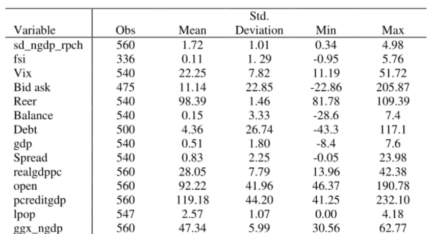
Summary statistics for the bond yield spreads, its main determinants and other macro variables are presented in Table 1.

[Table 1]

In terms of the vector of determinants of yield spreads (VIX, bid ask spread, debt ratio, budget balance ratio, real GDP growth, and REER) in Equation (2), we can postulate the following rational and expected behaviour:

- vix is the logarithm of the S&P 500 implied stock market volatility index (VIX), our proxy

for the international risk factor. The VIX, often called the ‘investor fear gauge’ since it tends to

spike during market turmoil periods (Whaley, 2000), is a reasonable proxy for international financial risk (Mody, 2009) and has been extensively used in the literature on euro area government bond spreads (Beber et al., 2009) and Gerlach et al., 2010). We expect a higher (lower) value for the international risk factor to cause an increase (reduction) in government bond spreads.

- bidask denotes the 10-year government bond bid-ask spread. This is our measure of bond market illiquidity, with a higher (lower) value of this spread indicating a fall (increase) in liquidity leading to an increase (reduction) in government bond yield spreads. Bid-ask spreads are used to capture liquidity effects in the Economic and Monetary Union (EMU) sovereign bond markets by a number of previous studies including Barrios et al. (2009), Favero et al. (2010), Gerlach et al. (2010), and Bernoth and Erdogan (2012).

(9)

8

- reer is the log of the real effective exchange rate. This variable generally captures credit risk originating from general macroeconomic disequilibrium, and may capture external competitiveness. An increase (reduction) in reer denotes real exchange rate appreciation (depreciation), which is expected to increase (reduce) spreads, The empirical significance of real exchange rates in explaining spreads in the EMU area has been confirmed by Arghyrou and Kontonikas (2012).

- gdp is the annual growth rate of GDP (differential versus Germany). This captures the idea according to which sovereign debt becomes riskier during periods of economic slowdown (Alesina et al., 1992, Bernoth et al., 2004). Therefore, an increase (reduction) in growth performance improves (deteriorate) credit worthiness decreasing (increasing) sovereign yield spreads.

4.2. Descriptive statistics and preliminary results

Our main motivation comes from the fact that sovereign bond yield spreads and macroeconomic volatility (proxied by the rolling standard deviation of real GDP growth) are positively correlated, as the stylized evidence shown in Figure 1 for our sample of countries averaged across the 1999-2012 period.

[Figure 1]

Moreover, such increase in yield spread gains special relevance in the aftermath of the

global financial crisis. Using Laeven and Valencia’s (2012) dataset to identify financial crises, we compute the average spread at the time of the beginning of a given crises (for all countries with the exception of Finland, 2008 is a crisis year; Greece also has 2012 as a crisis year) as well as for the quarters immediately before and after. As shown in Figure 2 the yield spreads increase undoubtedly at time “t” and remains persistently high the following quarters.

[Figure 2]

(10)

9

VIX, bid ask, debt-to-GDP ratio or real effective exchange rate positively impact the spreads relative to Germany. These effects are always statistically significant whether one considers them entered individually in a bivariate regression with spreads (columns 1-6) or jointly (column 7). This is the 1st step in our analysis.

[Table 2]

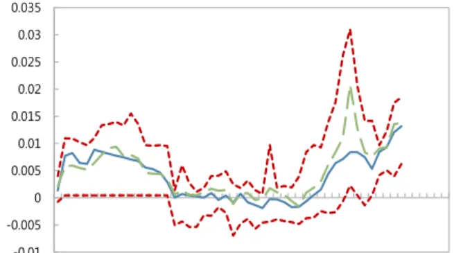
We now take the analysis further, our 2nd step, by estimating the time-varying responses of a given determinant of bond yield spreads. The interquartile time profile of each of the six determinants is displayed in Figure 3. We observe first that the responsiveness of each single determinant increases in absolute value in the run-up to the Global Financial Crisis. Moreover, the amplification effects during the crisis are quite strong and, as already found before, they are clearly yield spread decreasing for rising budged balances and rising growth, and are yield spread increasing for the cases of rising VIX, REER, bid ask spread, and the debt ratio.

[Figure 3]

Looking at the individual country profiles, we notice some relevant patterns concerning the time-varying estimated coefficients. The decreasing yield spread stemming from higher budget balances are more prevalent in Greece, Ireland, Italy, France and Spain. On the other hand, the increase in the debt ratio is related to widening yield spreads mostly in the cases of Greece, France, and Italy. Regarding the decreasing yield spread when there is higher real GDP growth this effect is clearer for the case of Belgium, Italy, and the Netherlands.

Moreover, the other three determinants, where rises go together with increasing yield spreads, reveal more relevance as follows: the bid ask spread, for Austria, Greece, Italy, and Portugal; the REER, for Greece, Ireland, Portugal, Spain, and in more mitigate fashion for Italy; the VIX, for Belgium, Italy, the Netherlands, Spain, and to a lesser extent for Ireland.

(11)

10

4.3. Baseline Regression

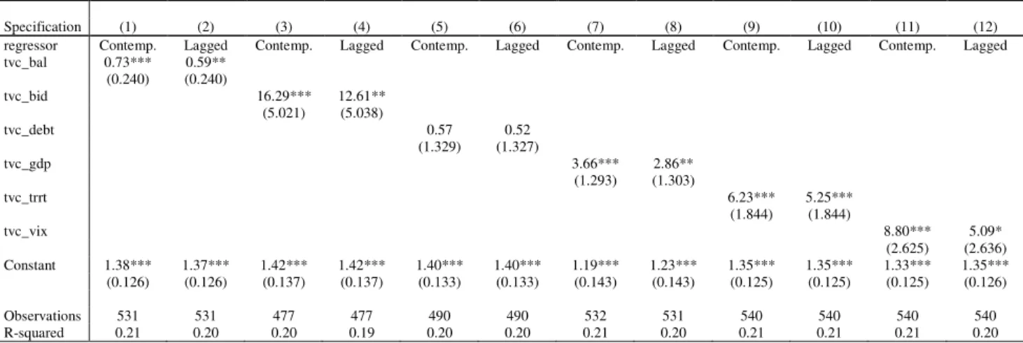
We begin our inspection of the impact of each yield spread’s determinants responsiveness on economic volatility, by estimating equation (4), which is our 3rd step in the analysis. We do so first by including each time-varying coefficient estimate, one at a time, both contemporaneously and lagged.

Results in Table 3 suggest that the for both the budget balance and GDP growth, a decrease in the spread’s responsiveness (recall that both series of time-varying coefficient estimates are negative throughout the time span) or, in other words, the larger in the absolute value the corresponding spread’s responsiveness, the lower the volatility. To put it differently, the faster is the fall in spreads due to an improvement in the budget balance or higher GDP growth expectations (meaning a decrease in the corresponding 𝛽̂_𝑖𝑡), the lower output volatility will be. This can be explained by a higher stabilizing effect of fiscal policy whose positive spillover contributes to smooth overall economic activity. Particularly during the Global Financial Crisis, this means that the continuous downward revision in growth expectations led to rises in yield spreads and this in turn boosted overall economic volatility.

On the other hand, when it comes to the bid ask, the debt-to-GDP ratio, the real effect exchange rate and the VIX, higher spread sensitivities translate directly into higher volatility. For instance, the damaging effect that a rise in the VIX has in the spread relative to Germany, increases output volatility the larger the estimated sensitivity.

[Table 3]

Our baseline results are robust to the use of alternative measures of volatility. More specifically, we replace our dependent variable by the rolling standard deviation of the output gap (computed using the HP filter) and also the Financial Stress Index constructed by Cardarelli et al. (2011) extended to 2012. This can be confirmed in Table 4.

[Table 4]

(12)

11

actually increases, even though the differences are not statistically significant. Among the control variables, we find that trade openness, and credit-to-GDP are positively associated with output volatility. On the other hand, larger and more developed countries as well as those with bigger governments tend to be characterized by lower output volatility.1_{These results are consistent with}

Furceri and Karras (2007), Fatas and Mihov (2001) and Debrun and Kapoor (2010).

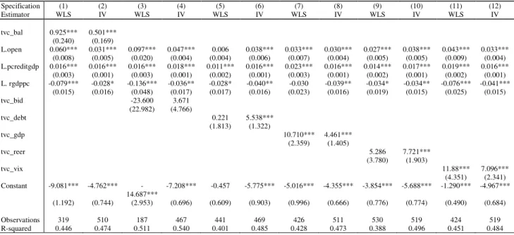
4.4. Robustness

To check the robustness of our results given that our measure of spread determinants’ sensitivities are based on estimates, we re-estimate equation (4) with Weighted Least Squares (WLS), giving more weight to observations that are estimated more precisely. Specifically, the WLS estimator assumes that the errors 𝜖_𝑖𝑡 in equation (2) are distributed as 𝜖_𝑖𝑡~𝑁(0, 𝜎2⁄ )𝑠_𝑖 , where 𝑠𝑖𝑡are the estimated standard deviations of the responsiveness coefficient for each country i, and 𝜎2

is an unknown parameter that is estimated in the second-stage regression. This procedure yields a larger effects on output volatility when the resulting coefficients are statistically different from zero (compare Table 5 and Table 6).

[Table 6]

A concern estimating equation (4) using OLS is that the results may be subject to reverse causality. While in principle this issue is likely to not be relevant in our case, as our measures of

spread’s sensitivities depend on the past, we check the robustness of our results using an IV approach. Following Acemoglu et al. (2003) and Fatas and Mihov (2001, 2013), we select an instrument capturing institutional and political characteristics of the countries that is likely to be correlated with our measures of spread’s responsiveness but presumably not directly related to output volatility. We use the constraints on the executive variable (constraint) as instrument, which captures potential veto points on the decisions of the executive. Another instrument considered is the lag of the respective time-varying sensitivity. As documented by Fatas and Mihov (2013), constraints on the executive are likely to reduce fiscal volatility and therefore reduce overall

1

(13)

12

economic volatility. Results are shown in Table 6 (even columns) and confirm the robustness of our previous findings. In addition, the Kleibergen-Paap test (not shown) confirms the validity of the instruments.

In addition, we complement the IV analysis with a second instrument: the political constraint index produced by Withold Henisz (polcon) that captures not only institutional characteristics in the country, but also political outcomes as its value is adjusted when, for example, the president and the legislature are member of the same party. Results (not shown) are qualitatively similar to the ones when constrain is used as the main instrumental variable.

5. Conclusion

We have studied the link between sovereign bond yield spreads and macroeconomic volatility, two variables that are positively correlated. In practice, we have use a data set for 10 European Union (EU) countries between 1999Q1-2012Q4, and we have implemented a so-called 3-step strategy: first, we assessed the determinants of government bond yield spreads; second, we computed bivariate time-varying coefficient models of each determinant on government bond spreads and collect the resulting estimates; third, we used these estimates as the main explanatory variable of economic volatility.

Our results (step one) show that better fiscal positions (budget balance) or higher than expected GDP growth negatively affect the yield spreads, while increase in the VIX, bid ask spread, debt-to-GDP ratio or real effective exchange rate increase the yield spreads. We also conclude (step two) that the responsiveness of the yield spread determinant increases in absolute value in the run-up to the Global Financial Crisis.

In addition (step three), we observed that for the budget balance and GDP growth, the larger in

the absolute value the corresponding spread’s responsiveness, the lower the volatility. However, for the bid ask spread, the debt-to-GDP ratio, the real effect exchange rate and the VIX, higher spread sensitivities imply higher economic volatility.

(14)

13 References

1. Acemoglu, D., S. Johnson, J. Robinson, and Y. Thaicharoen (2003), “Institutional causes, macroeconomic symptoms: volatility, crises and growth,” Journal of Monetary Economics 50, pp. 49-123.

2. Acharya, V., Drechsler, I., Schnabl, P. (2014). “A Pyrrhic victory? – Bank bailouts and

sovereign credit risk”. Journal of Finance, 69 (6), 2689–2739.

3. Afonso, A. (2010). “Long-term Government Bond Yields and Economic Forecasts:

Evidence for the EU”, Applied Economics Letters, 17 (15), 1437-1441.

4. Afonso, A., Arghyrou, M., Kontonikas, A. (2014). “Pricing sovereign bond risk in the EMU area: an empirical investigation”, International Journal of Finance and Economics, 19 (1), 49–56. 5. Afonso, A., Furceri, D. (2010). “Government size, composition, volatility and economic

growth”, European Journal of Political Economy, 26, 517-532.

6. Afonso, A., Gomes, P., Taamouti, A. (2014). “Sovereign credit ratings, market volatility,

and financial gains”, Computational Statistics and Data Analysis, 76, 20-33.

7. Afonso, A., Rault, C. (2015). “Short and Long-run Behaviour of Long-term Sovereign Bond Yields”, Applied Economics, 47 (37), 3971-3993.

8. Aghion, P. and I. Marinescu (2008), “Cyclical Budgetary Policy and Economic Growth:

What Do We Learn from OECD Panel Data?” NBER Macroeconomics Annual 2007 22: 251–78. 9. Alesina, A., De Broeck, M., Prati, A. and Tabellini, G. (1992), “Default risk on government

debt in OECD countries”. Economic Policy, 15, 427-451.

10. Ardagna, S., Caselli, F., Lane, T. (2004). “Fiscal Discipline and the Cost of Public Debt

Service: Some Estimates for OECD Countries”. EBC Working Paper 411.

11. Arghyrou, M., Kontonikas, A. (2012). “The EMU sovereign debt crisis: Fundamentals,

expectations and contagion”. Journal of International Financial Markets, Institutions and Money, 22, 658-677.

12. Attinasi, M-G., Checherita, C., Nickel, C. (2009). “What explains the surge in euro area sovereign spreads during the financial crisis of 2007-09?”. ECB Working Paper 1131.

13. Barrios, S., Iversen, P., Lewandowska, M., Setzer, R. (2009). “Determinants of

intra-euro-area government bond spreads during the financial crisis”. European Commission, Economic Papers 388.

14. Beber, A., Brandt, M., Kavajecz, K. (2009). “Flight-to-quality or flight-to-liquidity? Evidence from the euro-area bond market”. Review of Financial Studies, 22, 925-957.

15. Bernoth K., J. Von Hagen, L. Schuknecht, (2004), “Sovereign Risk Premia in the European

Government Bond Market”, European Central Bank WP no 369.

16. Bernoth, K., Erdogan, B. (2012). “Sovereign bond yield spreads: A time-varying coefficient

(15)

14

17. Billio, M., Caporin, M. (2010). “Market linkages, variance spillovers, and correlation

stability: Empirical evidence of financial contagion”, Computational Statistics and Data Analysis, 54, 2443-2458.

18. Cardarelli, R., Elekdag, S., Lall, S. (2011). “Financial Stress, Downturns, and Recoveries”,

Journal of Financial Stability, 7 (2), 78-97.

19. Codogno, L., Favero, C., Missale, A. (2003). “Yield spreads on EMU government bonds”.

Economic Policy, 18, 211-235.

20. de Santis, R. (2012). “The euro area sovereign debt crisis: Safe haven, credit rating agencies

and the spread of the fever from Greece, Ireland and Portugal”. ECB Working Paper 1419.

21. Debrun, X., Kapoor, R. (2010), “Fiscal Policy and Macroeconomic Stability: Automatic

Stabilizers Work, Always and Everywhere”, IMF Working Paper/10/111.

22. Elmendorf, D., Mankiw, N. (1999). “Government Debt”, in Taylor, J. and Woodford, M. (eds.), Handbook of Macroeconomics, vol. 1C, 1615-1669, North-Holland.

23. Engle, R., Gallo, G, Velucchi, M. (2012). “Volatility spillovers in East Asian financial markets: a MEM-based approach,” Review of Economics and Statistics, 94(1), 222-223.

24. Fatás, A, Mihov, I. (2013). "Policy Volatility, Institutions, and Economic Growth Policy Volatility, Institutions, and Economic Growth," Review of Economics and Statistics, 95 (2), 362-376.

25. Fatás, A., Mihov, I., (2001). “Government size and automatic stabilizers”, Journal of International Economics, 55, 3-28.

26. Favero, C., Missale, A. (2012). “Sovereign spreads in the euro area. Which prospects for a

eurobond?” Economic Policy, 27 (70), 231-273.

27. Favero, C., Pagano, M., von Thadden, E.-L. (2010). “How does liquidity affect government bond yields?” Journal of Financial and Quantitative Analysis, 45, 107-134.

28. Furceri, D. (2007). Is government expenditure volatility harmful for growth? A cross-country analysis. Fiscal Studies 28(1), 103-120

29. Furceri, D., Karras, G. (2007). "Country size and business cycle volatility: Scale really matters," Journal of the Japanese and International Economies, 21(4), 424-434.

30. Gerlach, S., Schulz, A., Wolff, G. (2010). “Banking and sovereign risk in the Euro area”. CEPR Discussion Paper No. 7833.

31. Geyer, A., Kossmeier, S., Pichler, S. (2004). “Measuring systemic risk in EMU government

yield spreads”. Review of Finance, 8, 171-197.

32. Hui, C., Chung, T. (2011). “Crash risk of the euro in the sovereign debt crisis of

2009-2010”. Journal of Banking and Finance, 35, 2945-2955.

33. Jones, C., Lamont, O., Lumsdaine, R. (1998). “Macroeconomic news and bond market

volatility”, Journal of Financial Economics, 47, 315-337.

(16)

15

35. Lane, Philip R. (2003), “The Cyclicality of Fiscal Policy: Evidence from the OECD,”

Journal of Public Economics 87, 2661-2675

36. Manganelli, S., Wolswijk, G. (2009). “What drives spreads in the euro-area government

bond market?” Economic Policy, 24, 191-240.

37. Mody, A. (2009). “From Bear Sterns to Anglo Irish: How Eurozone sovereign spreads

related to financial sector vulnerability”. IMF Working Paper 09/108.

38. Rodrik, D. (1998). “Who Needs Capital Account Convertibility?”, in Peter Kenen, ed.

“Should the IMF Pursue Capital-Account Convertibility?”. Princeton Essays in International Finance, No. 207.

39. Schlicht, E. (1985), Isolation and Aggregation in Economics, Berlin-Heidelberg-New York-Tokyo: Springer-Verlag.

40. Schlicht, E. (1988), “Variance Estimation in a Random Coefficients Model,” paper presented at the Econometric Society European Meeting Munich 1989, available at http://www.semverteilung.vwl.unimuenchen.de/mitarbeiter/es/paper/schlicht\_variance-estimation-inrandom-coeff-model.pdf

41. Sgherri, S., Zoli, E. (2009). “Euro area sovereign risk during the crisis”. IMF Working Paper 09/222.

42. Talvi, E., Végh,C. (2000). “Tax Base Variability and Procyclical Fiscal Policy,” NBER Working Paper 7499.

(17)

16

Table 1: Summary Statistics

Variable Obs Mean

Std.

Deviation Min Max

sd_ngdp_rpch 560 1.72 1.01 0.34 4.98

fsi 336 0.11 1. 29 -0.95 5.76

Vix 540 22.25 7.82 11.19 51.72

Bid ask 475 11.14 22.85 -22.86 205.87

Reer 540 98.39 1.46 81.78 109.39

Balance 540 0.15 3.33 -28.6 7.4

Debt 500 4.36 26.74 -43.3 117.1

gdp 540 0.51 1.80 -8.4 7.6

Spread 540 0.83 2.25 -0.05 23.98

realgdppc 560 28.05 7.79 13.96 42.38

open 560 92.22 41.96 46.37 190.78

pcreditgdp 560 119.18 44.20 41.25 232.10

lpop 547 2.57 1.07 0.00 4.18

ggx_ngdp 560 47.34 5.99 30.56 62.77

Table 2: Determinants of Yield Spreads

Specification. (1) (2) (3) (4) (5) (6) (7)

balance -0.36*** -0.01

(0.028) (0.010)

bidask 0.03*** 0.02***

(0.001) (0.001)

debt 0.13*** 0.01**

(0.007) (0.003)

gdp -0.89*** -0.12***

(0.041) (0.020)

reer 0.07*** 0.00

(0.021) (0.006)

vix 0.02** 0.01***

(0.012) (0.002) Constant 0.84*** 0.08 -3.27*** 0.80*** -6.09*** -0.10 -0.71

(0.259) (0.063) (0.318) (0.215) (2.089) (0.389) (0.652)

Observations 530 475 490 530 540 540 426

R-squared 0.33 0.70 0.49 0.54 0.14 0.13 0.78

(18)

17

Table 3: Volatility effects of yield spread’s determinants sensitivities – baseline

Specification (1) (2) (3) (4) (5) (6) (7) (8) (9) (10) (11) (12) regressor Contemp. Lagged Contemp. Lagged Contemp. Lagged Contemp. Lagged Contemp. Lagged Contemp. Lagged tvc_bal 0.73*** 0.59**

(0.240) (0.240)

tvc_bid 16.29*** 12.61** (5.021) (5.038)

tvc_debt 0.57 0.52

(1.329) (1.327)

tvc_gdp 3.66*** 2.86**

(1.293) (1.303)

tvc_trrt 6.23*** 5.25***

(1.844) (1.844)

tvc_vix 8.80*** 5.09*

(2.625) (2.636) Constant 1.38*** 1.37*** 1.42*** 1.42*** 1.40*** 1.40*** 1.19*** 1.23*** 1.35*** 1.35*** 1.33*** 1.35*** (0.126) (0.126) (0.137) (0.137) (0.133) (0.133) (0.143) (0.143) (0.125) (0.125) (0.125) (0.126)

Observations 531 531 477 477 490 490 532 531 540 540 540 540 R-squared 0.21 0.20 0.20 0.19 0.20 0.20 0.21 0.20 0.21 0.21 0.21 0.20

Note: tvc – time-varying coefficient. Output volatility measured as the standard deviation of rolling real GDP growth. Results obtained by estimating equation (4). Country and time effects included but omitted for reasons of parsimony. Standard errors in parentheses based on clustered robust standard errors. ***,**,* denote significance at 1,5,10 percent level, respectively.

Table 4: Volatility effects of yield spread’s determinants sensitivities – alternative measures of volatility

Standard Deviation rolling Output Gap Financial Stress Index

Specification (1) (2) (3) (4) (5) (6) (7) (8) (9) (10) (11) (12)

tvc_bal 4.44** 0.24*

(1.764) (0.148)

tvc_bid 29.78*** 6.54**

(7.095) (3.011)

tvc_debt 8.70* 3.66***

(5.044) (0.766)

tvc_gdp 16.77*** 0.34

(4.218) (0.795)

tvc_reer 127.85*** 5.38***

(25.291) (1.120)

tvc_vix 51.69*** -0.24

(11.191) (1.629)

Constant 0.17 0.33* 0.28 -0.47* -0.27 0.22 0.93*** 0.98*** 0.95*** 0.92*** 0.90*** 0.93*** (0.185) (0.181) (0.194) (0.253) (0.202) (0.178) (0.077) (0.082) (0.077) (0.088) (0.076) (0.078)

(19)

18

Table 5: Volatility effects of yield spread’s determinants sensitivities – inclusion of control variables

Specification (1) (2) (3) (4) (5) (6) (7) (8) (9) (10) (11) (12)

tvc_bal 0.610*** 0.455*** (0.146) (0.132)

L.open 0.029*** 0.037*** 0.047*** 0.048*** 0.034*** 0.049*** 0.029*** 0.037*** 0.036*** 0.044*** 0.033*** 0.038*** (0.005) (0.004) (0.004) (0.004) (0.006) (0.004) (0.004) (0.004) (0.005) (0.004) (0.004) (0.004) L.pcreditgdp 0.016*** 0.018*** 0.018*** 0.020*** 0.015*** 0.021*** 0.015*** 0.017*** 0.016*** 0.023*** 0.015*** 0.019***

(0.001) (0.002) (0.001) (0.003) (0.001) (0.003) (0.001) (0.002) (0.001) (0.003) (0.001) (0.002) L.rgdppc -0.028* -0.068*** -0.038** -0.062*** -0.039** -0.096*** -0.042*** -0.076*** -0.034** -0.071*** -0.049*** -0.076***

(0.016) (0.015) (0.017) (0.016) (0.016) (0.015) (0.016) (0.015) (0.015) (0.014) (0.016) (0.015) L.lpop -0.841*** 0.858 -0.645 -1.268*** -3.889* -1.071 (0.139) (2.646) (2.678) (0.137) (2.323) (2.183) L.ggx_ngdp -0.065*** -0.061*** -0.085*** -0.064*** -0.059*** -0.061***

(0.009) (0.010) (0.011) (0.009) (0.009) (0.009) tvc_bid 1.936 6.246*

(3.160) (3.406)

tvc_debt 4.125*** 5.918***

(1.126) (1.207)

tvc_gdp 4.678*** 2.671**

(1.044) (1.076)

tvc_reer 7.359*** 8.084***

(1.853) (2.123)

tvc_vix 9.594*** 4.996**

(2.044) (2.396) Constant -4.387*** -4.441*** -7.249*** -6.344 -5.110*** -2.001 -4.022*** -5.316*** -5.375*** 4.957 -4.779*** -0.408 (0.690) (0.801) (0.696) (5.928) (0.850) (6.091) (0.625) (0.813) (0.762) (5.174) (0.653) (4.846)

(20)

19

Table 6: Volatility effects of yield spread’s determinants sensitivities – robustness to alternative estimators

Specification (1) (2) (3) (4) (5) (6) (7) (8) (9) (10) (11) (12) Estimator WLS IV WLS IV WLS IV WLS IV WLS IV WLS IV

tvc_bal 0.925*** 0.501*** (0.240) (0.169)

L.open 0.060*** 0.031*** 0.097*** 0.047*** 0.006 0.038*** 0.033*** 0.030*** 0.027*** 0.038*** 0.043*** 0.033*** (0.008) (0.005) (0.020) (0.004) (0.004) (0.006) (0.007) (0.004) (0.005) (0.005) (0.009) (0.004) L.pcreditgdp 0.016*** 0.016*** 0.016*** 0.018*** 0.011*** 0.016*** 0.023*** 0.016*** 0.014*** 0.017*** 0.019*** 0.016***

(0.003) (0.001) (0.003) (0.001) (0.002) (0.001) (0.003) (0.001) (0.002) (0.001) (0.002) (0.001) L. rgdppc -0.079*** -0.028* -0.136*** -0.036** -0.028* -0.040** -0.030 -0.039** -0.034* -0.034** -0.076*** -0.041***

(0.015) (0.016) (0.048) (0.017) (0.017) (0.016) (0.023) (0.016) (0.019) (0.015) (0.025) (0.015) tvc_bid -23.600 3.671

(22.982) (4.766)

tvc_debt 0.221 5.538***

(1.813) (1.322)

tvc_gdp 10.710*** 4.461***

(2.359) (1.405)

tvc_reer 5.286 7.721***

(3.780) (1.903)

tvc_vix 11.88*** 7.096***

(4.351) (2.341) Constant -9.081*** -4.762***

-14.687***

-7.208*** -0.457 -5.775*** -5.016*** -4.355*** -3.854*** -5.688*** -1.290*** -4.967***

(1.192) (0.744) (2.953) (0.696) (0.609) (0.903) (0.996) (0.666) (0.776) (0.774) (0.490) (0.684)

(21)

Figure 1: Spreads and Volatility in 10 EU countries, average 1999Q1-2012Q4

Figure 2: Spreads before and after Global Financial Crisis

Note: the horizontal axis represents quarters before and after the financial crisis. “t” denotes the beginning quarter of the financial crisis.

belgium austria finland

france

greece

ireland

italy netherlands

portugal

spain

y = 0,4077x + 1,4748 R² = 0,348

0,75 1,25 1,75 2,25 2,75 3,25

-0,25 0,25 0,75 1,25 1,75 2,25 2,75 3,25

0 0.2 0.4 0.6 0.8 1 1.2 1.4 1.6 1.8

(22)

21

Figure 3: Interquartile Time Profile of spread’s determinants responsiveness, 1999-2012

Balance Bid Ask

Debt GDP

REER VIX

-0.8 -0.7 -0.6 -0.5 -0.4 -0.3 -0.2 -0.1 0 0.1

1999Q1 2000Q3 2002Q1 2003Q3 2005Q1 2006Q3 2008Q1 2009Q3 2011Q1

median pctile_75 pctile_25 mean

-0.01 -0.005 0 0.005 0.01 0.015 0.02 0.025 0.03 0.035 1999Q12000Q32002Q12003Q32005Q12006Q32008Q12009Q32011Q1

-0.04 -0.02 0 0.02 0.04 0.06 0.08 0.1 0.12 0.14 1999Q12000Q32002Q12003Q32005Q12006Q32008Q12009Q32011Q1

-0.2 -0.18 -0.16 -0.14 -0.12 -0.1 -0.08 -0.06 -0.04 -0.02 0 1999Q12000Q32002Q12003Q32005Q12006Q32008Q12009Q32011Q1

-0.02 -0.01 0 0.01 0.02 0.03 0.04 0.05 0.06 0.07 0.08 0.09 1999Q12000Q32002Q12003Q32005Q12006Q32008Q12009Q32011Q1

-0.02 -0.01 0 0.01 0.02 0.03 0.04 0.05 0.06 0.07 1999Q12000Q32002Q12003Q32005Q12006Q32008Q12009Q32011Q1

(23)

22

Figure 4: Country-specific

-2 -1 .5 -1 -.5 0 -2 -1 .5 -1 -.5 0 -2 -1 .5 -1 -.5 0 -2 -1 .5 -1 -.5 0 -2 -1 .5 -1 -.5 0 -2 -1 .5 -1 -.5 0 -2 -1 .5 -1 -.5 0 -2 -1 .5 -1 -.5 0 -2 -1 .5 -1 -.5 0 -2 -1 .5 -1 -.5 0

0 20 40 60 0 20 40 60

Belgium austria finland france

greece ireland italy netherlands

portugal spain

tvc_bal group(time)

Graphs by country

TVC-Spreads on Balance

-.0 5 0 .0 5 .1 -.0 5 0 .0 5 .1 -.0 5 0 .0 5 .1 -.0 5 0 .0 5 .1 -.0 5 0 .0 5 .1 -.0 5 0 .0 5 .1 -.0 5 0 .0 5 .1 -.0 5 0 .0 5 .1 -.0 5 0 .0 5 .1 -.0 5 0 .0 5 .1

0 20 40 60 0 20 40 60

portugal spain

tvc_bid group(time)

Graphs by country

TVC-Spreads on Bid Ask

-.1 0 .1 .2 .3 -.1 0 .1 .2 .3 -.1 0 .1 .2 .3 -.1 0 .1 .2 .3 -.1 0 .1 .2 .3 -.1 0 .1 .2 .3 -.1 0 .1 .2 .3 -.1 0 .1 .2 .3 -.1 0 .1 .2 .3 -.1 0 .1 .2 .3

0 20 40 60 0 20 40 60

portugal spain

tvc_debt group(time)

Graphs by country

TVC-Spreads on Debt

-.3 -.2 -.1 0 .1 -.3 -.2 -.1 0 .1 -.3 -.2 -.1 0 .1 -.3 -.2 -.1 0 .1 -.3 -.2 -.1 0 .1 -.3 -.2 -.1 0 .1 -.3 -.2 -.1 0 .1 -.3 -.2 -.1 0 .1 -.3 -.2 -.1 0 .1 -.3 -.2 -.1 0 .1

0 20 40 60 0 20 40 60

portugal spain

tvc_gdp group(time)

Graphs by country

TVC-Spreads on GDP

-.1 0 .1 .2 -.1 0 .1 .2 -.1 0 .1 .2 -.1 0 .1 .2 -.1 0 .1 .2 -.1 0 .1 .2 -.1 0 .1 .2 -.1 0 .1 .2 -.1 0 .1 .2 -.1 0 .1 .2

0 20 40 60 0 20 40 60

portugal spain

tvc_reer group(time)

Graphs by country

TVC-Spreads on REER

0 .0 5 .1 .1 5 0 .0 5 .1 .1 5 0 .0 5 .1 .1 5 0 .0 5 .1 .1 5 0 .0 5 .1 .1 5 0 .0 5 .1 .1 5 0 .0 5 .1 .1 5 0 .0 5 .1 .1 5 0 .0 5 .1 .1 5 0 .0 5 .1 .1 5

0 20 40 60 0 20 40 60

portugal spain

tvc_vix group(time)

Graphs by country

(24)

23 Table A1: Data definition and sources

Variable Description Source

Spread 10 year government bond yield (differential vs. Germany) ECB/Reuters Vix (Log of) S&P 500 implied stock market volatility index (VIX) Bloomberg

Bid ask 10 year government bond bid-ask spread ECB

REER (Log of) CPI based real effective exchange rate IMF Balance Expected budget balance/GDP (differential vs. Germany) European

Commission Debt Expected debt/GDP (differential vs. Germany) European

Commission GDP GDP annual growth (differential vs. Germany) IMF

Trade openness Exports plus imports over GDP IMF

Financial development

Domestic credit to the private sector (percent of GDP) World Bank WDI

Real GDP per capita

GDP at constant 2005 USD divided by population IMF

Population Population in millions World Bank WDI

Government size

Total public expenditure (percent of GDP) IMF