(Annals of the Brazilian Academy of Sciences)
Printed version ISSN 0001-3765 / Online version ISSN 1678-2690 http://dx.doi.org/10.1590/0001-3765201820170829
www.scielo.br/aabc | www.fb.com/aabcjournal
The phase portrait of the Hamiltonian system associated to a Pinchuk map
JOAN CARLES ARTÉS1, FRANCISCO BRAUN2and JAUME LLIBRE3
1,3Departament de Matemàtiques, Universitat Autònoma de Barcelona, Edifici Cc, Campus de la UAB, Bellaterra, Cerdanyola del Vallès, 08193 Barcelona, Catalonia, Spain
2Departamento de Matemática, Universidade Federal de São Carlos, Rodovia Washington Luís, Km 235, Caixa Postal 676, 13565-905 São Carlos, SP, Brazil
Manuscript received on October 22, 2017; accepted for publication on December 13, 2017
ABSTRACT
In this paper we describe the global phase portrait of the Hamiltonian system associated to a Pinchuk map in the Poincaré disc. In particular, we prove that this phase portrait has 15 separatrices, five of them singular points, and 7 canonical regions, six of them of type strip and one annular.
Key words:center, global injectivity, real Jacobian conjecture, Pinchuk map.
INTRODUCTION
As far as we know, the simplest class of non-injective polynomial local diffeomorphisms of R2 are the Pinchuk maps, constructed by Pinchuk (1994). The existence of these maps disproves thereal Jacobian conjecture, that a polynomial local diffeomorphism of R2 is globally injective. One open problem is to know what exactly fails in this conjecture.
One of the most known conditions for a local diffeomorphism to be a global one is that it is proper. The asymptotic variety of a map ofR2 is the set of points where the map is not proper (i.e., points that are limits of the map under sequences tending to infinity). In particular, a local diffeomorphism is a global diffeomorphism if and only if this set is empty. Gwoździewicz (2000) and Campbell (arXiv:math/9812032 in 1998, 2011) calculated the asymptotic variety of two Pinchuk maps in details. Our aim in this paper is to do a similar work, i.e., to describe a Pinchuk map, but now from a different point of view.
LetU⊂R2be an open connected set. LetF= (p,q):U⊂R2→R2be aC2local diffeomorphism. Let HF(x,y) = (p(x,y)2+q(x,y)2)/2and consider the Hamiltonian system
˙
x=−(HF)y(x,y), y˙= (HF)x(x,y), (1)
where the dot denotes derivative with respect to the timet. The singular points of system (1) are characterized by the following result, that we shall prove below.
Lemma 1. The singular points of system(1)are the zeros ofF, each of them is a center of system(1). The following is a generalization of the characterization of global invertibility of polynomial maps given by Sabatini (1998). This version is due to Braun and Llibre (arXiv:1706.02643 in 2017).
Theorem 2. Letz0∈Usuch thatF(z0) = (0,0). The centerz0of system(1)is global if and only if (i)F is globally injective and (ii)F(U) =R2orF(U)is an open disc centered at the origin.
In the special case thatF is a polynomial map andU =R2, it follows thatF(R2) =R2providedF is injective (Białynicki-Birula and Rosenlicht 1962). Hence, in this case,z0is a global center of (1) if and only
ifF is globally injective. An application of this result was given by Braun et al. (2016).
Since the phase portrait on the Poincaré sphere of a Hamiltonian polynomial vector field having a global center is simple, i.e., at the infinite either it does not have singular points, or the infinite singular points are formed by two degenerate hyperbolic sectors (for Hamiltonian vector fields, the infinity contains only isolated singular points), it is interesting to know how complex can be the phase portrait of a non-global center of a Hamiltonian system (1).
In this paper we provide the qualitative global phase portrait of the Hamiltonian system (1) whenF is given by the Pinchuk map considered by Campbell (1998, 2011), after a translation in the target in order to have only a pointz0such thatF(z0) = (0,0). More precisely, we prove the following result.
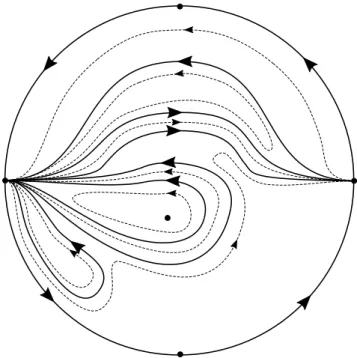
Theorem 3. Let F= (p,q):R2 →R2, where(p,q+208):R2→R2 is the Pinchuk map considered by Campbell (1998, 2011) (see the definition below). Then the phase portrait of the Hamiltonian system(1)in the Poincaré disc is topologically equivalent to the phase portrait given in Fig. 1.
Figure 1 -The qualitative global phase portrait of system (1) in the Poincaré disc.
Then, we complete the proof of Theorem 3 by proving that the separatrix configuration of system (1) is qualitatively the one presented in Fig. 1.
We think that a good understanding of what fails in the real Jacobian conjecture could be interesting to investigate a related problem, theJacobian conjectureinR2, that a polynomial local diffeomorphism whose
Jacobian determinant is constant is globally injective. This conjecture remains unsolved until now. For the Jacobian conjecture we address the reader to the works of Bass et al. (1982) and Van Den Essen (2000).
INJECTIVITY, CENTERS AND A PINCHUK MAP
We begin with the proof of Lemma 1.
Proof of Lemma 1. Letz0be a singular point of the Hamiltonian system (1). We have
−py(z0) −qy(z0)
px(z0) qx(z0)
p(z0)
q(z0)
= 0 0 ,
which is true if and only inF(z0) = (p,q)(z0) = (0,0)because the Jacobian determinant ofF is nowhere
zero.
The pointz0is a center of the Hamiltonian system (1) because it is an isolated minimum ofHF.
Now, we select the mapF that we are going to work in this paper. Lett=xy−1,h=t(xt+1)and f= (xt+1)2(t2+y). APinchuk mapis a non-injective polynomial map with nowhere zero Jacobian determinant
of the form(P,Q):R2→R2such thatP=h+f andQ=−t2−6th(h+1)−u(h,f), whereuis chosen so
thatdetD(P,Q)(x,y) =t2+ (t+f(13+15h))2+f2. The following is the Pinchuk map studied by Campbell (1998, 2011):
p=h+f,
q=−t2−6th(h+1)−170f h−91h2−195f h2−69h3−75f h3−75h 4
4 .
According to Campbell (2011), the points(−1,−163/4)and(0,0)∈R2have no inverse image under (p,q), all the other points of the curve
γ(s) =
s2−1,−75s5+345s
4
4 −29s
3+117s2
2 − 163
4
, s∈R,
which is a parametrization of the asymptotic variety of(p,q), have exactly one inverse image under this map, and the points ofR2\γ(R)have two inverse images. Hence, in particular, the point(0,208)has precisely
one inverse image under(p,q).
We consider the mapF= (p,q):R2→R2given by the translation
Observe thatFis a Pinchuk map according to our above-definition. Moreover, now there exists exactly one pointz0∈R2such thatF(z0) = (0,0). From Lemma 1 the pointz0is the only finite singular point of system
(1), corresponding to a non-global center of this system according to Theorem 2. Further, the curve
β(s) =γ(s)−(0,208) =
s2−1,−75s5+345s
4
4 −29s
3+117s2
2 − 995
4
, (3)
s∈R, is the asymptotic variety ofF, whose points have exactly one inverse image overF, but the points (−1,−995/4)and(0,208), which have none.
From now on, we restrict our attention to the specific Pinchuk map (2).
We first calculate the coordinates of the pointz0. Observe thatxt+1=x2y−x+1is a factor of p. If
this factor annihilates, thenh=0andq=−t2−208<0. The other factor ofpis
g(x,y) =−x+ (1−2x+3x2)y−x2(−2+3x)y2+x4y3.
We observe thatg(0,y) =y and q(0,y) =50y−799/4 do not annihilate at the same time, thus the first coordinate of the pointz0is not0. Moreover, since the leading coefficient ofq(x,y)as a polynomial inyis −75x15, it follows that the first coordinate ofz0will be a point where the resultant inybetweeng(x,y)and
q(x,y)is zero. This resultant is the cubicc(x) =31008391−11757152x−155580672x2+2239078400x3 multiplied by−x36/64. The discriminant ofc(x)is negative, so it has only one real root, which will be the first coordinate of the pointz0.
Repeating a similar reasoning now looking g and q as polynomials in x, we calculate their resul-tant and obtain that its zero is the only real root of the cubicc(y) =1789023641600+100675956992y+ 26252413280y2+1506138481y3, which will be the second coordinate of the pointz0.
Hencez0= (−0,22568337...,−17,491214...)approximately. Sincez0is a center, the only finite
sin-gular point of system (1), nearz0the phase portrait of this system is simple. Indeed, sincez0is the minimum
point ofHF, it follows that the gradient ofHF points outward of each closed orbit of the center, and so each
closed orbit of the center rotates in counterclockwise aroundz0.
In the following section we shall investigate the infinite of system (1).
THE INFINITE OF SYSTEM
In this section, we will use results and notations on thePoincaré compactification of polynomial vector fields ofR2. In particularUi,Vi,i=1,2,3, are the canonical local charts of the Poincaré sphereS2.
For details on this technique we refer the reader to Chapter 5 of (Dumortier et al. 2006) or to (González Velasco 1969).
We call a singular point of a vector fieldlinearly zerowhen the linear part of the vector field at this point is identically zero.
We begin by proving a general fact about the infinite singular points of Hamiltonian systems of the form (1). WritingH=H0+H1+· · ·+Hd+1, whereHiis the homogeneous part of degreeiof the polynomialH,
the points satisfyingHd+1(1,u) =0andHd+1(u,1) =0, respectively. Let(u,0)be an infinite singular point
of system (1) and assume it is in the chartU1. The linear part of the vector field at(u,0)is
(d+1)(Hd+1)y(1,u) dHd(1,u)
0 (Hd+1)y(1,u)
.
Assumingm=degp≥degq, we haved=2m−1andHd=pmpm−1+qmqm−1andHd+1=p2m+q2m. Since
Hd+1(1,u) =0, it follows thatpm(1,u) =qm(1,u) =0, and hence(Hd+1)y(1,u) =Hd(1,u) =0. Therefore,
(u,0)is a linearly zero singular point. This proves the following result.
Lemma 4. The infinite singular points of the Hamiltonian system(1)are linearly zero.
Now, we return to the Pinchuk mapF defined by (2). Observe that the highest homogeneous part of HF(x,y)is5625x30y20/2. Thus, the origins of the chartsU1,V1andU2,V2are the infinite singular points of
the Hamiltonian system (1), each of them linearly zero from Lemma 4.
We will use the quasi-homogeneous directional blow up technique to desingularize each of these infinite singular points. An exposition about blow-ups can be found in (Álvarez et al. 2011), see also Chapter 3 of (Dumortier et al. 2006). We now recall the directional blow up transformations.
By thequasi-homogeneous blow up in the positive(resp.negative)x-direction with weightsαandβ, or
simply(α,β)-blow up in the positive(resp.negative)x-direction, we mean the transformation which carries the variables(x1,y1)to the variables(x2,y2)according to the formulas
(x1,y1) = (xα2,x β
2y2), (x1,y1) = (−xα2,x β 2y2),
respectively. Similarly, by thequasi-homogeneous blow up in the positive(resp.negative)y-direction with
weights α and β, or simply (α,β)-blow up in the positive (resp. negative) y-direction, we mean the transformations
(x1,y1) = (x2yα2,y β
2), (x1,y1) = (x2yα2,−y β 2),
respectively.
Clearly ifα (resp.β) is odd, then, the blow up in the positivex-direction (respec.y-direction) provides
the information of the respectively negative blow ups. Also, ifβis odd, thex-directional blow ups swap the
second and third quadrants, while they-directional blow ups swap the third and the fourth quadrants ifα is
odd. After the(α,β)-blow up in thex-direction, a systemx˙1=P(x1,y1),y˙1=Q(x1,y1)is transformed into
˙ x2=
±P
αxα2−1, y˙2=
αxα2−1Q∓βxβ2−1y2P αxα+β2 −1
,
with P=P(±x2α,xβ2y2) and Q=Q(±xα2,xβ2y2), in the positive and negative directions according to ±.
Similarly, the(α,β)-blow up in they-direction transformsx˙1=P(x1,y1),y˙1=Q(x1,y1)into
˙ x2=
βyβ2−1P∓αx2yα2−1Q βyα+β2 −1
, y˙2= ±Q
βyβ2−1
withP=P(x2yα2,±yβ2)andQ=Q(x2yα2,±yβ2), in the positive and in the negative directions according to ±.
After the blow up in thex-direction (resp.y-direction) we cancel a common appearing factorxk2(yk2) for a suitablek. So, ifkis odd, the direction of the orbits are reversed inx2<0(y2<0).
The weights α and β are chosen analyzing the Newton polygon of (P,Q), see the construction in (Álvarez et al. 2011).
The application of(α,β)-blow ups withαβ6=1usually reduces the number of blow ups necessary for studying the local phase portrait of a linearly zero singular point.
To make the exposition clearer, we shall apply the most part of the blow ups in thex-direction. So, sometimes, we will first apply axy-change,(x1,y1)7→(y1,x1) = (x2,y2), before making the blow-up.
In the next two subsections we will desingularize the origin of the chartsU1andU2, respectively. We
will denote the coordinates of the system in the stepiof the algorithm as the variables(wi,zi), so that after
either a wz-change, a translation or a blow up, the new obtained system will be written in the variables (wi+1,zi+1). In each step, we will denote the systemw˙i=Pi(wi,zi),z˙i=Qi(wi,zi)simply as(Pi,Qi).
Since the Hamiltonian system (1) with the polynomials pandqgiven by (2) has degree49, it follows that for the calculations in each step of the algorithm we have to deal with polynomials of very high degree. So, we persuade these calculations with the algebraic manipulatorMathematica. We do not show in each step the whole expressions of the systems(Pi,Qi)because this would be impractical.
THE ORIGIN OF THE CHARTU1
We write the compactification of system (1) in the chartU1 in the variables (w0,z0), as(P0,Q0). From
Lemma 4, the singular point(0,0)is linearly zero.
We first apply awz-change and write the new system in the variables(w1,z1)as(P1,Q1).
The Newton polygon of system(P1,Q1)has only one compact edge contained in the straight linex+
2y=38. We apply(1,2)-blow ups in the positivew-direction and in the positive and negativez-directions obtaining systems(P2,Q2)and(P2±,Q±2), in the variables(w2,z2)and(w±2,z±2), after canceling the common
factorsw382 and(w±2)38, respectively. The first terms of these systems have the following expressions:
P2=w2
−56250+1125
2 (447w2+1900z2) +· · ·
,
Q2=28125−
1125
4 (387w2+2000z2) + 75
4 (1967w
2
2+24138w2z2+57000z22) +· · ·,
and
P2±=w±2
∓28125
2 +281250(w
±
2) 2+· · ·
,
Q±2 =z±2
±140625
2 −1350000(w
±
2) 2+· · ·
.
The only singular point of(P2,Q2) over the linew2=0is the linearly zero singular point(0,1). The
origin of the systems(P2±,Q±2)are saddles as depicted in the planesw+2z+2 andw−2z−2 of Fig. 2.
wz-change wz-change
translation
α= 1,β= 2
α= 1,β= 2
α=β= 1
α=β= 1
z-dir w-dir
w-dir
w-dir odd odd
even
even
w0 z0
w1 z1
w2 z2
w3 z3
w4 z4
w5 z5
w6 z6
w− 2 z−
2
w+ 2 z+
2
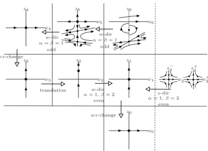
Figure 2 -The sequence of blow downs in the study of the origin of the chartU1.
We now analyze this linearly zero singularity. We first do a translation bringing this point to the origin, obtaining the new system(P3,Q3)in the variables(w3,z3). We also apply awz-change obtaining the system
(P4,Q4)in the variables(w4,z4). The Newton polygon of this system has two compact edges. We choose the
one contained in the straight linex+y=11. This compact edge has the point of negative abscissa(−1,12), thus, concerning(1,1)-blow ups, it follows from Proposition 3.2 of (Álvarez et al. 2011) thatw4 is not a
characteristic direction, and so we only need to apply aw-directional(1,1)-blow up, obtaining the system (P5,Q5)in the variables(w5,z5), after canceling the common factorw115 . The first terms of(P5,Q5)are:
P5=w5
1
4(w5+z5)(w5+2z5) 442125w
5
5z5+824250w45z25+699990w35z 3 5
+320532w25z45+215904w5z55+112500w65+217160z65
+· · ·,
Q5=z5
1
4(w5+z5)(w5+2z5) 442125w
5
5z5+824250w45z25+699990w35z35
+320532w25z45+215904w5z55+112500w65+217160z65
+· · ·.
(4)
Over the linew5=0, the singular points of(P5,Q5)are(0,0)and two points of the form(0,z5), withz5the
two real solutions of
0=z45+70726z35+252941z25+290380z5+108580.
The discriminant of this quartic equation is negative, thus, it has two real solutions. Those are approximately z5=−70722.424...andz5 =−1.6611121.... The singular point (0,0) is linearly zero and the other two
singular points are saddles, as represented in thew5z5-plane of Fig. 2.
Now, we study the linearly zero point(0,0)of(P5,Q5). It is clear from (4) that the characteristic equation
of(P5,Q5)is identically zero, so(0,0)is a dicritical singular point. We apply(1,1)-blow ups in both the
the factorsw96and(zy6)9, respectively. System(Py
6,Q
y
6)does not have(0,0) as a singular point, so we just
need to consider system(P6,Q6)over the linew6=0. We have
P6(0,z6) =
1
4(z6+1)(2z6+1) 217160z
6
6+215904z56+320532z46+699990z36
+824250z26+442125z6+112500
,
Q6(0,z6) =
1 4z
2
6(z6+1)(2z6+1) 290380z66+260416z56+421348z46+904140z36
+1032225z26+542250z6+135000
.
By using Sturm’s theorem (see for instance (Isaacson and Keller 1994); in the software Mathematica, the Sturm theorem is programed by the instructionCountRoots) we see that the polynomial of degree 6 mul-tiplying (z6+1)(2z6+1)/4in P6(0,z6) has no real roots, so, the only singular points are(0,−1/2) and
(0,−1). The first one is a weak focus and the second one is a saddle, as depicted in the planew6z6of Fig. 2.
Since the origin of(P5,Q5)is dicritical, it follows that each orbit crossing the linew6=0will correspond
to two orbits tending to(0,0)in positive or negative directions. We now begin the process of blowing down.
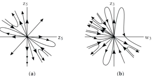
It is simple to conclude that the phase portrait of the system(P5,Q5)close to the origin is qualitatively
the one depicted in (a) of Fig. 3. Consequently, by considering also the information close to the other two
z5
z5
(a)
w3
z3
(b)
Figure 3 -The origin of system(P5,Q5)in (a) and the origin of system(P3,Q3)in (b).
singular points in the linew5=0(see the planew5z5 of Fig. 2), we can understand the behavior near the
origin of system(P4,Q4). We then apply awz-change and conclude that the behavior of system(P3,Q3)near
the origin is the one presented qualitatively in (b) of Fig. 3.
By translating(0,0)to(0,1)and by using the information provided by the saddles of planesw±2z±2, we make the blow downs withα=1andβ =2, obtaining the origin of system(P1,Q1). We then finally apply
awz-change and conclude that the origin of system(P0,Q0)is qualitatively as drawn in Fig. 4.
w0 z0
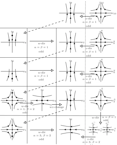
THE ORIGIN OF CHARTU2
As in the calculations made above, we write the compactified vector field in the chartU2 as(w˙0,z˙0) =
(P0,Q0). The Newton polygon of(P0,Q0)has two compact edges: one of them contained in the straight line
3x+2y=87. We apply a(3,2)-blow up in thew-direction, obtaining the system(w˙1,z˙1) = (P1,Q1)after
canceling the factorw871 . The first terms ofP1andQ1are:
P1=w1 −46875+11250z21(80w1−47z1) +· · ·
,
Q1=z1 9375+56250z12(2z1−3w1) +· · ·
.
The polynomialsP1andQ1have degree61.
It is clear that at(0,0)we have a saddle. The other singular point of(P1,Q1)in the linew1=0is(0,−1),
and it is a linearly zero point. See thew1z1-plane of Fig. 5. The reader can follow the steps of the calculations
in the schema shown in this figure. We just warn that, differently of Fig. 2, we already draw the final phase portrait of each step, including the behavior close to the linearly zero points (information that we will know only after persuading all the blow ups).
wz-change
α=β= 1
α= 3,β= 2
α= 3,β= 2
α= 1,β= 2
α=β= 1
α=β= 1
α=β= 1
α=β= 1
α=β= 1
z-dir z-dir z-dir z-dir w-dir w-dir w-dir w-dir w-dir odd odd odd odd odd odd odd odd odd w0 z0 w1 z1 w2 z2 w3 z3 w4 z4 w5 z5 w6 z6 wy 6 zy 6 w7 z7 w8 z8 wy 8 zy 8 w9 z9 w10 z10 w− 1 z− 1 w+ 1 z+ 1 w± 2 z ± 2
We also apply(3,2)-blow ups in the positive and negativez-directions, obtaining the systemsw˙±1 =P1±, ˙
z±1 =Q±1, respectively, with linearly zero singular points at(w±1,z±1) = (0,0). The polynomialsP1± andQ±1 have degree30andQ±1 is a factor ofz±1.
We do not need to analyze the other singular points over the linesz±1 =0, as the information provided by them is already contained in thew-directional blow up. We desingularize these points applying(1,1)-blow ups in thew-direction. Here, we do not need to apply blow ups in thez-directions because the characteristic equations of the systems are
0=z±1 −4500(w±1)5z±
1 +1650(w±1)4(z±1)2−7800(w±1)3(z±1)3
+3025(w±1)2(z1±)4−500w±1(z±1)5+5625(w±1)6+2501(z±1)6,
and sow±1 =0 are not characteristic directions. We obtain the systems(P2±,Q±2) after canceling a factor (w±2)5. The polynomialsP±
2 andQ±2 have degree45, and up to order2they have the same expressions:
P2±=w±2
−28125
2 +10125z
±
2 +· · ·
,
Q±2 =z±2 5625−4500z±2 +· · · .
Thus, at (0,0) the systems have a saddle, as depicted in the planesw±2z±2 of Fig. 5. Moreover, any other singularity of the form(0,z±2)must satisfy
2501(z±2)6−500(z±2)5+3025(z±2)4−7800(z±2)3+1650(z±2)2−4500z±2 +5625=0.
By using Sturm’s theorem, we conclude that this equation has no real solution.
Now, we desingularize the point(0,−1)of system(P1,Q1). First, we apply a translation to bring this
point to the origin, obtaining the system(P2,Q2)in the variables(w2,z2). We also apply awz-change
obtain-ing the system(P3,Q3)in the variables(w3,z3). The Newton polygon of this system has only one compact
edge contained in the linex+2y=11, and this edge has points of negative abscissa, so, concerning(1,2) -blow ups we just need to apply them in thew-direction, according to Proposition 3.2 of (Álvarez et al. 2011). Hence, we apply a(1,2)-blow up in the positivew-direction, obtaining the system(P4,Q4)in the variables
(w4,z4), after canceling a factor ofw114 . These polynomials have degree90, and their first terms are:
P4=w4
−4982259375+996451875
4 (260w4+z4) +· · ·
,
Q4=z4(3985807500−110716875(639w4+2z4) +· · ·).
Clearly,(0,0)is a singularity corresponding to a saddle. The other singular point in the linew4=0is(0,ξ),
whereξ is the only real root of the cubic
c(x) =4x3+216x2+6075x−218700,
which is approximately ξ =18.8848... This cubic has only one real root because its discriminant is
negative. A calculation shows that(0,ξ)is linearly zero. See the planew4z4in Fig. 5.
Now, we apply a translation to bring the point(0,ξ) to the origin, obtaining system(P5,Q5)written
thusP5 andQ5 are polynomials inw5, z5 andx. We simplify these polynomials substituting them by the
remainder of the division of each of them byc(x), obtaining so polynomials of degree 2inx, and hence when we substitutexbyξ, we obtain the same expressions. We keep the notation(P5,Q5).
The Newton polygon of this system has just one compact edge contained in the linex+y=1. So, the blow ups here will be homogeneous ones. The characteristic equation of system(P5,Q5)is a multiple of
0=w5 729 23090824x2+532204875x−18375684300
w25
−216 149x2+1828125x−32221800w5z5−4 404x2+8325x−54675
z25,
withx=ξ. It would thus be enough to apply a(1,1)-blow up in thez-direction, and to study the singularities of the new system inz6=0(this could evidently also be concluded by observing that the compact edge of
the Newton polygon of(P5,Q5)has a point of negative ordinate). We prefer though to apply(1,1)-blow ups
in thewandz-directions and to study the singularities of the new systems either in the linew6=0and in the
origin, respectively. The reason why we do this is that the singularities other than the origin are linearly zero and we have to apply new blow ups after persuading a translation. The matter here is that the blow up in thez-direction produces a vector field of degree158, while the blow up in thew-direction produces a vector field of degree109. Thus, it is simpler to do a translation and after to apply the polynomial remainder in the vector field with smaller degree.
Then, after applying (1,1)-blow ups in either the positivew- andz-directions, we obtain the systems (P6,Q6)and(P6y,Qy6)in the variables(w6,z6)and(wy6,zy6), after canceling factorsw6 andzy6, respectively.
The first terms of these systems are:
P6=w6
59049 4 149x
2+1828125x−32221800
+· · ·
,
Q6=−
4782969
16 23090824x
2+532204875x−18375684300
+177147
64 5928191012x
2−9644385686625x+179165168144100
w6
+177147 2 149x
2+1828125x−32221800
z6+· · ·,
withx=ξ and
P6y=wy6
−6561
4 (404x
2+8325x−54675) +· · ·
,
Qy6=zy6 2187(404x2+8325x−54675) +· · · ,
withx=ξ.
The origin of system (P6y,Qy6) is a saddle (see the plane wy6zy6 in Fig. 5). On the other hand, the singularities of(P6,Q6)over the linew6=0are the points(0,z6), withz6the real solutions of
0=4 404x2+8325x−54675z62+216 149x2+1828125x−32221800z6
−729 23090824x2+532204875x−18375684300, (5)
coefficients ofz26andz6in (5), respectively. Substitutingx byξ after applying the polynomial remainder
again we have
r1=
3 2380ξ2+21ξ−334440
5989
The point(0,r1)is linearly zero, so, we translate it to the origin obtaining the system(P7,Q7)in the variables
(w7,z7). We again persuade this translation consideringr1=r1(x)as a polynomial ofx. AgainP7andQ7will
be polynomials inw7,z7andx. As before we substitute these polynomials by the remainder of the division
of them byc(x), obtaining polynomials of degree2inx. We keep the notationP7andQ7for them.
The Newton polygon of this system has only one compact edge contained in the straight linex+y=1. The characteristic equation of this system hasw7=0as a solution.
As above, we apply (1,1)-blow ups in either the positive w- andz-directions, obtaining the systems (P8,Q8)and(P8y,Q
y
8)in the variables(w8,z8)and(wy8,z
y
8), respectively. We then study the origin of(P
y
8,Q
y
8)
and the singularities of(P8,Q8)over the linew8=0. The reason is again computational, as the degree of
(P8y,Qy8)is196and the degree of(P8,Q8)is128. The first terms of these systems are:
P8=w8 −
6561 610023097091x2−7154910819000x−72219849901200
95824 +· · ·
!
,
Q8=
59049
4591119488 866106385697199684752x
2−63678825997496319079125x
+894244583851567110026100+· · ·,
withx=ξ, and
P8y=w8
−2187
2 (404x
2+8325x−54675) +· · ·
,
Qy8=z8
6561 4 (404x
2+8325x−54675) +· · ·
,
withx=ξ.
System(P8y,Qy8)has a saddle at the origin (see the planewy8zy8 in Fig. 5), while the singular points of (P8,Q8)over the linew8=0are the points(0,z8), withz8the real roots of
0=2295559744 404x2+8325x−54675z28−574944 610023097091x2
−7154910819000x−72219849901200z8+27 866106385697199684752x2
−63678825997496319079125x+894244583851567110026100,
withx=ξ. The discriminant of this equation is a polynomial inxwhose division byc(x)has remainder0. Thus, the only real solution isr2=−b/(2a), whereaandbare the coefficients ofz28andz8of the equation,
respectively. After applying the polynomial remainder, we substitutexbyξ obtaining
r2=
−38570325688ξ2−1361034154573ξ+41691943772820
430417452 .
The point(0,r2)is linearly zero, so, we translate it to the origin obtaining the system(P9,Q9)in the variables
(w9,z9). As before, we make this translation with the parameterx, so thatP9 andQ9are polynomials inx.
As before the Newton polygon of this system has only one compact edge contained in the straight line x+y=1. Moreover, the characteristic equation does not have z9 =0 as a solution. Here, we just apply
a (1,1)-blow up in the positive z-direction, obtaining system (P10,Q10) in the variables (w10,z10), after
canceling the factorz10 (here we do not use the superscripty as this is the only system in this step). The
degree of this new system is234, but as we are going to see, just the origin is a singular point in the line z10=0. The first terms ofP10andQ10 are:
P10=w10
−2187
4 (404x
2+8325x−54675) +· · ·
,
Q10=z10
2187 2 (404x
2+8325x−54675) +· · ·
,
withx=ξ.
Now, over the linez10=0, the singular points of(P10,Q10)are(0,0)and the points(w10,0), withw10
the real roots of
0=27(224799605593831132981000196646508x2
+11060763183198622719418769173796625x
−289048399074933337876985160926408100)w210
−1721669808(375535867201456283x2+10785776535503894250x
−338993606077717260600)w10+41168707330260512(404x2+8325x−54675),
withx=ξ. The discriminant of this equation after applying the polynomial remainder is
∆(x) =42795139080321190650757595864867731660278486158784x2 +2546081344010178238089386481604981090589087283168000x
−63345629158853164845226783632142224359340633182668800.
It is simple to conclude that∆(ξ)<0, thus, only(0,0) is a singular point of (P10,Q10) inz10=0. This
singular point is the saddle depicted in the planew10z10of Fig. 5.
Since the behavior near each appearing singular points in each step above is very simple, the blow down of each step is also very simple: following the arrays in Fig. 5, it is easy to conclude that the origin ofU2
has a degenerate hyperbolic sector as shown in thew0z0-plane of Fig. 5.
THE GLOBAL PHASE PORTRAIT
We begin with a background on separatrices and canonical regions of the Poincaré compactificationp(X)
in the Poincaré discDof a polynomial systemx˙=X(x). Letϕbe the flow ofp(X)defined inD. As usual we denote by(U,ϕ)the flow ofp(X)on an invariant subsetU⊂D. Two flows(U,ϕ)and(V,ψ)are said to betopologically equivalent if there exists a homeomorphismh:U →V sending orbits of(U,ϕ) onto orbits of(V,ψ)preserving or reversing the orientation of all the orbits.
the system in polar coordinatesr˙=r,θ˙ =0. Parallel flows topologically equivalent to (i), (ii) and (iii) are calledstrip,annularandspiral(orradial), respectively.
We denote by γx the orbit of p(X) passing throughx whent=0with maximal intervalIx, and the
positive (resp. negative) orbit ofγxbyγx+={γx(t)|t∈Ixandt≥0}(resp.γx−={γx(t)|t∈Ixandt≤0}).
Then we seta±(x) =γx±\γx±, here as usualγx± denotes the closure ofγx±. Observe thata−(x)differs from
α(x)in the case of periodic orbits and singular points: indeed,a−(x) =/0andα(x) =γxin this case (similarly
fora+(x)andω(x)). An orbitγx ofp(X)is called aseparatrixofp(X)if it is not contained in an open
neighborhoodUsuch that(U,ϕ)is parallel and such that botha±(x) =a±(y)for ally∈UandU\Uconsists ofa+(x),a−(x)and exactly two orbitsγyandγzsuch thata±(x) =a±(y) =a±(z).
IfX is a polynomial vector field it is known that the separatrices ofp(X)are (i) the finite and infinite
singular points ofp(X); (ii) the orbits ofp(X)contained in the boundaryS1ofD; (iii) the limit cycles of p(X); and (iv) the separatrices of the hyperbolic sectors of the finite and infinite singular points ofp(X).
Moreover, if p(X)has finitely many finite and infinite singular points and finitely many limit cycles, then
p(X)has finitely many separatrices. We call each connected component of the complement of the union
of separatrices acanonical regionofp(X). Neumann (1975) proved that each canonical region of a vector
field p(X)is parallel.
To the union of the separatrices of p(X) together with an orbit belonging to each canonical region
of p(X)we call aseparatrix configurationofp(X). We say that the separatrix configurationsS1andS2
ofp(X1)andp(X2)aretopologically equivalentif there exists an orientation preserving homeomorphism
fromDtoDwhich transforms orbits ofS1onto orbits ofS2. The following is the Markus-Neumann-Peixoto classification theorem (Markus 1954, Neumann 1975, Neumann and O’Brien 1976, Peixoto 1973, Dumortier et al. 2006) for the Poincaré compactification in the Poincaré disc of polynomial systems.
Theorem 5(Markus-Neumann-Peixoto). Let p(X1)and p(X2)be the Poincaré compactification of two
polynomial systemsx˙=X1(x)andx˙=X2(x), respectively. The flows ofp(X1)andp(X2)on the Poincaré
disc are topological equivalent if and only if the separatrix configurations of p(X1) and p(X2) are
topological equivalent.
Hence, in order to qualitatively describe the phase portrait on the Poincaré disc of system (1) it is enough to qualitatively describe its separatrix configuration. This was done in Fig. 1, where we have drawn the separatrices other than singular points with bold lines. The other lines are orbits contained in its respective canonical regions. We observe from Fig. 1 that system (1) has15separatrices, five of them singular points, and7canonical regions, six of them of type strip and the one formed by the closed orbits surroundingz0,
annular.
Below, we prove Theorem 3 by proving that Fig. 1 is a separatrix configuration of system (1).
From the previous sections we conclude that close enough to the singular points, the phase portrait of system (1) is qualitatively the one presented in Fig. 6. For further references we label the hyperbolic, parabolic and elliptic sectors presenting in the origins of the chartsU1andV1in Fig. 6 ash1,h2,h3,h4, p1,
p2ande1,e2, respectively.
From the definition of system (1), each of its orbits is a connected component of a level set ofHF =
(p2+q2)/2(because the only singular point of this system is the center z0), which in turn is the inverse
h1
h2
p1
p2
h3
h4
e1
e2
Figure 6 -The phase portrait of system (1) near the singular points.
counterclockwise orientation. As we have seen, the curveβ(s)defined in (3) is the asymptotic variety ofF. Moreover, the pointsβ(0) = (−1,−995/4)andβ(1) = (0,208)of this curve have no inverse image under F, all the other points of this curve have exactly one inverse image and the other points ofR2have precisely two inverse images. Acting as Campbell (arXiv:math/9812032 1998), we delete from the curveβ(s) the pointsβ(0)andβ(1), obtaining three curves:C1=β(−∞,0),C2=β(0,1)andC3=β(1,∞). According to
Campbell (1998), the inverse image underFof eachCiis a curve that divides the plane into two connected
components. We callDithe inverse image ofCi,i=1,2,3. The setD1∪D2∪D3is called by Campbell (1998)
theasymptotic flowerofF. It follows thatR2\(D1∪D2∪D3)is formed by4connected components, each of them mapped twice onto each of the two connected components ofR2\ {β(s)}. Each curveCi has a natural orientation, given by its parametrization (it is the opposite orientation used by Campbell (1998)). So, each curveDi also has a natural orientation (recall thatFpreserves orientation). The graphics ofCiand
Di,i=1,2,3, are given in (a) and (b) of Fig. 7, respectively. As in (Campbell 1998, 2011) the axes in (a)
have different scales. Following Campbell (1998), we label the regions asR(right) andL(left) of the curves Ci andDi.
−1 − 1
1 2
1 2
−300
300
−150
150
C1
C2 C
3 L
R R
(a)
D1
D2
D3 L
L
R
R
(b)
Since for eachs∈R
β′(s)·β(s) =1
4(1−s)s(s+1) 112500s
6−232875s5+301125s4−425760s3
+432312s2−86565s+116423,
and this polynomial of degree6multiplying(1−s)s(s+1)has no real zeros by Sturm’s theorem, it follows that the curvesC1,C2andC3are transversal to the circles centered at(0,0) =β(−1). As a consequence the
curvesD1,D2andD3 are transversal to the non-singular orbits of system (1). In particular, the image of a
non-periodic orbit of system (1) hasα- andω-limits contained in the curveβ(s). Below, we will say that the image of an orbitstartsorfinishesatβ(s0)meaning that itsα- orω-limit isβ(s0), respectively. Moreover,
through each point in the intersection ofC1∪C2∪C3with a circle, it crosses exactly one image of an orbit
of system (1).
We callS1andS2the circles centered at(0,0)and containing the pointsβ(1)andβ(0), respectively.
The pointz0, being the inverse image under F of(0,0) =β(−1), is contained in the curveD1. The
images underF of the closed orbits surroundingz0are circles surrounding(0,0)contained in the bounded
region defined by S1. Thus the boundary of the period annulus of the centerz0 corresponds to the arc of
circle contained inS1, starting and finishing at the pointβ(1). This means that the boundary of the period
annulus is an orbit that goes to infinity through the region labeled byLin (b) of Fig. 7. In particular, in the Poincaré disc, this orbit tends to the origin of the chartV1. Then, analyzing the possibilities in Fig. 6, we see
that this orbit contains the two separatrices of the hyperbolic sectorh2. This period annulus is an annular
canonical region.
Now we analyze the parabolic sectorsp1andp2.
Close to the two points ofD1cut by the orbit giving the boundary of the period annulus of the center (i.e.,
the orbit connecting the two separatrices of the hyperbolic sectorh2), and outside the period annulus, there
must exist orbits cuttingD1. Analyzing the images of these orbits, they are contained in circles surrounding
the circleS1. So, there are two possibilities for the images of these orbits: either they are arcs starting and
finishing at a point of the curveC2, or they are arcs starting at the curveC3and finishing at the curveC2or
C3. At a first glance both of these possibilities are compatible with the parabolic sectorsp1 and p2in Fig.
6. Weclaim that the correct possibility is the first one. Indeed, we can increase the radii of these circles containing the images of the orbits of p1 and p2 until we achieve the circleS2. If we are in the second
possibility, the orbit whose image is contained inS2and starts at a point ofC3will contain the separatrice of
the end of the parabolic sector p2. But, this orbit will not contain the separatrice of the end of the parabolic
sector p1, because we can continue drawing arcs starting atC3with radii bigger than the radius ofS2. Thus,
the parabolic sectorp1will not finish, a contradiction with the nature of the vector field at the origin of the
chartV1, as shown in Fig. 6. This proves the claim.
So, the image of the orbits of the parabolic sectorsp1 andp2are arcs starting and finishing at a point
of the curveC2. And since we can continue drawing these arcs until we arrive at circleS2, this means that
the parabolic sectors p1 and p2 are connected, and the image of the orbit containing the separatrices that
separatep1fromh1andp2fromh3is contained in the arc ofS2starting and finishing at the pointβ(0). The
region connecting p1top2is a strip canonical region, see Fig. 1.
Now, since the image of this last orbit cuts the curvesC3andC1, there must exist orbits near it whose
rotating a complete turn crossingC3andC1and continue up to finishing in the curveC3. We call these orbits
thebig orbits. A big orbit whose image is contained in a circle close enough toS2enters both the hyperbolic
sectorsh1andh3. We have to see where the big orbits start and finish.
The orbits whose images are arcs of the circles with radii smaller than the radius ofS2, starting and
finishing atC1 and contained in the regionRcorrespond to an elliptic sector with boundary formed by an
orbit having image contained in the arc ofS2starting atC1an finishing atβ(0). Close to this boundary and
out of the elliptic sector there must exist orbits whose images start atC1. These orbits are the big orbits.
Hence, it follows that this elliptic sector ise1and that the big orbits start at the origin ofV1, see Fig. 1.
The orbits whose images are arcs starting and finishing atC1and contained in the regionLform the
elliptic sectore2. Clearly its boundary is formed by the two orbits containing the separatrices of the
hyper-bolic sectorh4. The image of these orbits are the arcs starting atC1and finishing atβ(1)and starting atβ(1)
and finishing atC1, respectively.
In particular, this means that the big orbits must finish at the origin of the chartU1, below the hyperbolic
sectorh4. Since their images are contained in the circles bigger thanS2, there exist orbits whose images are
arcs contained in the circles betweenS1andS2, starting atC1, crossingC2and finishing atC3. These orbits
produce a parabolic sector betweenh3ande2, and give rise to a strip canonical region as presented in Fig. 1.
The big orbits also produce a strip canonical region.
The orbits of the strip canonical region placed above the hyperbolic sector h4 have their images
contained in arcs of circles with radii bigger than the radius ofS1, starting atC3and finishing atC1.
The elliptic sectorse1ande2form another two strip canonical regions.
Hence we have 7 canonical regions, six of them are strip and one is annular. Analyzing Fig. 1, we see there are6finite orbits that are separatrices. The infinite has another4orbits. Hence, since there are5 singular points, we have15separatrices in the separatrix configuration of system (1) in the Poincaré disc.
ACKNOWLEDGMENTS
The first and third authors are partially supported by the Ministerio de Economia y Competitividad (MINECO) grant number MTM2013-40998-P, the Agència de Gestió d’Ajuts Universitaris i de Recerca (AGAUR) grant number 2014SGR 568 and the grants from European Commission (FP7-PEOPLE-2012-IRSES) numbers 316338 and 318999. The second author is partially supported by Fundação de Amparo à Pesquisa do Estado de São Paulo (FAPESP), grant number 2014/ 26149-3. The second and third authors are also partially supported by Coordenação de Aperfeiçoamento de Pessoal de Nível Superior (CAPES), grant 88881. 030454/ 2013-01 from the program CSF-PVE.
REFERENCES
ÁLVAREZ MJ, FERRAGUT A AND JARQUE X. 2011. A survey on the blow up technique. Internat J Bifur Chaos Appl Sci Engrg 21: 3103-3118.
BASS H, CONNEL EH AND WRIGHT D. 1982. The Jacobian conjecture: reduction of degree and formal expansion of the inverse. Bull Amer Math Soc 7: 287-330.
BIAŁYNICKI-BIRULA A AND ROSENLICHT M. 1962. Injective morphisms of real algebraic varieties. Proc Amer Math Soc 13: 200-203.
BRAUN F, GINÉ J AND LLIBRE J. 2016. A sufficient condition in order that the real Jacobian conjecture inR2holds. J Differential
Equations 260: 5250-5258.
DUMORTIER F, LLIBRE J AND ARTÉS JC. 2006. Qualitative theory of planar differential systems. Universitext, Springer-Verlag, 298 p.
GONZÁLEZ VELASCO EA. 1969. Generic properties of polynomial vector fields at infinity. Trans Amer Math Soc 143: 201-222. GWOŹDZIEWICZ J. 2000. A geometry of Pinchuk’s map. Bull Polish Acad Sci Math 48: 69-75.
ISAACSON E AND KELLER HB. 1994. Analysis of numerical methods, Corrected reprint of the 1966 original Wiley. New York: Dover Publications, 541 p.
MARKUS L. 1954. Global structure of ordinary differential equations in the plane. Trans Amer Math Soc 76: 127-148. NEUMANN DA. 1975. Classification of continuous flows on2-manifolds. Proc Amer Math Soc 48: 73-81.
NEUMANN DA AND O’BRIEN T. 1976. Global structure of continuous flows on2-manifolds. J Differ Equations 22: 89-110.
PEIXOTO MM. 1973. On the classification of flows on2-manifolds. Dynamical systems (Proc. Sympos., Univ. Bahia, Salvador,
1971). New York: Academic Press, p. 389-419.
PINCHUK S. 1994. A counterexample to the strong real Jacobian conjecture. Math Z 217: 1-4.
SABATINI M. 1998. A connection between isochronous Hamiltonian centres and the Jacobian conjecture. Nonlinear Anal 34: 829-838.