Comparing covariance matrices: Random skewers method compared to the common principal components model

Comparing covariance matrices: Random skewers method compared

to the common principal components model

James M. Cheverud

and Gabriel Marroig

1

Department of Anatomy and Neurobiology, Washington University School of Medicine, Saint Louis,

MO, USA.

2

_{Departamento de Genética e Biologia Evolutiva, Instituto de Biociências, Universidade de São Paulo,}

São Paulo, SP, Brazil.

Abstract

Comparisons of covariance patterns are becoming more common as interest in the evolution of relationships be-tween traits and in the evolutionary phenotypic diversification of clades have grown. We present parallel analyses of covariance matrix similarity for cranial traits in 14 New World Monkey genera using the Random Skewers (RS), T-statistics, and Common Principal Components (CPC) approaches. We find that the CPC approach is very powerful in that with adequate sample sizes, it can be used to detect significant differences in matrix structure, even between matrices that are virtually identical in their evolutionary properties, as indicated by the RS results. We suggest that in many instances the assumption that population covariance matrices are identical be rejected out of hand. The more interesting and relevant question is, How similar are two covariance matrices with respect to their predicted evolu-tionary responses? This issue is addressed by the random skewers method described here.

Key words:covariance matrix, common principal components, random skewers, New World monkeys, quantitative genetics.

Received: July 11, 2006; Accepted: January 31, 2007.

Introduction

The evolution of phenotypic and genetic variance/ covariance matrices, referred to as simply covariance ma-trices throughout this paper, is a crucial subject in evolu-tionary biology (Steppanet al.2002). In a pivotal paper Lande (1979) showed that, under certain assumptions, esti-mation of the additive genetic variance-covariance matrix (G) enables us to predict how a set of quantitative traits will evolve under conjoint operation of mutation and genetic drift or in response to natural selection (Lande and Arnold 1983; Turelli 1988). The pattern and level of additive inher-itance described byG-matrices is also crucial to the “evolu-tionary constraints” approach, which seeks to understand the existing diversity of life forms from comparisons of pat-terns of phenotypic, and ideally genetic, interrelationships among continuous distributed traits (Cheverud 1984, 1996; Steppan 1997; Arnold and Phillips 1999). Both, phenotypic (P) and genetic (G) matrices are important for understand-ing the evolution of complex morphologies for several rea-sons. First, genetic correlations and variance/covariance

parameters are estimated from phenotypic attributes, prop-erly weighted by genealogical information. Second, al-though theGmatrix helps determine the rate and direction of evolutionary response to natural selection, phenotypic covariance patterns give us direct information about the pattern and level of variation available for selection and are the ultimate target of selection. Phenotypic matrices also play a role in the multivariate evolutionary response equa-tion for natural selecequa-tion

(Δz= Gβ)

because the gradient selection vectorβ, which summarizes the directional selection force operating on each individual character independently of other traits, is calculated as the inverse of the phenotypic matrix times the selection differ-ential (S) (β= P-1S), whereΔz is the evolutionary change in a vector of trait means. Third, there is increasing evi-dence that phenotypic and genetic variance/covariance ma-trices are quite similar, especially for morphological traits, in many diverse organisms (Cheverud 1988, 1995, 1996; Roff 1995, 1996; Steppan 1997; Waitt and Levin 1998; Ar-nold and Phillips 1999; Marroig and Cheverud 2001), al-lowing P matrices to be substituted for G matrices in evolutionary studies.

Send correspondence to James M. Cheverud. Department of Anat-omy and Neurobiology, Washington University School of Medicine, 660 S. Euclid Ave., Campus Box 8108, Saint Louis, MO, 63110, USA. E-mail: cheverud@pcg.wustl.edu.

pendent on reliable statistical methods, a research area that has been growing during the last two decades. Several methods have been proposed and used for comparing covariance and correlation matrices (Lovsfold 1986; Shaw

et al., 1995; Cheverud 1988, 1995, 1996), from vector cor-relation among principal components to matrix corcor-relation and a maximum-likelihood test for matrix equality. Re-cently, Roff and colleagues (Begin and Roff 2001, 2003, 2004; Roff 2002; Beginet al.2004) have introduced a se-ries of new matrix comparison methods, including the T-method, an element by element approach, using percent reduction in Mean Square Error, and the Jackknife-MANOVA method. The T-method (Roffet al. 1999) in-volves the calculation of the overall sum of the absolute values of differences between the elements of two symmet-rical matrices, in other words:

T A_ij B_ij

j n

i n

= −

= =

∑

∑

where Aijis the covariance between traits i and j in matrix A

and Bij is the corresponding covariance in matrix B, the

summation being extended to all diagonal and off diagonal elements in the two matrices (sum of the number of diago-nal elements plus the number above or below the diagodiago-nal). Similarly, T2statistics can be calculated which are basically the sum of the squared differences between corresponding matrix elements (instead of the module). Both statistics can be extended to three or more populations by computing all pairwise comparisons. To test the null hypothesis that the elements in one matrix from one population do not differ from the corresponding elements in the other population matrix, we estimate the probability associated with each T value observed via randomizations. Hypothesis testing is conducted by permuting individuals between data arrays and calculating pseudovalues of T or T2from the random-ization procedure (Trand T2r). Significance is evaluated as

the fraction of times Tobs> Tr(or T2obs> T2r). Steppanet al.

(2002) have recently reviewed many of these methods. Common principal component analysis (CPC) has been suggested as a potentially useful tool for simulta-neously comparing covariance matrices among two or more taxa (Flury 1988; Steppan 1997; Phillips and Arnold 1999; Arnold and Phillips 1999). CPC analysis is particu-larly well suited for covariance matrix comparisons be-cause it allows a diversity of hypotheses of relationships among matrices (from unrelated structure to proportional-ity and equalproportional-ity) to be tested in a hierarchical fashion using any number of matrices (Flury 1988; Phillips and Arnold 1999; Arnold and Phillips 1999). This analysis is based on the description and comparisons of matrices using their de-composition into eigenvalues and eigenvectors (principal components). Flury’s model (1988) allows covariance ma-trices to share more complex relationships than just being

common principal components) besides matrix equality or unrelated structure (Phillips and Arnold 1999). In this way, CPC analysis builds and tests a hierarchy of relationships among two or more covariance matrices, from unrelated structure to PCPC1, sharing the first PC, PCPC2, sharing the first two PCs,and so on until CPC, sharing all PCs, pro-portionality and finally equality, each step up in the hierar-chy being more inclusive and only being true if the lower levels also holds (see Phillips and Arnold 1999). For each hypothesis in the hierarchy a new set of matrices based on the sample (original) matrices is constructed by maxi-mum-likelihood methods that are constrained so that the hypothesis in question is true. The relative degree of differ-ence between the original and constrained matrices deter-mines the likelihood that the particular hypothesis is true. The difference between the likelihood function values of two steps in the hierarchy is distributed as a chi-square and therefore a standardχ2

test could be used to detect signifi-cant differences in matrix structure. The CPC test does not have an associated parameter designating the strength of similarity among matrices, relying only on significance testing. We propose a metric described below based on the extent of shared PC structure.

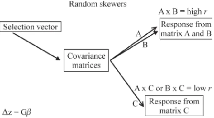
comparisons will differ depending on the specific multi-variate dimension tested, so we use the average vector cor-relation between matrix responses to as many as 10,000 random selection vectors as an overall measure of matrix similarity. If two matrices are equal, the average response to random selection vectors is expected to be co-linear or equals one and contrarily, if two matrices are completely unrelated with no shared structure, the average response is expected to be perpendicular or equal to zero (Figure 1).

The statistical significance of a random skewers set can be evaluated against the null hypothesis of no shared structure by using the distribution of vector correlations among ‘k’ element random, unit-length vectors, where ‘k’ is the number of traits in the analysis. If the observed vector correlation exceeds 95% of the vector correlations found among the random vectors, there is significant structural similarity between the covariance matrices. In practice, the null hypothesis of no structural similarity is nearly always rejected. Alternatively, a bootstrap approach can be used to measure variation in matrices drawn from population sam-ples. Cheverudet al.(1989; Cheverud, 1996) used a boot-strap test of self-matrix correlation to evaluate matrix re-peatability. A bootstrap sample of N individuals is produced by randomly sampling N individuals, with re-placement, from the population. A covariance matrix is generated from this sample and compared to the original observed covariance matrix using the random skewers pro-cedure. Covariance matrix repeatability is given by the av-erage squared vector correlation between predicted selec-tion responses of the observed and bootstrap matrices. This approach can also be used to test the null hypothesis of no difference between two covariance matrices by comparing the bootstrap sample matrices from one species with the ob-served covariance matrix of the other species (see below).

This paper has three goals: first, present a distribution free method for comparing pairs of covariance matrices based on the expected similarity among responses to ran-dom selection vectors; second, evaluate these results in re-lation to Roff’s T-test; third, discuss some possible

problems in interpreting results from the CPC analysis associated with sample sizes of the matrices compared, problems that one should be aware of in order for the full potential of CPC as a tool in evolutionary studies to be real-ized.

Materials and Methods

Thirty-nine skull measurements were taken on 5,222 Neotropical primate specimens deposited in several natural history museums (a complete list of material with specimen numbers, museum and taxonomy used can be obtained upon request from the authors). This data set is the same as used by Marroig and Cheverud (2001). Of the sixteen Platyrrhine (Strepserrhini, Primates) genera, two (BrachytelesandCallimico) were excluded because their small sample sizes preclude the proper application of the CPC program (Phillips 1998). Pooled within-groups phenotypic variance/covariance matrices were obtained for each genus following procedures outlined in Marroig and Cheverud (2001) by correcting for sex and taxonomic vari-ation within genus (specific or sub-specific rank depending on the taxonomic arrangement employed for each genus).

Both, T- and T2statistics (Roffet al.1999) were ap-plied to test whether or not each pair of NWM covariance matrices were statistically different. The software to imple-ment both T- statistics was kindly provided by L.J. Revell (http://iguana.wustl.edu/~liam/programs/index.htm). Be-cause the T-method relies on bootstrapping the data, recal-culating each covariance matrix in every step of the 1,000 samplings, specimen values should be used as a input for the program, not the covariance matrices. Because nearly all of our matrices are pooled-within groups matrices al-ready accounting for other sources of variation (such as sex, species, or sex by species interaction), we used the residu-als of the appropriate general linear model for each genus as the data input for the T-method. Variance/ covariance ma-trices were also analyzed using the CPC software (Phillips 1998) in a pairwise fashion for each possible combination of the 14 South American primate genera. We use both the step-up and the model building approaches (Arnold and Phillips 1999; Phillips and Arnold 1999) to interpret CPC results. The number of partial common principal compo-nents analyzed was limited to seven, since for this data set few loadings beyond the fifth principal component are sig-nificantly different from zero. The results from CPC analy-ses were transformed into scores in order to be able to correlate those results with the harmonic or geometric mean of the sample sizes of the matrices involved in each comparison. The full CPC hierarchy comprises 10 catego-ries, from unrelated structure to equality and therefore equality was considered as one and unrelated as zero. Any result between these extreme possibilities was considered as a proportion of the total number of categories. For exam-ple, if two matrices had 7 principal components in com-mon, the similarity between those 2 matrices is 0.7

“similarity matrix”, this matrix was correlated with the ma-trix of harmonic and geometric means of the sample sizes using matrix correlation and the Mantel’s test. The signifi-cance of the observed matrix correlation was calculated us-ing 10,000 permutations of the columns and associated rows and by comparing the observed matrix correlation to the distribution of randomized matrix correlations.

Phillips and Arnold (1999) suggested that when con-sidering CPC results and differences in the results among the approaches used to build the CPC hierarchy (Step-up, Jump-up and Model-Building approaches) the biological reality of the situation can be gleaned by looking at how well the matrices constructed using the constrained model match the actual matrices from the populations. Therefore, we select four cases to further examine the possible influ-ence of the sample sizes upon the CPC results. These four cases correspond to the following situations: full CPC re-sult with low average sample size; full CPC rere-sult with high average sample size; unrelated structure with high average sample size; and unrelated structure with low average sam-ple size. For each of these four examsam-ples the original matri-ces were compared to several reconstructed matrimatri-ces con-strained by the PCPC or CPC models, from PCPC1 to proportionality. The comparisons were made using the Random Skewers procedure with the VCVCOMP pro-gram, which is available from the authors upon request. Al-though matrix correlation followed by Mantel’s test be-tween paired matrices has been used for comparing variance/covariance matrices matrix (Lovsfold 1986; Ar-nold and Phillips 1999) this approach is not suitable for comparing this kind of matrix. Columns and rows of vari-ance/covariance matrices usually differ in scale because larger measurements tend to have larger variances and the reverse is true for smaller measurements. This scaling prob-lem means that the randomized columns and associated rows of the variance/covariance matrix are not strictly com-parable to one another.

The Random Skewers (RS) procedure does not have this scale problem because the columns and rows of both matrices are not randomized. Instead, the randomization is obtained by repeatedly varying the selection vector applied to both matrices in each round. We compare the same 14 variance/covariance matrices used in the T-method and CPC analyses using the RS method (for a complete analy-ses of this data set see Marroig and Cheverud 2001). The re-sulting similarity matrix among the 14 Neotropical primate genera was also compared to CPC results and sample sizes using matrix correlation followed by Mantel’s test. In order to better understand the properties of the RS method, we use a Monte Carlo approach to look at pairwise similarity between any two matrices. Since samples used to estimate pooled-within groups covariance matrices have a structure, which controls for variation associated with sex and

taxo-mdata sets, each composed ofnindividuals with 39 mea-surements randomly drawn from a population having the observed covariance structure, wherenstands for the num-ber of specimens in the original sample. This is performed using the Cholesky decomposition. The covariance matrix specified by each of thesemdata sets is calculated and then compared to the observed matrix of the other genus in-volved in the pairwise comparison using the average vector correlation between simulated selection responses. In this way, the distribution of correlations around the observed random skewer can be observed.

Results

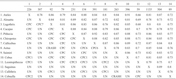
Table 1 presents the CPC results for each pairwise comparison among the 14 New World Monkey generic covariance matrices and their sample sizes. Table 1 also presents the Random Skewers results above the diagonal. There is a negative and significant correlation between the CPC results transformed to a similarity matrix and both the harmonic (r = -0.374, p = 0.0065) and geometric means (r = -0.410, p = 0.0012) of the sample sizes. This indicates that increasing the average sample sizes of the matrices de-creases the apparent similarity of the matrices. It is more difficult to reject the hypothesis of common structure with smaller samples. This is reinforced by the comparison of the observed matrices of the four selected cases (with com-binations of high or low sample sizes and unrelated or CPC structure) to the matrices constructed using the constrained models of the CPC hierarchy (Table 2). All pairwise com-parisons show high similarity between the reconstructed matrices and the original ones at all levels in Flury’s hierar-chy, except for a few matrices in theCacajaoxCebuella

if the same two matrices (CallithrixandSaguinus) are com-pared again using the CPC, but using a 10 times smaller sample size as input, the result for all 3 approaches indicate a full proportional relationship between them.

There is a low, non-significant correlation between RS results and CPC results (r = 0.163, p = 0.18) indicating that the techniques are giving different answers to the ques-tion of matrix similarity. This is because RS uses a quanti-tative measure of association, not based on sample sizes, while CPC results are largely determined, in our data set, by sample size considerations. There is also a positive and sig-nificant correlation between the RS results and both,

har-monic mean (r = 0.453, p = 0.0198) and geometric mean (r = 0.413, p = 0.0286) of the matrix sample sizes. This re-sult indicates that matrices with higher sample sizes appear to be more similar than matrices with lower sample sizes. This probably results from the fact that matrices with high sample sizes are estimated with more confidence than ma-trices with lower sample sizes. Note that this is in opposi-tion to the associaopposi-tion between CPC interpretaopposi-tions and sample sizes.

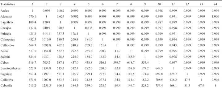
Tables 4 and 5 present the results of the T- and T2 -sta-tistics, with observed values below the diagonal and associ-ated probabilities above the diagonal. Notice that among all

Table 1- CPC results between each pairwise comparison of the fourteen Neotropical primate covariance matrices shown below the diagonal. Comparisons are rated as equal (EQ), proportional (PROP), sharing all principal components (CPC), sharing the first X principal components (CPCX), and unrelated (UN). The Random Skewers results are presented above the diagonal. Sample sizes are shown in the second row.

1 2 3 4 5 6 7 8 9 10 11 12 13 14

226 387 92 79 231 154 391 181 263 396 59 1135 504 89

1. Ateles X 0.78 0.86 0.79 0.84 0.88 0.84 0.8 0.84 0.91 0.66 0.81 0.87 0.72

2. Alouatta UN X 0.84 0.81 0.89 0.82 0.87 0.72 0.82 0.81 0.69 0.78 0.73 0.72

3. Lagothrix CPC CPC7 X 0.81 0.86 0.83 0.86 0.76 0.82 0.85 0.68 0.8 0.8 0.75

4. Cacajao CPC UN CPC X 0.88 0.84 0.88 0.79 0.86 0.83 0.7 0.79 0.78 0.72

5. Pithecia UN UN CPC CPC X 0.87 0.92 0.83 0.87 0.88 0.73 0.86 0.83 0.77

6. Chiropotes CPC UN CPC CPC CPC X 0.88 0.82 0.85 0.88 0.71 0.84 0.85 0.75

7. Callicebus UN UN UN CPC UN UN X 0.87 0.86 0.89 0.72 0.87 0.84 0.8

8. Aotus UN UN CRASH CPC UN CPC6 CPC6 X 0.78 0.83 0.7 0.85 0.84 0.76

9. Saimiri UN UN UN CPC UN CPC UN UN X 0.86 0.73 0.82 0.83 0.72

10. Cebus CPC1 UN CPC CPC UN CPC1 UN UN UN X 0.7 0.81 0.85 0.73

11. Leontopithecus CPC1 UN UN CPC CPC3 CPC3 UN CPC2 UN UN X 0.79 0.75 0.7

12. Saguinus UN UN UN UN UN UN UN UN UN UN UN X 0.89 0.8

13. Callithrix UN UN CPC1 UN UN CPC1 UN CPC1 UN UN UN UN X 0.76

14. Cebuella CPC2 UN UN UN UN UN UN UN CRASH UN CPC UN UN X

Table 2- Random skewers results for the comparison between original and reconstructed covariance matrices at each step in the CPC hierarchy for the four selected pairwise comparisons of high or low sample sizes with unrelated or CPC structural similarity. For each genus, we present the average RS vector correlation between reconstructed matrices at each step in the hierarchy. The average RS vector correlation between each pair of genera is also shown. Sample size for each matrix is presented at the bottom of the table as well as the harmonic and geometric means of the sample sizes.

High n x Unrelated Low n x Unrelated High n x CPC Low n x CPC

Callithrix Saguinus Average Cacajao Cebuella Average Saimiri Chiropotes Average Cacajao Lagothrix Average

Equality 0.952 0.992 0.972 0.894 0.788 0.841 0.966 0.955 0.961 0.923 0.971 0.947

Proportionality 0.958 0.989 0.974 0.647 0.968 0.808 0.990 0.915 0.952 0.943 0.966 0.954

CPC 0.979 0.993 0.986 0.946 0.869 0.908 0.987 0.949 0.968 0.955 0.970 0.962

CPC7 0.978 0.991 0.985 0.948 0.872 0.910 0.987 0.952 0.969 0.925 0.965 0.945

CPC6 0.979 0.992 0.985 0.955 0.872 0.913 0.987 0.953 0.970 0.926 0.961 0.944

CPC5 0.984 0.988 0.986 0.951 0.871 0.911 0.986 0.951 0.969 0.925 0.961 0.943

CPC4 0.985 0.988 0.987 0.954 0.869 0.911 0.988 0.958 0.973 0.937 0.970 0.953

CPC3 0.985 0.988 0.987 0.951 0.853 0.902 0.989 0.959 0.974 0.932 0.963 0.948

CPC2 0.986 0.989 0.987 0.962 0.855 0.908 0.990 0.961 0.976 0.931 0.988 0.960

CPC1 0.986 0.991 0.988 0.956 0.869 0.913 0.995 0.961 0.978 0.991 0.988 0.990

n 504 1135 79 89 263 154 79 92

Harmonic mean 698 83 194 85

Model Model

Higher Lower Chi df p-val CS/df AIC chi df p

Equality Proportionality 333.501 1 0.0000 333.501 3622.36 Equality Unrelated 3622.364 780 0.0000 Proportionality CPC 761.802 38 0.0000 20.047 3290.86 Proportionality Unrelated 3288.863 779 0.0000

CPC CPC(7) 1476.217 496 0.0000 2.976 2605.06 CPC Unrelated 2527.061 741 0.0000

CPC(7) CPC(6) 253.216 32 0.0000 7.913 2120.84 CPC(7) Unrelated 1050.844 245 0.0000

CPC(6) CPC(5) 242.094 33 0.0000 7.336 1931.63 CPC(6) Unrelated 797.628 213 0.0000

CPC(5) CPC(4) 128.331 34 0.0000 3.774 1755.53 CPC(5) Unrelated 555.534 180 0.0000

CPC(4) CPC(3) 75.224 35 0.0001 2.149 1695.20 CPC(4) Unrelated 427.203 146 0.0000

CPC(3) CPC(2) 104.246 36 0.0000 2.896 1689.98 CPC(3) Unrelated 351.979 111 0.0000

CPC(2) CPC(1) 82.824 37 0.0000 2.238 1657.73 CPC(2) Unrelated 247.733 75 0.0000

CPC(1) Unrelated 164.909 38 0.0000 4.34 1648.91 CPC(1) Unrelated 164.909 38 0.0000

Unrelated - 1560.00

Table 4- T-statistics results are show. Below the diagonal the observed T values and above the diagonal corresponding probabilities that the elements of the two matrices does not differ significantly.

T-statistics 1 2 3 4 5 6 7 8 9 10 11 12 13 14

Ateles 1 0.999 0.869 0.999 0.999 0.999 0.999 0.999 0.999 0.998 0.999 0.999 0.999 0.999

Alouatta 770.1 1 0.627 0.992 0.999 0.999 0.999 0.999 0.999 0.999 0.971 0.999 0.999 1.000

Lagothrix 100.4 120.8 1 0.999 0.999 0.999 0.999 0.999 0.999 0.987 0.999 0.999 0.999 0.999

Cacajao 432.8 940.9 370.3 1 0.835 0.994 0.999 0.999 0.999 0.997 0.998 0.999 0.999 0.999

Pithecia 421.2 914.1 337.5 178.1 1 0.996 0.999 0.999 0.999 0.999 0.971 0.999 0.999 0.999

Chiropotes 482.5 1010.9 389.5 209.4 181.0 1 0.999 0.999 0.999 0.999 0.994 0.999 0.999 0.999

Callicebus 564.3 1098.8 462.5 240.8 209.2 151.4 1 0.997 0.999 0.999 0.943 0.999 0.999 0.999

Aotus 617.5 1154.8 522.2 292.6 265.3 200.2 111.7 1 0.999 0.999 0.995 0.999 0.999 0.999

Saimiri 524.6 1037.1 428.8 224.0 184.7 163.9 114.4 165.9 1 0.999 0.998 0.999 0.999 0.999

Cebus 316.7 705.2 387.1 437.0 438.8 516.1 599.7 648.7 554.4 1 0.997 0.999 0.999 0.999

Leontopithecus 623.9 1134.8 515.5 312.7 282.0 230.0 162.8 168.0 179.2 649.5 1 0.999 0.999 0.999

Saguinus 657.4 1192.1 551.1 335.9 299.1 227.2 124.4 110.5 171.4 697.8 128.7 1 0.999 0.999

Callithrix 671.0 1207.0 563.3 344.9 312.5 237.1 134.1 114.4 182.2 708.5 136.2 47.3 1 0.996

Cebuella 715.2 1255.3 606.1 384.3 359.0 278.7 169.4 146.7 228.2 754.4 168.1 81.5 67.9 1

Table 5- T2_{-statistics results are show. Below the diagonal the observed T}2_{values and above the diagonal corresponding probabilities that the elements of}

the two matrices does not differ significantly.

T-squared 1 2 3 4 5 6 7 8 9 10 11 12 13 14

Ateles 1 0.999 0.79 0.999 0.999 0.999 0.999 0.999 0.999 0.999 0.999 0.999 0.999 0.999

Alouatta 1587.3 1 0.644 0.991 0.999 0.999 0.999 0.999 0.999 0.999 0.964 0.999 0.999 1.000

Lagothrix 29.2 35.2 1 0.999 0.999 0.999 0.999 0.999 0.999 0.998 0.999 0.999 0.999 0.999

Cacajao 1105.9 1881.0 337.7 1 0.893 0.996 0.999 0.999 0.999 0.999 0.999 0.999 0.999 0.999

Pithecia 1097.4 1832.8 305.1 81.7 1 0.997 0.999 0.999 0.999 0.999 0.973 0.999 0.999 0.999

Chiropotes 1091.1 2180.8 385.1 115.8 82.5 1 0.999 0.999 0.999 0.999 0.998 0.999 0.999 0.999

Callicebus 1493.7 2569.7 548.3 153.5 104.7 76.1 1 0.996 0.999 0.999 0.928 0.999 0.999 0.999

Aotus 1552.4 2833.8 644.5 206.4 155.7 100.2 28.3 1 0.999 0.999 0.994 0.999 0.999 0.999

Saimiri 1432.3 2492.8 528.7 139.2 101.5 83.9 37.0 61.4 1 0.999 0.998 0.999 0.999 0.999

Cebus 331.5 1241.6 556.6 922.9 919.7 1008.5 1343.0 1440.8 1316.4 1 0.998 0.999 0.999 0.999

Leontopithecus 1740.0 2875.8 710.6 251.9 189.9 150.7 60.6 63.9 70.3 1625.8 1 0.998 0.999 0.999

Saguinus 1840.0 3106.9 791.4 292.5 223.2 159.7 46.2 37.9 70.2 1755.7 37.7 1 0.999 0.998

Callithrix 1811.7 3175.7 805.0 301.9 238.2 162.7 53.4 40.6 73.8 1751.2 44.3 7.8 1 0.999

91 pairwise comparisons of covariance matrices none pres-ent significant differences among them.

Discussion

Results of the two T-statistics and the random skew-ers are basically in agreement. Random Skewskew-ers results in-dicate that covariance matrices are basically very similar in NWM, while not strictly constant or equal. The T-method results do not reject the null hypothesis that the elements in one covariance matrix are the same as the corresponding el-ements in the second matrix. This congruence of results be-tween RS and T-statistics is in marked contrast to the CPC results.

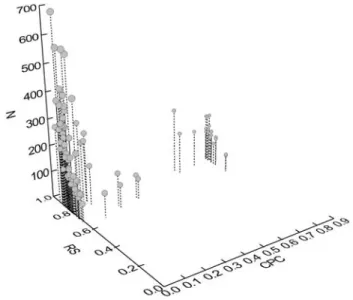
Matrix sample sizes affect the RS and the CPC meth-ods in opposite ways (Figure 2). Pairwise matrix compari-sons estimated with low sample sizes are generally less similar to one another than matrices estimated with high sample sizes using the RS method. This relationship is a re-sult of the sampling error associated with any matrix esti-mation and results in greater random error in the estimates of matrix elements in comparisons made using smaller samples. This is the same pattern was found by Steppan (1997) in his rarefaction analysis of the matrix correlation using Mantel’s test and also discussed by Cheverud (1996) in the context of matrix estimation reliability.

Conversely, for the CPC method, matrices estimated with higher sample sizes reject the null hypothesis of simi-larity more frequently than matrices with relatively lower sample sizes. Because the CPC model takes into account sample size in deriving theχ2

probabilities, the main effect of increasing sample size is to increase the power of the method to reject common structure. This is apparent in the

SaguinusxCallithrixcase analyzed in detail here. In this

case, even if the maximum likelihood matrices recon-structed under the equality and all steps below in Flury’s hi-erarchy are nearly identical to the original matrices, all three approaches for choosing an appropriate model in CPC analysis indicate that those matrices are unrelated in their structure. Conversely, the RS method indicates that covariance structure is really quite similar. With large sam-ple sizes even small differences in the variance/covariance structure of the matrices leads to statistically significant CPC tests, even when the differences are biologically triv-ial. Unlike the usual null hypothesis of no structure, CPC procedure has as its null, identical structure. The surest way to avoid obtaining significant structural diversity is to use inadequate sample sizes. With large sample sizes, it is quite possible for matrices that are indeed very similar, to be found significantly different from each other. Both meth-ods behave as expected statistically, but it is clear that a CPC result of “unrelated” matrix structures can be obtained even in situations in which the matrices are nearly identical (r > 0.9). A similar conclusion concerning CPC was reached by Houleet al.(2002) on the basis of simulation re-sults.

The above discussion suggests that future applica-tions of CPC to studies of matrix evolution face something of a dilemma. To what extent are statistically significant differences between the matrices compared biologically meaningful? For example, at first sight the comparison us-ing the CPC technique suggests that in general there is very little shared covariance structure among Neotropical pri-mate genera. This result indicates that attempts to recon-struct past evolutionary forces operating to differentiate phenotypic means of populations will be questionable given the violation of the basic assumption of constant or proportional within-group variance/covariance structures. However, while statistically significant differences among Platyrrhine covariance matrices are detected by CPC, a closer examination suggests that those differences are triv-ial or insignificant from a biological point of view as dem-onstrated by the Saguinus-Callithrix comparison. In two previous studies comparing variance/covariance and corre-lation patterns using CPC and matrix correcorre-lation this con-flict between statistical and biological significance was apparent (Steppan 1997, Ackermann and Cheverud 2000). Steppan (1997) found that while matrix correlation results indicate a high similarity among covariance structures for skull traits of several populations and species of the rodent genusPhyllotys, CPC analyses indicates that there is very little shared structure. Ackermann and Cheverud (2000) also employed matrix correlation and CPC for comparing tamarin (Saguinus) species and found discrepancies be-tween the results of both techniques.

We stress here that researchers should follow Phillips and Arnold’s (1999) suggestion to inspect closely the CPC model reconstructed matrices at each step in the hierarchy to confirm how well those matrices fit the original ones.

erwise, one could be misled into thinking that rejection of a common covariance structure among populations using CPC means that the covariance patterns are indeed unre-lated. While significantly different statistically, this differ-ence may not be biologically meaningful in the evolution-ary context. The influence of sample size and number of traits on hypothesis testing in CPC analysis should be ad-dressed by a power analysis (Patrick Phillips personal com-munication). Power is the probability of rejecting the null hypothesis when it is false and the alternative hypothesis is correct (Sokal and Rohlf 1995). However, even when power curves become available for CPC tests (Phillips 1998) the careful inspection of original and reconstructed matrices seems to be prudent in judging CPC results.

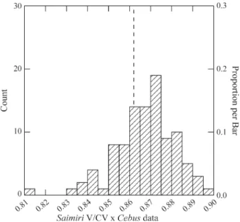
The Random Skewers method presented here could be a useful method for comparing variance/covariance ma-trices. First, the RS method, like matrix correlation, gave an easily interpretable statistic that is also continuously dis-tributed and approximately normal and reflects the overall similarity in covariance structure (Figure 3). While in the-ory the value of the vector correlation ranges from zero (orthogonality) to one (collinearity) in practice matrix ele-ments are estimated with some degree of error because they are only estimates, not population values. This limits the maximum observable correlation between estimated matri-ces. Matrix repeatability, which is the proportion of the variance in the observed elements due to variation in the true population values, can be used to set upper limits for the maximum average correlation which can be expected between estimated matrices (see Cheverud 1996). Second,

fore is particularly attractive for evaluating whether or not two variance/covariance matrices are similar enough to al-low selection gradients to be reconstructed. This is because given any fixed selection vector, if two matrices are similar, the direction of evolution specified by each matrix in re-sponse to this vector should also be similar. Third, unlike CPC, which is strongly influenced by the number of traits in the matrices, the RS method like matrix correlation is not. The only influence is that, as already noted, with more traits included the accuracy of the matrix, as an overall structure description should also increase, which is a bio-logically attractive perspective.

Finally, RS is appropriate for comparing vari-ance/covariance matrices, where matrix correlations fol-lowed by Mantel’s test is not. Although matrix correlation has been used for comparing variance/covariance matrices (Lovsfold 1986, Arnold and Phillips 1999) they are not suited for randomization tests where the matrix elements are shuffled because patterns of covariance are measured on a different scale for each row (and associated column). Usually larger traits will also present larger variances where the reverse is true for traits with smaller absolute val-ues. This scale dependency of variances and consequently the associated covariances mean that variance/covariance matrix elements are not interchangeable. While RS still has the advantage of being a distribution free method, based on extensive re-sampling, matrix elements are not exchanged. Instead, re-sampling is accomplished by applying random selection vectors upon the matrices compared and then measuring their expected evolutionary responses.

Acknowledgements

This research was supported by grants from the Con-selho Nacional de Pesquisas (CNPq), Fundação de Amparo à Pesquisas do Estado do Rio de Janeiro (FAPERJ), Fun-dação de Amparo a Pesquisa do Estado de São Paulo – Biota São Paulo (FAPESP), Fundação José Bonifácio (FUJB), Projeto de Conservação e Utilização Sustentável da Diversidade Biológica (PROBIO), an American Mu-seum of Natural History Collections Study Grant, a fellow-ship from the Conselho Nacional de Pesquisas (CNPq) and NSF grant SBR-9632163. We also thank Liam Revell for access to his programs for matrix compasrison analysis. We are grateful also for the two anonymous reviewers for their helpful comments and suggestions.

References

Ackermann RG and Cheverud JM (2000) Phenotypic covariance structure in tamarins (GenusSaguinus): A comparison of variation patterns using matrix correlation and common principal component analysis. Am J Phys Anthropol 111:489-501.

Figure 3- Example of distribution properties of the RS correlation. In this case theSaimiricovariance matrix is compared to a series of matrices gen-erated via Monte Carlo from a covariance matrix based on theCebus

Arnold SJ and Phillips PC (1999) Hierarchical comparison of ge-netic variance-covariance matrices. II. Coastal-island diver-gence in the garter snake,Thamnophis elegans. Evolution 53:1516-1527.

Begin M and Roff DA (2001) An analysis of G matrix variation in two closely related cricket species,Gryllus firmusandG. pennsylvanicus. J Evol Biol 14:1-13.

Begin M and Roff DA (2003) The constancy of the G matrix through species divergence and the effects of quantitative genetic constraints on phenotypic evolution: A case study in crickets. Evolution 57:1107-1120.

Begin M and Roff DA (2004) From micro- to macroevolution through quantitative genetic variation: Positive evidence from field crickets. Evolution 58:2287-2304.

Begin M, Roff DA and Debat V (2004) The effect of temperature and wing morphology on quantitative genetic variation in the cricket,Gryllus firmus, with an appendix examining the statistical properties of the Jackknife-MANOVA method of matrix comparison. J Evol Biol 17:1255-1267.

Cheverud JM (1984) Quantitative genetics and developmental constraints on evolution by selection. J Theor Biol 110:155-171.

Cheverud JM (1988) A comparison of genetic and phenotypic correlations. Evolution 42:958-968.

Cheverud JM (1995) Morphological integration in the saddle-back tamarin (Saguinus fuscicollis) cranium. Am Nat 145:63-89.

Cheverud JM (1996) Quantitative genetic analysis of cranial mor-phology in the cotton-top (Saguinus oedipus) and sad-dle-back (S. fuscicollis) tamarins. J Evol Biol 9:5-42. Flury B (1988) Common Principal Components and Related

Multivariate Models. Wiley, New York, 258 pp.

Houle D, Mezey J and Galpern P (2002). Interpretation of the re-sults of common principal components analyses. Evolution 56:433-440.

Lande R (1979) Quantitative genetic analysis of multivariate evo-lution, applied to brain: Body size allometry. Evolution 33:402-416.

Lande R and Arnold SJ (1983). The measurement of selection on correlated characters. Evolution 37:1210-1226.

Lovsfold D (1986) Quantitative genetics of morphological differ-entiation inPeromyscus. I. Tests of the homogeneity of

ge-netic covariance structure among species and subspecies. Evolution 40:559-573.

Manly BFJ (1991) Randomization and Monte Carlo Methods in Biology. Chapman and Hall, New York, 281 pp.

Marroig G and Cheverud JM (2001) A comparison of phenotypic variation and covariation patterns and the role of phylogeny, ecology and ontogeny during cranial evolution of New World Monkeys. Evolution 55:2576-2600.

Phillips PC (1998) CPC: Common Principal Components Analy-sis. University of Oregon, Eugene, OR. Software available at: dawrkwing.oregon.edu/~pphil/software.html.

Phillips PC and Arnold SJ (1999) Hierarchical comparison of ge-netic variance-covariance matrices. I. using the Flury hierar-chy. Evolution 53:1506-1515.

Roff DA (1995) The estimation of genetic correlations from phenotypic correlations: A test of Cheveruds conjecture. Heredity 74:481-490.

Roff DA (1996) The evolution of genetic correlations: An analy-sis of patterns. Evolution 50:1392-1403.

Roff DA (2002) Comparing G matrices: A MANOVA approach. Evolution 56:1286-1291.

Roff DA, Mousseau TA and Howard DJ (1999) Variation in ge-netic architecture of calling song among populations of

Allonemobius socius,A. fasciatus, and a hybrid population: Drift or selection? Evolution 53:216-224.

Shaw FH, Shaw RG, Wilkinson GS and Turelli M (1995) Changes in genetic variances and covariances: G whiz! Evolution 49:1260-1267.

Sokal RR and Rohlf FJ (1995). Biometry. Freeman Press, San Francisco, 850 pp.

Steppan SJ (1997) Phylogenetic analysis of phenotypic cova-riance structure. I. Contrasting results from matrix correla-tion and common principal component analyses. Evolucorrela-tion 51:571-586.

Steppan SJ, Phillips PC and Houle D (2002) Comparative quanti-tative genetics: Evolution of the G matrix. TREE 17:320-327.

Turelli M (1988) Phenotypic evolution, constant covariances and the maintenance of additive variance. Evolution 43:1342-1347.

Waitt DE and Levin DA (1998) Genetic and phenotypic correla-tions in plants: A botanical test of Cheverud’s conjecture. Heredity 80:310-319.