THE USE OF ANALYTICAL HIERARCHY PROCESS IN SPATIAL DECISION SUPPORT SYSTEM FOR LAND USE MANAGEMENT

(1)

i

THE USE OF ANALYTICAL HIERARCHY

PROCESS IN SPATIAL DECISION SUPPORT

SYSTEM FOR LAND USE MANAGEMENT

A case study of the Zambezi river valley in

Mozambique

(2)

ii

THE USE OF ANALYTICAL HIERARCHY PROCESS IN

SPATIAL DECISION SUPPORT SYSTEM FOR LAND USE

MANAGEMENT

A case study of the Zambezi river valley in Mozambique.

Miguel Antão Carrilho

mcarrilho@isegi.unl.pt

NOVA Information Management School,

Universidade Nova de Lisboa,

Lisbon, Portugal.

Supervised by

Marco Painho, PhD

Professor, NOVA Information Management School,

Lisbon, Portugal.

Co-Supervised by

Óscar Belmonte Fernández, PhD

Professor, Universitat Jaume I

Castellon, Spain.

Joel Dinis Silva, MSc

NOVA Information Management School,

Lisbon, Portugal.

(3)

iii

ACKOWLEDGEMENTS

I would like to acknowledge that, Joel Dinis my co-supervisor, was a restless support

on the development of this thesis. Joel Dinis is one of the brightest minds I had the

joy of meeting, and with his guidance and shared knowledge I was able to finish the

work here presented.

I must also recognize the constant supervising, and motivational spirit of Professor

Marco Painho, contributing to a constant improvement of the work presented. This

work had also the tremendous support of my friends and colleges Tiago Oliveira,

Alexandre Baptista, Luis Almeida, Otávio Sian, Hugo Martins and Bezaye Tesfaye.

I would also like to acknowledge that, without my family, my mother Manuela

Antão, brother, Pedro Carrilho and father Orlando Carrilho I would not have a

motivation to fulfill this work. I would also like to recognize the great support and

dedication of Vanessa Ligeiro, as my companion and best friend. I would like to

thank also my friends and colleges of this master, for the support during this year and

half of hard work. I would like to dedicate this work to my friend Gonçalo Amor,

thus he remembers everyday what he fights for.

“I believe that the very purpose of our life is to seek happiness.” – Tenzin Gyatso

(4)

iv

THE USE OF ANALYTICAL HIERARCHY PROCESS IN

SPATIAL DECISION SUPPORT SYSTEM FOR LAND USE

MANAGEMENT

A case study of the Zambezi river valley in Mozambique.

ABSTRACT

Geographic information systems give us the possibility to analyze, produce, and edit

geographic information. Furthermore, these systems fall short on the analysis and

support of complex spatial problems. Therefore, when a spatial problem, like land

use management, requires a multi-criteria perspective, multi-criteria decision

analysis is placed into spatial decision support systems. The analytic hierarchy

process is one of many multi-criteria decision analysis methods that can be used to

support these complex problems. Using its capabilities we try to develop a spatial

decision support system, to help land use management. Land use management can

undertake a broad spectrum of spatial decision problems. The developed decision

support system had to accept as input, various formats and types of data, raster or

vector format, and the vector could be polygon line or point type. The support system

was designed to perform its analysis for the Zambezi river Valley in Mozambique,

the study area. The possible solutions for the emerging problems had to cover the

entire region. This required the system to process large sets of data, and constantly

adjust to new problems’ needs. The developed decision support system, is able to

process thousands of alternatives using the analytical hierarchy process, and produce

(5)

v

KEY WORDS

Analytical Hierarchy Process

Geographic information systems

Spatial Decision Support Systems

(6)

vi

ACRONYMS

AHP - Analytic Hierarchy Process

CR - Consistency Ratio

CI - Consistency Index

IR - Index of Randomness

GDAL - Geospatial Data Abstraction Library

GI - Geographic Information

GIS - Geographic Information System

LLSM - Logarithmic Least Squares Method

MCDA - Multi-criteria Decision Analysis

PBO - Purpose-built offices

PROMETHEE- Preference Ranking Organization Method for Enrichment

Evaluations

SDSS - Spatial Decision Support System

(7)

vii

INDEX OF TABLES

Table 1 Saaty (1987) pairwise comparison of the criteria college example ... 9

Table 2 Saaty (1987) alternatives pairwise comparison matrix college example. ... 10

Table 3 Beigbabayi et al. (2012) alternatives table for humidity sub-criteria. ... 12

Table 4 Grading Scale explanation ... 20

Table 5 Grading table example. ... 20

Table 6 Grading table example. ... 21

Table 7 Soil type grading table. ... 28

Table 8 Population density grading table. ... 28

Table 9 Slope grading table. ... 28

Table 10 Overall grading table of the alternatives. ... 29

Table 11 User's input description... 47

Table 12 Grading tables used in the example, reallocation of Tete city. ... 51

Table 13 Grading tables used in the example, reallocation of Tete city. ... 51

Table 14 Example matrix with priority vector and row. ... 53

Table 15 Saaty's (1990) fundamental scale of comparison... Annex, 59

(9)

ix

INDEX OF FIGURES

Figure 1 Hierarchy for choosing college example (Saaty, 1987). ... 8

Figure 2 Overview flowchart of the system design. ... 18

Figure 3 Flowchart of the geographic process ... 19

Figure 4 Flowchart of the AHP computation ... 25

Figure 5 Detailed flowchart of the AHP system design. ... 26

Figure 6 Example alternatives. ... 27

Figure 7 Folder structure of the application software. ... 38

Figure 8 User interface of the application software, in development. ... 39

Figure 9 Context image of the study area. ... 41

Figure 10 Administrative divisions of the study area. ... 42

Figure 11 Land cover map of the study area. ... 43

Figure 12 Rivers, reservoir and slope of the study area. ... 44

Figure 13 Hierarchic structure of the problem. ... 49

Figure 14 Alpha file used in the example, reallocation of Tete city. ... 49

Figure 15 Geo file used in the example, reallocation of Tete city. ... 50

Figure 16 Raster overlay illustration. ... 52

(10)

1

1. INTRODUCTION

Geographic Information Systems (GIS) are used to manipulate, summarize, query,

edit and visualize geographic information (Goodchild, 1992). Geographic

information science was established because geographic information has unique

properties and problems (Goodchild, 1992). Some individuals such as Ratti (2005)

tend to see geographic information science as a modern approach to Geography.

Longley et al (2010) argue that geographic information science was born in

London, due to a cholera outbreak studied by John Snow in 1854. John Snow

related the location of water wells to cholera outbreaks. The geographic

perspective of problems is sometimes the key to the solution, like the cholera

outbreak of 1854 in London.

GIS started to be used in the 1960’s (Goodchild, 1993). The first GIS was

developed in Canada for land inventory (Tomlinson, 1962), due to the vast

measurements needed for the project. The only cost-efficient alternative was a

computer based system (Goodchild, 1993). The role of GIS in many facilities’

management systems provide a different perspective to data (Goodchild, 1992).

Accessing different data types at the same time is another problem that stands for

the use of GIS (Goodchild, 1993). The GIS are used for various purposes, such as

land use management (Malczewski, 2006).

When it comes to land use planning, projects like the location of a future power

plant or the reallocation of a city are a reality. These decisions call for several

perspectives, because they affect third-party interests. This type of problems tend

to involve several organizations, governmental, environmental and private

corporations to make the final decision on the location. These decisions are made

to achieve medium or long-term goals and need to be based on concrete evidence.

Thus lots of spatial data is needed. For example, hydrology data, soil type data,

soil price data, connections to industry supply chains like ports, main power lines,

etc. Hence these type of decisions depend on a large number of criteria. For these

reasons, land use management is a very complex task, justifying the need for the

integration of a Multi-criteria Decision Analysis (MCDA) as a component of a

SDSS (Marinoni, 2004). The use of MCDA in GIS has been widely studied (Lin

(11)

2

2013; Sugumaran & DeGroote, 2011). Decisions are the result of comparing

alternatives over one or more criteria, that are relevant for the problem (Marinoni,

2004). They are results of an instinctive weighting process. Therefore the MCDA

used, had to be intuitive in the decision thinking, requiring weight assigning, and

an intuitive structure of the decision. The MCDA method found to cover these

points was the Analytic Hierarchy Process (AHP) (Saaty, 1990).

The application software was developed to be part of the environmental strategic

evaluation of the multi-sectorial plan for land use management of the Zambezi

river Valley. This project has the final goal of helping land use planners make

better evidence based decisions. This goal is assisted by a web-based GIS of the

study area, part of the Zambezi river basin in Mozambique. To complement the

decision making process the web-based GIS needed to be assisted by a decision

support system. Since decisions are primarily spatial, a Spatial Decision Support

System (SDSS) is the most suitable tool for these decision makers (Malczewski,

2006). Since the web-based GIS was planned to support all types of data, from

vector type to raster type, and from all possible topics, from geology maps to

population density maps, the SDSS had to support a broad spatial analysis

processes.

The project was designed to manage land use in any area of the globe and was

tested for the study area. Hence the resulting output of the GIS-MCDA had to

consider, impartially, alternatives over an entire study region. The solution was to

overlay a small enough grid on the area of study. With a grid format, the

alternatives number can be very high, which in AHP MCDA like methods is not

applicable (Malczewski, 2006). The idea is to develop a GIS-MCDA that is data

flexible, taking in raster or vector-format data, and produce a suitability map of

any study region, in a grid like format.

The research questions are:

1. Can the AHP be used in a SDSS, to support the diverse land use decisions

?

2. Is it possible to use open source technology to build a SDSS based on

AHP?

(12)

3

The objectives of the thesis are to:

 Test the possibility to integrate AHP in a SDSS to better support land use

related decisions.

 Test the possibility of open source technology to develop a SDSS using

AHP.

 Test the possibility of using the AHP with a large number of alternatives.

The thesis is organized in the following way: the literature review will be

presented in section 2, where an introduction to the MCDA methods in GIS will

be given and a deeper investigation of the used algorithm used will follow. The

use of the AHP in GIS will be reviewed also. In section 3 the study area and the

data available for the project will be described. Section 4 describes the

methodology used in the development of the software application. This chapter

will be divided into the requirements, the system design, the implementation and

the verification. Section 5 will describe the results and discussion of the testing

example. To finalize Section 6 will present the conclusions and possible future

(13)

4

2. LITERATURE REVIEW

This chapter will describe and characterize previous work, on the topic discussed

in this thesis. It will also describe the analytic hierarchy process which is the

MCDA used in the implementation.

2.1. Multi-criteria decision analysis in GIS

A Multi-criteria Decision Analysis (MCDA), is a decision making analysis that

will bring into the decision multiple criteria affecting it. These methods began to

emerge during the early 1970s, when researchers from the economical and

decision making fields identified weaknesses in the neoclassical view of decision

making and site location (Carver, 1991). MCDA are used in computer-based

systems called Decision Support Systems. There are many MCDA algorithms, but

they can be divided into Multi-attribute (MADA) or Multi-objective (MODA)

decision analysis (Malczewski, 1999). The MODA techniques are characterized

by a Multi-Objective problem decision. These methods are continuous, because

the best solution may be found anywhere in a feasible region. The MADA

techniques are characterized by Multi-Attribute decision problems, and are

assumed to have a predetermined number of alternatives. The AHP is classified as

a MADA technique (Malczewski, 2006).

When the decision being made has a spatial character it is called upon a Spatial

Decision Support Systems (SDSS). The efforts to integrate GIS with MCDA have

been contributory for developing the prototype of spatial decision support systems

(Goodchild, 1993). These systems integrate the GIS with DSS to solve problems

with a spatial dimension (Silva, Alçada-almeida, & Dias, 2014). The use of

Multi-Criteria Decision Analysis in Geographic information Science has been widely

applied and used since 1986 (Sugumaran & DeGroote, 2011). Carver (1991) is

one of the most cited and one of the first researchers to apply the MCDA methods

to GIS (Malczewski, 2006). The blooming of this combination came around the

year 2000 with the broader use of technology, the recognition of the decision

analysis and support systems by the GI Science community, and also resultant of

the lower costs and user-friendly MCDA software (Malczewski, 2006). MCDA

(14)

5

Marinoni, 2004; Massei, Rocchi, & Paolotti, 2013; Sugumaran & DeGroote,

2011). Some of those researches are:

 A decision support system for optimizing dynamic courier routing (Lin et

al., 2014).

 Development of a web-based multi-criteria spatial decision support system

for the assessment of environmental sustainability of dairy farms (Silva et

al., 2014).

 An exploratory approach to spatial decision support (Jankowski, Fraley, &

Pebesma, 2014).

In the first mentioned research, developed by Lin et al (2014), the topic of the research is to create a decision support system (DSS), that optimizes dynamic

courier routing operations. This work is attached to a spatial component, because

routing problems are always have a spatial relation. Therefore, even if the

research does not mention it, it has an intrinsic spatial component. The word

dynamic means that, while the courier is executing the planned route, the DSS can

exclude costumers that canceled the courier service or add new ones.

The proposed methodology to optimize the dynamic courier routing, is to

integrate a hybrid neighborhood search algorithm with a DSS. After reviewing the

literature on the scope of the research, the researchers conclude that there is

potential for developing a DSS integrating a dynamic vehicle routing model. The

proposed hybrid neighborhood search algorithm is composed of a heuristic

method called IMPACT, a Variable Neighborhood Search (VNS), and a removal

insertion heuristic. The IMPACT heuristic measures the three criteria for

measuring the impacts that a costumer has on the routing of the courier. The own

impact, the closeness between the time of starting the courier service and the

earliest service time. The external impact, the affected difference of time window

of un-routed costumer j if costumer c right before or after j. And the internal

impact, defined by the distance increase, time delay and time gap, if consumer c is

inserted between i and j. The VNS is used to improve the initial solution, obtained

with IMPACT. This algorithm intends to optimize the number of couriers by

using intra-route and inter-route searching processes. The final heuristic is used to

(15)

6

costumers that have been inserted in the routing plan, and reinserting these with

the new costumers excluding the canceled ones, this heuristic is able to redo the

routing plan dynamically while the courier is executing his route. The research

concludes that the hybrid neighborhood search approach is able to minimize

traveling distance with fewer vehicles. It also concludes that for real-time

environment it is an appropriate algorithm for decision making.

Another research reviewed tries to assess the environmental sustainability of dairy

farms in a Portuguese region using a Web-based MCDA method in ArcGIS

software. It proposes the use of a specific MCDA method, ELECTRE TRI. The

research focuses on the main Portuguese milk production area,

Entre-Douro-e-Minho.

The methodology proposed is the use of a Web MC-SDSS as a fully dynamic

GIS-MCDA integration. This means the interface is completely integrated in a

single system. The GIS platform used is the GIS proprietary software ArcGIS 9.3.

The ELECTRE TRI method is an outranking MCDA approach. It is based on the

pairwise comparisons between potential alternatives. The comparisons use an

outranking relation, where one alternative outranks another if the former is

considered, “not worse than” the latter. ArcGIS provides a macro development

environment using Visual Basic for Applications (VBA) programming language

allowing to extend its functionalities. The researchers conclude that the

user-interface for configuration, prediction, visualization, and analysis of the model is

user-friendly. The interface is the same for all procedures allowing a uniform,

transparent and less technical effort demanding process from decision makers.

To finalize the review on diverse MCDA methods used in GIS a more complex,

yet simplistic approach will be reviewed. The research by Jankowski et al (2014),

attempts to solve problems with spatially-explicit decision variables, multiple

objectives, and auxiliary criteria preferences. This research proposes the

combination of two MCDA, a fuzzy logic system and a spatially adaptive genetic

algorithm. The Fuzzy logic system, is based on a Multi-objective algorithm

MOGA, a Multi-objective Genetic Algorithm. Firstly MOGA solves a

mathematical optimization model achieving a Pareto non-denominated solution

(16)

7

trade-offs between the selected Pareto-optimal solutions. Once the decision maker

selects candidate solutions, these are evaluated as a multi-criteria decision

problem. The research does not suggest a specific MCDA algorithm, instead it

states that for each purpose the pros and cons of the algorithms should be

evaluated. And adds the fact that spatial explicit criteria should be used in this

final step of the decision. The researchers conclude that this approach can be

applicable to a broader variety of problems.

2.2. Analytic hierarchy process

The MCDA approach used in this thesis is the Analytical Hierarchy Process

(AHP). The AHP was developed by Tomas L. Saaty in 1980, and as a

multi-criteria decision making analysis arranges the factors in a hierarchic structure. The

structure is composed of an overall goal to criteria, sub-criteria, and alternatives.

This hierarchic arrangement serves two purposes: first, it provides an overall view

of the problems complexity; and secondly it helps decision makers assess whether

the issues in each level of the hierarchic structure are in the same order of

magnitude, so that decision maker can compare these elements accurately (Saaty,

1990). The advantage of the AHP over other multi-criteria decision support

methods is that it takes into account the decision maker’s intuitive knowledge into

the analytical decision (Saaty, 2000). The idea behind the AHP is to clearly define

the decision being made and the criteria that affect it. To use the AHP, one should be familiar with the decision’s subject (Saaty, 1990). The decision affecting criteria should be defined by experts on the problem’s subject.

The AHP is arranged into two parts, the structure of the problem, and the

weighting of the various parts of the problem’s structure. Firstly the decision

maker must decompose the decision in hierarchical sub-problems easier to

understandable (Saaty, 1987). The hierarchy elements can be related with any aspect of the decision’s subject, tangible or not, precisely measured or not; in other words, anything associated to the decision. The criteria should be chosen by

an expert on the subject, representing reliably the real affecting factors of the

decision. When the problem is, what stock to buy, one can ask a student of

economics, what is his opinion on the factors affecting the problem. On the other

(17)

8

the decision maker has to define what is the focus of the decision, the criteria, and

if needed, sub-criteria that affect the decision. Finally the possible alternatives for

the decision.

Secondly the decision makers must evaluate the various elements systematically, comparing them to one another, in pairs. This comparison is done using Saaty’s fundamental scale of comparison ranging from 1 to 9, see table 1 in annex (Saaty,

1987). This scale of importance defines the value 1 as factors having “equal

importance”, and 9 defines “extreme importance” of a factor over another factor. The decision maker will have to pairwise compare the criteria and sub-criteria

defined. And also the alternatives according to each of the criteria defined. Saaty

(1987) gave an easily understandable example and illustration of this process. His

example expresses the decision of a high school student wanting to go to college,

and does not know what college to choose. So the structure of this decision is

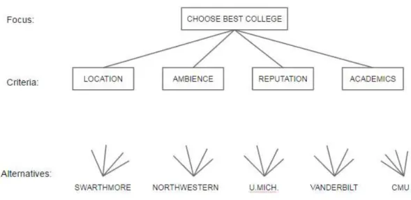
illustrated in figure1:

Figure 1 Hierarchy for choosing college example (Saaty, 1987).

As you can see the main goal of the decision is to choose the best college. The

criteria that affect this decision are: Location, Ambience, Reputation and Academics. Where Location, is perceived as the farther away from the student’s home the better. Ambience, expresses how happy the student felt at the university.

Reputation, represents how the university is rated. And Academics representing

(18)

9

this case is the decision maker, also defined the possible alternatives to the final

decision: Swarthmore College, Northwestern University, the University of

Michigan, Vanderbilt University and Carnegie-Mellon University. After

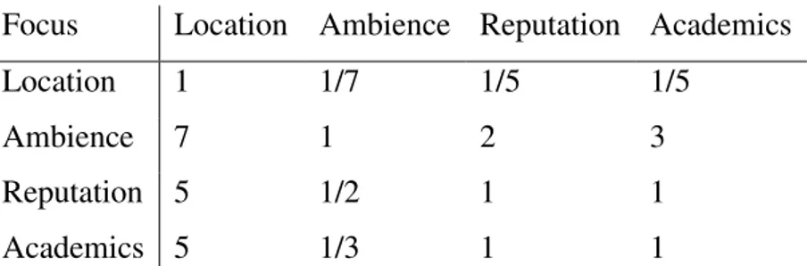
structuring the decision into a hierarchy, the next step is to execute the pairwise comparison of the criteria using Saaty’s fundamental scale, resulting into a pairwise comparison matrix, in table 1.

Focus Location Ambience Reputation Academics

Location 1 1/7 1/5 1/5

Ambience 7 1 2 3

Reputation 5 1/2 1 1

Academics 5 1/3 1 1

Table 1 Saaty (1987) pairwise comparison of the criteria college example

When the comparison of all criteria with all criteria is done, the result is a

pairwise comparison matrix. This matrix is called reciprocal matrix. This is due to

the procedure used to compare the factors, in this case the criteria. The decision maker will compare Ambiance against Location, and it’s intuitive, or subjective,

judgment is translated into a value of Saaty’s fundamental scale of comparison.

The value the student decided to input was 7. This means that, the Ambience of a

university is strongly favored and its dominance over the Location criterion is

demonstrated in practice, see table 1 in annex. In the opposite comparison the

reciprocal value is entered. To verify that the values are not entered randomly, a

matrix has to respect the consistency condition, . Although the matrix

above does not respect this principle its inconsistency can still be acceptable. This

is verified with the consistency ratio. The consistency ratio is based on the

permissive that although, , this difference is compensated by other

differences. Some differences are above the expected value and some are below

the expected value. If they mitigate each other up to a certain point 0.9 then the

matrix can be accepted as input (Malczewski, 1999). This ratio can be calculated,

(19)

10

Ratio (CR) is less than 0.10 the ratio indicates a reasonable level of consistency in

the pairwise comparisons, meaning the matrices are acceptable. With a reasonably

consistent comparison matrix the next step is to calculate the eigenvectors of the

matrix. The Eigenvectors give the decision maker an overview of his pairwise

comparisons in the form of priorities (Saaty, 2000). This priorities of the criteria

establish an order of importance magnitude for the decision. The following step

for the decision maker is to build the pairwise comparison matrices of the

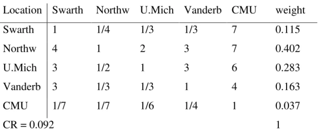
alternatives according to a specific criterion. Following the example, exposed by

Saaty (1987), an example of the pairwise comparison matrix of the schools

according to locations, in table 2.

Location Swarth Northw U.Mich Vanderb CMU weight

Swarth 1 1/4 1/3 1/3 7 0.115

Northw 4 1 2 3 7 0.402

U.Mich 3 1/2 1 3 6 0.283

Vanderb 3 1/3 1/3 1 4 0.163

CMU 1/7 1/7 1/6 1/4 1 0.037

CR = 0.092 1

Table 2 Saaty (1987) alternatives pairwise comparison matrix college example.

In this example we can see that the alternatives are being compared against each

other but according to one of the criteria defined, Location. For example,

Northwestern University, according to Location, is 4 times more desirable than

Swarthmore College. And reciprocally Swarthmore College has ¼ of the desirable

Location than Northwestern University. The consistency ratio and the

eigenvectors are calculated for the alternative’s matrix, as they were for the

criteria matrix. This process is done for all criteria, meaning there will be as much alternative’s pairwise comparison matrices as the number of criteria, because for all criteria the alternatives are pairwise compared. This will give the student, the decision maker, an overview of the alternatives’ priorities. Obtaining the priorities of the criteria and the priorities of the alternatives considering each criteria, the

(20)

11

notice that, the eigenvectors’ values are the priorities. This multiplication results into a ranking of the alternatives or the global priority vector for the alternatives

(Saaty, 1990), see equation 1.

(1)

With a better understanding of the MCDA used in this research its uses in GIS

could give a better insight and understanding of the advantages of this

combination this will be discussed in the following section.

2.3. Analytic hierarchy process in GIS

The study of the integration of the MCDA, Analytical Hierarchy Process in GIS

has been broadly researched (Malczewski, 2006). The topics being reviewed here

are, agriculture (Beigbabayi, Mobaraki, Branch, & Branch, 2012), environmental

(Ying et al., 2007) and locational evaluation (Safian & Nawawi, 2012). The last

research reviewed will be the implementation of a AHP tool within GIS

environment (Marinoni, 2004).

The first research focuses on the agriculture topic, scopes the evaluation of site

suitability for Autumn Canola cultivation in the Ardabil province in Iran

(Beigbabayi et al., 2012). To assess site suitability, the spatial modeling is one of

the strategies that allow its scientific evaluation (Beigbabayi et al., 2012). The

researchers state that different factors must be taken into account when evaluating

site suitability, requiring for a MCDA. The MCDA chosen was the AHP because

of its accuracy. The researchers defined a series of criteria that influence the

cultivation of Autumn Canola. From these criteria a series of sub-criteria were

defined. For example, for the climate criterion, the frost, precipitation and

humidity were defined as some of the sub-criteria. The alternatives were pairwise

compared according to each of the sub-criteria. It is of important notice, that the

(21)

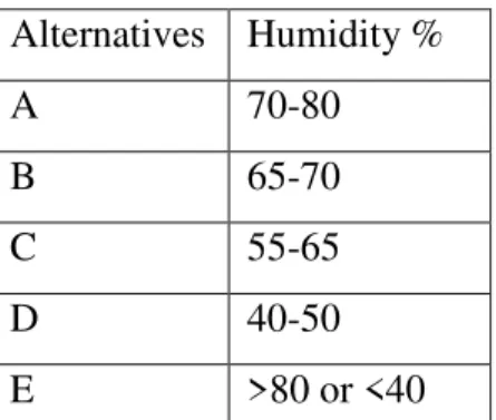
12

intervals of the sub-criteria defined. Taking the sub-criterion humidity, the

alternatives were defined as follows:

Alternatives Humidity %

A 70-80

B 65-70

C 55-65

D 40-50

E >80 or <40

Table 3 Beigbabayi et al. (2012) alternatives table for humidity sub-criteria.

This way of structuring the alternatives is very intersting because it is independent

from the alternative’s area, or number. The comparisons of the alternatives were

based on the best known conditions for the cultivation of Autumn Canola. The

comparison matrices of the criteria, sub-criteria, and alternatives were tested for

their consistency, and the eigenvectors were calculated. The priorities were

obtained for all criteria, sub-criteria and alternatives. After the priorities were

defined, these were matched with the corresponding geographic data of the

Ardabil province. The province’s suitability for the cultivation of the Autumn

Canola was devided into five categories. These categories liked to the

corresponding geographic data provided the researchers the overview of site

suitability for Autumn Canola cultivation. The GIs software used was ArcGIS 9.3.

The next research reviewed mentions the benefits of using AHP in GIS to

evaluate the eco-environment quality in the Hunan province of China (Ying et al.,

2007). In this research the criteria has four hierarchical levels, where sub-criteria

from one level relate to criteria of the level directly above. The main goal is to

evaluate the Eco-environmental quality of the 88 counties that make up the Hunan

province, this makes it the first level of the hierarchy. The second level is divided

in 4 aspects of the environmental quality assessment. The third level is divided

into 15 levels that relate to the ones above. The fourth level is dived into 28

sub-sub-criteria that are also directly related to the sub-sub-criteria above. The comparison

(22)

13

Experts’ advice was taken to correctly compare the criteria. The alternatives in this research, contrary to the previous, are the 88 counties that make the Hunan

province of China. The alternatives’ eco-environmental quality was assessed by

using a synthetic index and sub-index. The synthetic evaluation of each county

was the sum of the corresponding weight values of all related factors.

It is mentioned in the research that the combination of AHP with GIS is useful for

this study, because the AHP has the advantage in multi-indexes evaluation and the

GIS is good at spatial analysis.

For this research as for the previous a consistency ratio was calculated to measure

the consistency of the pairwise comparison matrices, reassuring the

non-randomness. Once again the use of the proprietary software ArcGIS is mentioned.

The next research reviewed uses AHP and GIS on the evaluation of locational

characteristics quality for purpose-built offices in Malaysia (Safian & Nawawi,

2012). The term Purpose-Built Office (PBO), meaning an office designed and

constructed to serve a particular purpose. The evaluation focused on 5 PBOs

within the Kuala-Lumpur Golden triangle. The combination of a GIS with AHP

provides an effective evaluation on PBOs and can be profiting.

To overcome the problem of the locational analysis covering spatial and

non-spatial data it was proposed the technique of combining AHP with GIS. The

research involved two phases of analysis, the AHP and the GIS. The AHP was the

first phase. It was used to identify the quality level of locational characteristics on

PBOs. The researchers required the help from respondents to assess this

characteristics. Five characteristics were determined by presenting a questionnaire

form to PBO’s tenants. These represent the criteria, they were location of

commercial features, availability of transport options, transportation and parking

places, vehicle flow and efficiency of property market. The tenants of each PBO,

were then asked to weight the importance of the locational characteristics, using Saaty’s fundamental scale.

The second phase used a GIS with a network analysis method. A locational

quality index was used in order to evaluate the distances, based on the network

(23)

14

technique was applied. A locational quality index is used to assess the evaluation

on locational characteristics of the PBOs.

The final research being reviewed focuses on the implementation of the AHP in

ArcGIS software as an extension of the tools provided (Marinoni, 2004). The

AHP was implemented using a visual basic programing language in ArcObject.

ArcObject is an ESRI software to develop Macros using visual basic programing

language for applications. The Macro developed is to be used in ArcGIS

environment. The decision to use VBA (visual basic for applications) macros was

based on integration capabilities with ArcGIS. Some of them are the use of

ArcGIS functionality to its full extent, VBA macros can take advantage of global

variables, and the creating, testing and debugging similarity of ArcGIS VB editor

to other VB development environments.

The Macro developed accepts all criteria considered relevant as long as it is

regionalized and in raster format data set. The user also has to do the necessary

transformations to have all raster data sets in the same scale. Each criterion has to

be represented with a raster image map. The raster images values need to be in the

same scale. Although a standardized scale is not provided the researcher suggests

the definition of intervals within the raster values. The values the decision maker

considers bad should have the value 0, while better values should be classified

with higher values.

The macro developed also helps the decision maker by filling in the reciprocal

values in the pairwise comparison matrix of the criteria. The eigenvectors are

calculated using an eigenvector calculation routine. Finalizing the process, all

classified raster images are multiplied with their corresponding weight and

summed up. Each raster cell is calculated according to the classifications done

previously. The resulting raster is added to the ArcGIS environment, representing

the suitability zones, with respect to the specific land use.

The macro also uses a spatial analyst functionality of ArcGIS. If requested the

macro will perform the conversion of the raster image into a polygon vector

format. The macro assumes the raster images have the same resolution and extent,

meaning the perfect overlap of the criteria raster and the resulting raster. The

(24)

15

facilitate land use assessment. The presented VBA macro fills the gap since a

commonly used GIS, ArcGIS, does not provide this functionality. The macro is

intended to provide a template for users who are working in the field of land use

assessment, and other geosciences where regionalized criteria play a role in the

(25)

16

3. METHODOLOGY

3.1. Requirements

The guidelines to the development of software were defined as follows: (i)

execution in useful time, (ii) process big data sets of alternatives and (iii) a user

friendly way of thinking. These arose some constraints that will also be discussed

in this section.

Since the application software had a possibility of being implemented on the web

later on, the process had to be done in feasible time. The processing was broken

into two parts, initially, the processing of the geographic information was done

with a GIS, ArcGIS 10.2. This process could take from three to almost eight hours

depending on the number of alternatives and criteria that were defined as affecting

the problem. And the second part, the AHP, could take almost three more hours to

conclude. This were not acceptable for a web based application. This processes

needed to be optimized. The geographic processing of the data needed to be

automated also due to the time consuming restriction.

Another requirement is the processing of big datasets, or big sets of alternatives.

Because the alternatives for the problem had to cover the entire study area, this

meant that the number of alternatives could be very large. For example, the study

area where the AHP-SDSS was applied is approximately 149 900 km2, in the case

the user wanted a resolution of 2 by 2 km on the output map, the application

software needed to process this area divided into 4 km2 parcels. This resulted into

approximately 37 475 parcels, these being the total number of alternatives.

Additionally, with the AHP one needs to compare the alternatives in pairs,

building the pairwise comparison matrix. This process is done for all criteria.

Each comparison matrix would have about 1 404 375 625 elements times the

number of criteria. This would be a dreadful task for the decision maker. The time

spent comparing alternatives according the criteria would be immense. The

application software could not let the user do the pairwise comparisons by hand.

Therefore an automatic way of comparing the alternatives had to be implemented.

The last constraint is related to the output of the application software, this required

(26)

17

process. As the alternatives had to cover the entire area, and the suitability values

were to be presented as a percentage, the most adequate data format would be a

raster image map, where the cell values are the suitability value of that cell.

The application software as being part of the environmental strategic evaluation of

the multi-sectorial plan for land use management of the Zambezi River Valley

project had to be able to take as input all the available data layers in the

web-based GIS developed.

This guidelines and restrictions affected the application software’s development, requiring it to consider the most alternatives possible as input. Requiring

furthermore, a flexibility in the input data. Resulting into a more error-proof

(27)

18

3.2.System design

The system was designed to have 2 parts, the first organizes the input of the user,

and the second processes it into a suitability map. The first part, due to the input

flexibility need, was designed to standardize geographic data, formatting all input

data into raster format with the same resolution, reference system and extensions.

The second part processes the resulting data outputting a suitability raster format

map.

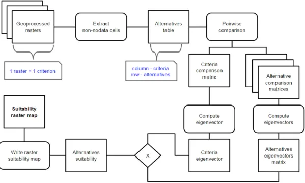
The process starts with the user input, followed by a geographic processing of

data, which goes through the AHP, resulting into an output raster, in figure 2. This

process will be detailed along this chapter.

Figure 2 Overview flowchart of the system design.

3.2.1. Geographic processing

The geographic processing of data will from now on be called geoprocess for

simplification. This process only produces standardized geographic information

for the computation of the AHP. The geoprocess depends strongly on the

Geospatial Data Abstraction Library (GDAL, 2015).

The GDAL library is used to read and write geospatial data formats, and is

released under the X/MIT style Open Source license. This library comes with a

variety of command line utilities for data processing and translation. These are the

GDAL functionalities used in the geoprocess: the vector utility program ogr2ogr

and the raster utility programs gdalwarp, gdal_rasterize and gdal_proximity.py. These programs will be discussed later in this chapter.

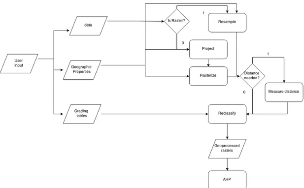
The geoprocess is illustrated in the flowchart in figure 3. This flowchart illustrates

the user input being separated into 3 parts, the data, the geographic properties and the grading tables. The data, it’s the GI layers available in the web-based GIS, either in raster or in vector format. Each layer is assumed to be a criteria of the

AHP. For example, a shapefile of the population density by districts, or a raster

(28)

19

Figure 3 Flowchart of the geographic process

The geographic properties are information needed for the GDAL programs. Like

the georeferenced extent and resolution of the output raster file, and the desired

spatial reference.

The user will need to define intervals for the geographic data values, and give

importance to these intervals, requiring therefore grading tables. Translating the

real value of data into a standard scale, where all types of data can be compared.

This grading process is used to simplify the problem of pairwise comparison,

mentioned before. The grading tables will be the translation between the

geographic data values and the grading given by the user to this values. The

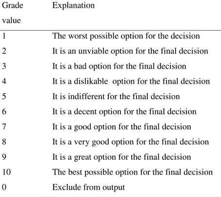
grading scale will vary only from 1 to 10 in integer numbers (see table 4), where 1

(29)

20

Grade

value

Explanation

1 The worst possible option for the decision

2 It is an unviable option for the final decision

3 It is a bad option for the final decision

4 It is a dislikable option for the final decision

5 It is indifferent for the final decision

6 It is a decent option for the final decision

7 It is a good option for the final decision

8 It is a very good option for the final decision

9 It is a great option for the final decision

10 The best possible option for the final decision

0 Exclude from output

Table 4 Grading Scale explanation

For example, using slope data, the decision maker might say, for a specific

problem, the slope values from 0% to 3% could be the best possible, and give it

the value 10 in the grading scale. From 3% to 5%, the slope would still be very

good for his final decision and give it a value of 8. On the other hand, if the slope

is higher than 5%, it would be the worst possible for his final decision giving it a

value of 1 (table 5).

Slope value (%) Grade (1 - 10)

0% - 3% 10

3% - 5% 8

>5% 1

(30)

21

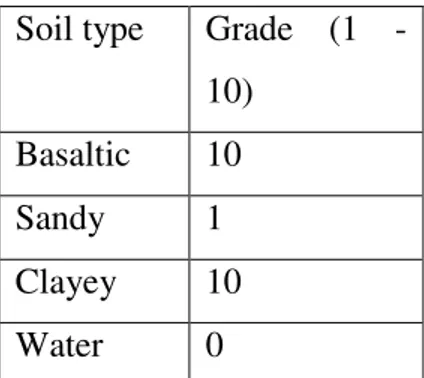
A fact about this scale is that, the user can choose 2 intervals or categories, to be

perfect for the final decision, Giving both the same value in the grading scale. For

example, if one of the criterion that affects the decision is soil type, the user can

make the following grading table (table 6).

Soil type Grade (1 -

10)

Basaltic 10

Sandy 1

Clayey 10

Water 0

Table 6 Grading table example.

Table 6 expresses that, a basaltic soil or a clayey soil, would either be the best

possible options for the final decision; and sandy soil type would be the worst

option for the final decision. One should notice the exclusion of water soil type

from the decision. This exclusion should be used carefully, regarding this soil type

will be excluded from the output. When applied, the user should have an idea of

what he is excluding from the output, because with this the user might be

excluding 50 to 90% of the study area. To exclude 50% of the study region even

before the computation of the AHP, might lead to a biased set of alternatives.

Another fact about the grading scale, is that the user doesn’t need to use the entire

scale, for each grading table, the user might use only 3 intervals as showed in

table 5. It is advised that the user still uses the entire range of values or categories

of the geographic data, because in case a certain value or category is omitted the

AHP process will assume it as excluded from the output.

After the data, the geographic properties and the grading tables are defined the

application software is ready to run. The first step is to verify which data are in

raster format and which are in vector format. If data is in raster format a resample

of the raster image will be performed by using the gdalwarp program from the GDAL. On the other hand, if data is in vector format, the application software will

(31)

22

projection is done, it will rasterize the projected vector data using gdal_rasterize

from the GDAL.

Having all data in raster format, with the same extents and resolution, the

application software will verify if it needs to perform a measurement of distances.

This is due to the possible need of specifying as a criterion, distances to, or from a

certain geographic feature. The distance intervals are graded in the grading tables

just as any other criterion. The user must specify if there is a need for the

computation of distances. If the distances are required, the application software

will resort to the gdal_proximity.py program of the GDAL library.

If there is no need for the calculation of distances, or when the distances have

been calculated, the application software will perform the reclassification. This is,

from the grading tables, for each cell in the raster images, the application software

will translate its value into the grade provided by the user. One needs to remember

that at these stage all data is in raster format, in the same coordinate system, with

the same resolution and extent, implying that the cells of all rasters overlap

perfectly. The reclassification method will use the grading tables as a translation reference. The application software will read each cell’s value and compare it with the respective grading table. For example, in the soil type example

mentioned before, at this point, we have a raster map of, let’s say, 2 by 2 km cells,

where in each cell its soil type value is defined. And according to table 7, all cells

that have the basaltic and clayey value will now have the value 10, the cells with

the value sandy will now have the value 1 and the cells with the value water will

now have the value 0. And this process is done to every cell of every raster map,

each of which represents a criterion.

The gdalwarp program is an image reprojection and warping utility. This program is used as a command line program and has 41 possible arguments to be used. The

ones being used by the application software developed are 7, them being the source file’s name and location, the target file’s name and location, the target spatial reference set, the target extent of the image, the destination nodata value,

the target resolution of the image and the quiet mode.

The source and target file’s name are written as the path in computer’s file

(32)

23

geographic data, used to make a geographic transformation or projection if

needed. This should be specified as EPSG: followed by the coordinate reference

system code of the region in study. The target image extent argument, takes in the

x axis minimum, followed by the y axis minimum, followed by the x axis

maximum, followed by the y axis maximum, extents of the raster image. This

must be expressed in the coordinate reference system units of the target raster

image. The nodata value can be -9999, since this value is not common in data.

The target raster’s resolution is the raster cells’ size. The size of the cell defines,

the resolution of the raster. This argument should be represented in the unit of

measurement of the target coordinate reference system and as x axis first and y

axis second. The quiet mode, states that while running, unless there is a problem

along the process, the command line will not show any messages or progress of

completion.

To finalize, the gdalwarp program is expected to take in any raster image, and to

return a raster image with the resolution, extent and coordinate reference system

the user specified. Never changing the original values of the raster image.

The next GDAL program is the ogr2ogr. As the gdalwarp, this program is also

used as command line. Even though with different inputs and outputs. The

ogr2ogr, is designed for converting simple vector data between file formats, performing various operations during the process such as spatial or attribute

selections, reducing the set of attributes, or setting the output coordinate system.

The operation that the application software will use is the reprojection. The

ogr2ogr has 50 possible attributes to perform the above mentioned actions. To perform the reprojection, the following arguments are used, quiet mode, the format name, the target spatial reference set, the source file’s name and location and the target file’s name and location. The source and target file’s location and

name, are the same as the one mentioned before, in the gdalwarp program. Also

the target spatial reference set and quiet mode were mentioned. The format name is the specification of the target file format, which can be “ESRI Shapefile”,

“Tiger”, “MapInfo file”, “GML” or “PostgreSQL”. The format used is the ESRI

(33)

24

The ogr2ogr program is expected to take in a vector type data and to perform transformation or reprojection to the specified coordinate reference system. This

step is necessary so the rasterization can be done even when data have no

coordinate reference system.

The gdal_rasterize program burns vector geometries into a raster image. It has 21

possible arguments, but only 8 were used. These are, the source file’s name and

location, the target file’s name and location, the override spatial reference set, the quiet mode, the burn value, the layer name, the target extent and target resolution. The source and target file’s name and location format, were mentioned for the

gdalwarp and ogr2ogr program. The override spatial reference set should be the same as the target spatial reference set mentioned before, specified as EPSG:

followed by the coordinate reference system code of the region in study. The quiet

mode was also mentioned before. As the target extent and resolution were also

mentioned before.

The biggest difference is the layer name and burn value arguments. These are not

mentioned in the other programs, because they are programs which the input and

output data are in the same data format, vector to vector or raster to raster. In this

program it is expected that the input is vector and the output is raster. Vector data

can have various attributes, for example a vector file can represent visually the

municipalities of the Lisbon district, but have several attributes, like the total

population distribution, the female population distribution, the male population

distribution, the working population distribution, etc. So it is crucial to refer

which attribute (or in this case called layer) will be used to write the raster image.

This happens because the raster image represents one attribute only. The burn

value argument comes in place when the layer is not specified, a binary raster is

assumed to be needed. For example, when the criterion is the distance to main

roads, the raster resulting should be a binary raster, where the cells that represent

the road have the value 1 and the rest of the cells have value 0. This way, and

introducing the next program, the gdal_proximity.py can compute the distances

from the cells that contain only the value 1.

The expected process of gdal_proximity.py is that, it will take as input the “ESRI

(34)

25

into raster format files with the extent, resolution and coordinate reference system

defined by the user. And matching the previous resampled raster from gdalwarp.

This GDAL program produces a raster proximity map. This program has a total of

12 possible arguments from which 4 were used. The common arguments with the previous programs are, the source and target file’s name and location and the quiet mode. These should be specified in the same way as mentioned before. The other

argument is the distance units, which indicates whether distances are generated in

pixels or in the units of the coordinate reference system. The program takes as

input a binary raster file and calculates the distances from every pixel to the

closest pixel with value 1. This results in a raster file that has all the cells filled

with values of their distance to the nearest cell with value 1. And since the binary

cell with value 1 represent geographic features, the output of the

gdal_proximity.py is a proximity map of the geographic features, whether it be roads, ports or nature reserves.

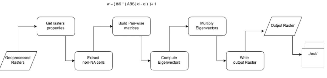
3.2.2. Analytic Hierarchy Process

The process that will be described here, is mentioned in the first paragraph of the

system design chapter, and visible on figure 6. The overview of the flowchart of

this process is illustrated in figure 4.

Figure 4 Flowchart of the AHP computation

Remembering that at this point, we have all data in raster format, and with the

values of the grading scale, see table 4, all rasters were standardized for the AHP

computation. The first step of this process, is to retrieve the raster properties, like

the number of rows and columns, the coordinate reference system, the projection

(35)

26

the computation. Since they fall out of the study region, there is no need to

process these cells. The succeeding step is to compute the pairwise comparison

matrices. These matrices are usually filled by the user, as in most cases there is a

restricted number of alternatives. In this application we are dealing with possibly

around 37 000 alternatives, it becomes almost impossible to pairwise compare all

alternatives. Instead, we use the grading provided by the user, for an automatic

computation of these matrices. This will be explained in detail further down. The

computation of the eigenvectors is the next step. The eigenvectors of the alternatives’ pairwise comparison matrices are computed, as well as, the criteria’s pairwise comparison matrix eigenvector. To better understand the process an

illustration of the process is given, in figure 5.

Figure 5 Detailed flowchart of the AHP system design.

After the eigenvectors are calculated these are multiplied by the eigenvector of the

criteria, see figure 5, resulting into a ranking of the alternatives, the suitability of

each raster cell for the solution of the problem. The ranking is written in a raster

image after the normalization, and this is the final output of the application

(36)

27

As mentioned in the requirements section, one of these requirements was the need

for a big number of alternatives. The idea to solve this was the use of a raster map

where each cell is an alternative. When each cell is a possible alternative then it

becomes almost impossible to pairwise compare all alternatives, since the number

of comparisons is close to the square of the possible alternatives. And we multiply

this number by the number of criteria, plus the number of criteria squared, this

gives us the total number of pairwise comparisons. Which for the Lisbon district,

for example, with a total area of 2800km2, and a 1km by 1km cell size, translates

into 2800 alternatives. Assuming the criteria were only 3, this turns into 7 840 000

pairwise comparisons for 1 criterion. Multiplied by 3 is 23 520 000 pairwise

comparisons of the alternatives, plus the 9 pairwise comparison of the criteria

itself. In the end one would have 3 matrices of 2 800 by 2 800 plus one of 3 by 3

to fill in. Could this be done by hand? Maybe, if filled in randomly, where the

consistency ratio of the matrices would never be under 0.10, the maximum value

accepted (Malczewski, 1999).

To solve this problem the grading scale is used in order to reduce the comparisons

done by the user or decision maker. The scale ranging from 1 to 10, see table 4, is

used to establish priority of the criteria values. This means that instead of

comparing the alternatives with each other according to a specific criteria, the user

will order the possible values of each criterion with the grading scale, and the

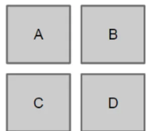
order proposed will always be respected to all alternatives. In case we have 4

alternatives, A, B, C and D, see figure 6, these being raster image cells, and 3

criterion, them being, soil type, slope and population density, the grading tables

being table 7, 8 and 9 respectively.

(37)

28

Table 7 Soil type grading table.

Table 8 Population density grading table.

Table 9 Slope grading table.

Now the real values of the alternatives for the 3 criteria are:

 Soil type:

 A – Sandy

 B – Basalt

 C – Clayey

 D – Water

 Population density:

 A – 11

 B – 8

 C – 2

 D – 0

 Slope

 A – 2%

(38)

29

 C – 1%

 D – 0%

After the reclassification in the geoprocess, the values of A, B, C and D would be

standardized to the same scale, the grading scale, as in table 10.

Alternatives Soil type Population density Slope

A 1 5 10

B 10 8 8

C 8 10 10

D 0 10 10

Table 10 Overall grading table of the alternatives.

From this table the pairwise comparison matrices for each criterion are produced

using the formula below:

(1)

Where,

is one cell of index i, and is the cell with index j that .

are the values of the cells or respectively.

This formula will translate the grading scale values of each cell into a pairwise

comparison value of Saaty’s fundamental scale. Producing the comparison

matrices of the alternatives according to each criterion. This process reduces the

number of comparisons needed, and no matter the number of cells, the number of

grading tables will not change, neither the number of classifications done by the

user.

One problem that erupted from the use of the eigenvectors, is that the eigenvectors

of matrices of 30 000 by 30 000, take too long to compute making the application

software run for hours. So after some research an approximation method was

found to overcome this problem, to substitute the eigenvectors calculation by the

(39)

30

discusses the possibility of substituting the eigenvectors by another less complex

method that would achieve the same results. This research also suggests that the

eigenvalue procedure, is the only one that does not depend on the scale, leads to

the measurements of inconsistency, and is the only procedure that preserves

ranking of the alternatives under inconsistency conditions.

The problem of inconsistency defines that , and presumably if

inconsistency is present in the pairwise comparison matrix, the given comparisons

are questionable and new comparisons may be needed (Saaty & Vargas, 1984).

The consistency however might be tolerated up to 0.1(Malczewski, 1999; Saaty,

2000) Using the example above, A has a sandy soil type, B has a basalt soil type

and C has a clayey soil type. If the grading scale is the same as in table 5 then, A

and all other sandy cells, will always have the value 1 in the grading scale B and

all the other basalt cells will always have the value 10 and C and all clayey cells

will always have the value 8. With this statement one can apply the equation

above to build the comparison matrix of the alternatives A, B and C according to

soil type.

₍₄₎

(5)

(6)

When building the comparison matrix, always a square matrix, we have to

compare the alternatives in pairs according to a specific criterion, in this case soil type. The matrix is built with the values from Saaty’s fundamental scale, see table 1 in the annex. The main diagonal of the matrix will always contain the value 1, according to Saaty’s fundamental scale, the value 1 represents that both activities contribute equally to the objective. Implying, alternative A compared with itself,

will always contribute equally in soil type to the objective. Another fact is that the

matrices are reciprocal e.g. (Saaty, 1987). Suggesting, that when one

compares A with B (A, B) and defines that A is extremely more important for the

(40)

31

opposite comparison (B, A) is 1/9. The matrix below shows the resulting pairwise

comparisons of the automatic grading.

(7)

One problem arose when using equation 1, the result will always be a value from

1 to 9, considering Saaty’s fundamental scale. While sometimes it should be the

reciprocal value. Take the comparison of A with B, equation 4, for example, this

comparison should result in 1/9, and not 9, because B is the alternative with the

best value for the objective. To overcome this problem, the application software

will test which alternative had the highest grading scale value. The one with the highest will get the value of Saaty’s fundamental scale, the lowest one will get the reciprocal, as shown in the Z matrix.

Assuming that the columns and rows of the Z matrix are ordered as A, B and C

respectively the comparison of A against B was 9, but as B had the highest value

in the grading scale the comparison of B against A is the one who gets the value 9

and the comparison A against B will get the reciprocal.

It is said, that for a matrix to be consistent, it should respect the consistency

criterion mentioned above, but please note, that is . The

result should be 3, according to the consistency principle, and 3 is bigger than ,

but then we enter the reciprocal value in of , which is lower than , the

expected value according to the consistency criterion. The importance of this

observation, is that while one value is less than the corresponding consistency

value, the other exceeds it and there is a tendency to compensate. Maintaining the

consistency ratio within acceptable values, lower than 0.10 (Saaty, 1987).

The Logarithmic Least Square Method (LLSM)

Saaty based the AHP in the permissive that organizing paired comparisons in matrixes the underlying ratios α could be found, giving a priorities to the factors being compared. The ratios α of a given matrix

(41)

32

be obtained through the eigenvalue, logarithmic least square or least square

method (Saaty & Vargas, 1984). The one used is the logarithmic least square method, which estimates α through the vector derived by minimizing (8):

(8)

The solution to this minimization problem is given by (9):

₍₉₎

Imposing the condition that the sum of all ranking values is 1, :

(10)

The LLSM as being the most practical, to implement, of the three methods

proposed by Saaty & Vargas (1984), was applied in the application software to

substitute the eigenvalues computation. This method obtains the , ranking