Bioinformatics analyses and approaches to RNA-Seq Data

(1)

2017

FACULDADE DE CIÊNCIAS

DEPARTAMENTO DE BIOLOGIA ANIMAL

Bioinformatics Analyses and Approaches to RNA-Seq Data

Eric Serafim Ramos de Sousa

Mestrado em

Bioinformática

e Biologia Computacional

Especialização em Bioinformática

Dissertação orientada por:

Professor Doutor Octávio S. Paulo

(2)

ii

Acknowledgments

I would like to thank my supervisor at the University of Lisbon, Professor Octávio S. Paulo, for his guidance and advice.

I would also like to thank Dr. João Pedro de Magalhães, for allowing me the opportunity to develop this project in the Integrative Genomics of Ageing Group. He also provided me the guidance and motivation to get this project through the finish line.

I am also grateful to Sipko van Dam for building some of the tools used in this project and for the innumerous hours discussing code and bioinformatics.

To my friends who keep me sane by making me get of my house more, my sincere gratitude, you know who you are.

Finally, to my family, who will never understand what I’ve been studying for all these years but never stopped supporting me, my deepest appreciation.

(3)

iii

Resumo

O envelhecimento ainda é um processo mal compreendido e a identificação dos moduladores mais importantes do envelhecimento continua a ser um desafio. Neste estudo, dados de RNA-Seq de duas experiências diferentes foram analisadas através de técnicas bioinformáticas para tentar encontrar genes nos processos de envelhecimento e antienvelhecimento.

Uma das experiências tinha como intenção comparar o transcriptoma de células de ratinho e de rato-toupeira pelado depois de terem sido stressadas para tentar entender os processos biológicos por trás da resistência do rato-toupeira pelado contra compostos prejudiciais ao ADN. A outra experiência tinha como intenção avaliar as alterações do transcriptoma após o silenciamento do gene Bc055324 em células humanas.

Os dados das experiências foram mapeados contra os genomas de referência usando STAR, as contagens de transcriptos por gene foram obtidas usando o ReadCounter e a expressão diferencial foi explorada usando edgeR. Quando alguns dos resultados pareceram estranhos, a ferramenta FastQ Screen foi usada para tentar entender a origem do problema.

Numa das experiências, o batch effect era muito grande, e mesmo depois de ajustá-lo matematicamente, não permitindo que muitas inferências fossem tiradas. Na outra experiência, um grande erro durante sua execução significou que seu conceito inicial não foi alcançado.

O gene Unc79 é identificado como um gene diferencialmente expresso positivamente ao comparar células de rato-toupeira pelado que foram tratadas com camptotecina após 48 horas contra um controlo. Embora exista um homólogo de ratinho para este gene, não existe expressão nas amostras de ratinho. O gene Unc79 pode então ter um papel importante na resistência do rato-toupeira pelado contra compostos prejudiciais ao ADN.

Este estudo realça a importância de um planeamento e execução adequados das experiências. Apesar do facto de que o custo da sequenciação da NGS estar a diminuir, ainda é uma técnica dispendiosa, e se uma experiência não for executada corretamente pode resultar num desperdício de recursos preciosos. Este estudo também destaca como a Bioinformática é um campo multidisciplinar e que, sem dados de qualidade, mesmo as melhores ferramentas não ajudarão a tirar conclusões sobre uma determinada situação.

Palavras-chave: Bioinformática, Biologia do envelhecimento, RNA-Seq, Rato-toupeira pelado,

(4)

iv

Abstract

Ageing is still a poorly understood process and identifying the most important modulators of ageing remains a challenge. In this study, RNA-Seq data from two different experiments were put through bioinformatics pipelines to try and find genes in ageing and anti-ageing processes.

One of experiments was to compare the transcriptome of naked mole-rat and mouse cells after they’ve been stressed to try to understand the biological processes behind naked mole-rat’s resistance against DNA-damaging agents. The other experiment was to evaluate the alterations of the transcriptome after the silencing of gene Bc055324 in human cells.

Data from the experiments was mapped to reference genomes using STAR, read counts per gene were obtain using ReadCounter and differential expression was explored using edgeR. When some unusual results appeared, FastQ Screen was used to try to understand the source of the problem.

In one of the experiments the batch effect was simply too great, even after adjusting for it mathematically, not allowing for many inferences to be made. On the other experiment, a big mistake during its execution meant that its initial concept was not achieved.

Gene Unc79 is identified as a positively differentially expressed gene when comparing naked mole-rat cells who were treated with campthotecin after 48 hours to control cells. Even though there is a mouse homolog to this gene, there isn’t expression in the mouse samples. Gene Unc79 may be an important player in naked mole-rat’s resistance against DNA-damaging compounds.

This study highlights the importance of proper design and execution of experiments. Even though the cost of NGS sequencing is going down, it is still an expensive technique, if an experiment isn’t properly executed it may result in a waste of precious resources. This study also highlights how Bioinformatics is a multidisciplinary field and that without good data even the best tools won’t help to make conclusions about a certain situation.

(5)

v

Resumo Alargado

Grandes quantidades de informação de origem biológica são produzidas todos os dias e a única maneira de processar toda essa informação é através de técnicas computacionais. É aí que entra a Bioinformática. A Bioinformática poder ser essencialmente dividida em três ramos. O primeiro ramo é a criação e manutenção de bases de dados onde esta informação de origem biológica possa ser guardada, estas bases de dados têm de permitir que os investigadores tenham acesso fácil à informação, mas estas bases de dados também têm de permitir a deposição de mais informação também de uma maneira fácil. O segundo ramo é a criação de algoritmos e programas para analisar a processar a informação de origem biológica. O último ramo é a utilização dos algoritmos e programas para processar a informação guardadas nas bases de dados.

O envelhecimento ainda é um processo mal compreendido e a identificação dos moduladores mais importantes do envelhecimento continua a ser um desafio. Neste estudo, dados de RNA-Seq de duas experiências diferentes foram analisadas através de técnicas bioinformáticas para tentar encontrar genes nos processos de envelhecimento e antienvelhecimento.

A Experiência A tinha como intenção comparar o transcriptoma de células de ratinho e de rato-toupeira pelado depois de terem sido stressadas para tentar entender os processos biológicos por trás da resistência do rato-toupeira pelado contra compostos prejudiciais ao ADN. A Experiência B tinha como intenção avaliar as alterações do transcriptoma após o silenciamento do gene Bc055324 em células humanas.

RNA-Seq é um método de análise do transcriptoma que usa as tecnologias NGS. RNA-Seq é também o método mais preciso para avaliar os níveis de transcritos e suas isoformas.

Os ratos-toupeira pelados tornaram-se parte da pesquisa de envelhecimento quando, em 2002, foi identificado que eles exibiam uma longevidade extraordinária e que eles eram os roedores que viviam até mais tarde. Agora, sabemos que a maioria dos ratos-toupeira pelados vivem geralmente pelo menos 20 anos, com uma vida que pode exceder 31 anos em cativeiro, mais de oito vezes do que ratinhos de tamanho semelhante. Os fibroblastos de rato-toupeira pelado são definitivamente mais resistentes do que os de ratinho a vários metais pesados e compostos prejudiciais ao DNA. Até recentemente, não havia casos documentados de cancro em ratos-toupeira pelados, o que significa que eles têm uma defesa efetiva contra compostos prejudiciais ao DNA e que isso provavelmente contribui para a sua habilidade para atingir uma longevidade extraordinária.

A Experiência A tinha 36 amostras que resultaram em 72 ficheiros fastq files porque as amostras foram sequenciadas usando sequenciação paired-end. Esses 72 ficheiros foram analisados usando FastQC para verificar a sua qualidade. Como eram muitos ficheiros os resultados do FastQC foram compilados usando MultiQC para que a sua visualização fosse mais fácil.

Os ficheiros correspondentes às amostras de ratinho foram depois mapeados contra o genoma de ratinho e os ficheiros correspondentes às amostras de rato-toupeira pelado foram mapeados contra o genoma de rato-toupeira pelado, usando a ferramenta STAR. Mais uma vez como eram muitos ficheiros os resultados do STAR foram compilados usando MultiQC para que a sua visualização fosse mais fácil. As contagens de transcriptos por gene foram obtidas usando o ReadCounter e esses resultados foram analisados usando edgeR.

Os genes onde se verificaram não haver transcritos foram retirados para facilitar a análise e após isso as amostras foram normalizadas. Através de um gráfico de MDS verificou-se que as amostras se agrupavam pelo replicado sugerindo assim que havia um batch effect nos dados. Tentou-se ajustar matematicamente este problema, mas mesmo assim só foi possível identificar o gene Unc79 como um

(6)

vi

gene diferencialmente expresso positivamente ao comparar células de rato-toupeira pelado que foram tratadas com camptotecina após 48 horas contra um controlo. Embora exista um homólogo de ratinho para este gene, não existe expressão nas amostras de ratinho. O gene Unc79 pode então ter um papel importante na resistência do rato-toupeira pelado contra compostos prejudiciais ao ADN.

O procedimento para a Experiência B foi semelhante ao da Experiência A. A Experiência B tinha 12 amostras que resultaram em 24 ficheiros fastq files porque as amostras foram sequenciadas usando sequenciação paired-end. Esses 24 ficheiros foram analisados usando FastQC para verificar a sua qualidade. Como eram muitos ficheiros os resultados do FastQC foram compilados usando MultiQC para que a sua visualização fosse mais fácil.

Os ficheiros foram então mapeados contra o genoma humano usando a ferramenta STAR. Os resultados do STAR foram compilados usando MultiQC para que a sua visualização fosse mais fácil, mas os resultados foram maus sugerindo um problema nas amostras. Como as amostras da Experiência A e da Experiência B foram enviadas para a sequenciação ao mesmo tempo, tentou-se perceber se elas pudessem de alguma maneira estar trocadas. Para isso usou-se a ferramenta FastQ Screen para mapear os ficheiros da Experiência B contra os genomas do ratinho, do rato-toupeira e do humano. Os resultados do FastQ Screen indicaram que todos os ficheiros continham amostras de ratinho. Como todas as amostras da Experiência A não tinham dado problemas conclui-se que o problema não deveria uma troca entre as amostras Experiência A e da Experiência B. O Centre for Genomic Research at the University

of Liverpool, local onde a sequenciação foi feita, foi contactado para perceber se teriam enviado os

resultados errados. A resposta foi que as únicas amostras de ratinho que estavam a sequenciar na altura eram as da Experiência A. Como a hipótese de troca entre a Experiência A e da Experiência B já tinha sido afastada esse não era o problema. Antes da sequenciação verificou-se que duas das amostras continham menos ARN do que as outras e nos ficheiros também se verificou que duas amostras também tinham menos ARN, concluiu-se então que as amostras enviadas para sequenciação eram de ratinho e não de humano indicando assim que a Experiência B tinha sido realizada em células de ratinho em vez de células humanas.

Como o ratinho tem um gene homólogo ao Bc055324 a análise dos resultados prosseguiu. Os ficheiros foram então mapeados ao genoma de ratinho. Os resultados do STAR foram compilados usando MultiQC para que a sua visualização fosse mais fácil.

As contagens de transcriptos por gene foram obtidas usando o ReadCounter e esses resultados foram analisados usando edgeR.

Os genes onde se verificaram não haver transcritos foram retirados para facilitar a análise e após isso as amostras foram normalizadas. Antes da análise de expressão diferencial ter sido realizada, os níveis de expressão do gene BC055324 foram verificados. O que foi verificado foi que havia níveis semelhantes de expressão desse gene em todas as amostras, sugerindo que o silenciamento do gene não tinha funcionado. É compreensível que o silenciamento do gene não funcionado, pois era suposto ser o gene humano e não o gene de ratinho. Uma vez que o silenciamento não funcionou, uma análise mais aprofundada não foi feita, uma vez que não havia mais inferências a fazer no contexto desta experiência. Este estudo realça a importância de um planeamento e execução adequados das experiências. Apesar do facto de que o custo da sequenciação da NGS estar a diminuir, ainda é uma técnica dispendiosa, e se uma experiência não for executada corretamente pode resultar num desperdício de recursos preciosos. Este estudo também destaca como a Bioinformática é um campo multidisciplinar e que, sem dados de qualidade, mesmo as melhores ferramentas não ajudarão a tirar conclusões sobre uma determinada situação.

(7)

vii

Acknowledgments ...ii Resumo ... iii Abstract ... iv Resumo Alargado ... v List of Tables ... ix List of Figures ... x 1 Introduction ... 1 1.1 Ageing ... 1 1.2 RNA-Seq ... 2 1.3 Motivation ... 5 1.4 Objectives ... 6 2 Methods ... 7 2.1 Experiment A ... 7 2.1.1 Quality Control ... 7 2.1.2 Mapping... 7 2.1.3 Differential Expression ... 8 2.2 Experiment B ... 9 2.2.1 Quality Control ... 9 2.2.2 Mapping... 9 2.2.3 Differential Expression ... 10

3 Results and Discussion ... 11

3.1 Experiment A ... 11 3.1.1 Quality Control ... 12 3.1.2 Mapping... 14 3.1.3 Differential Expression ... 16 3.2 Experiment B ... 21 3.2.1 Quality Control ... 21 3.2.2 Mapping... 23 3.2.3 Differential Expression ... 26 4 Conclusions ... 27 4.1 Future Work ... 27 5 References ... 28

(8)

viii

6 Appendix ... 30

6.1 Experiment A ... 30

6.2 Experiment B ... 30

(9)

ix

List of Tables

Table 3.1 Samples from Experiment A and the treatment they were subjected to ... 11

Table 3.2 Results of mapping the samples to the reference genome using STAR ... 14

Table 3.3 Reads uniquely mapped to exons of genes using ReadCounter ... 15

Table 3.4 Normalization factors for the mouse samples ... 16

Table 3.5 Number of differentially expressed genes in the mouse samples for each comparison ... 17

Table 3.6 Normalization factors for the naked mole-rat samples ... 19

Table 3.7 Number of differentially expressed genes in the naked mole-rat samples for each comparison ... 20

Table 3.8 Samples from Experiment B and the treatment they were subjected to ... 21

Table 3.9 Results of mapping the samples to the human reference genome using STAR ... 23

Table 3.10 Results of mapping the samples to the mouse reference genome using STAR ... 24

Table 3.11 Reads uniquely mapped to exons of genes using ReadCounter ... 25

(10)

x

List of Figures

Figure 1.1 20-year-old Naked Mole-rat (Lewis and Buffenstein, 2016) ... 2

Figure 1.2 Advantages of RNA-Seq compared to other transcriptomics methods (Wang et al., 2009) .. 3

Figure 3.1 Mean quality scores across each base position in the read ... 12

Figure 3.2 Per sequence quality scores... 13

Figure 3.3 Per sequence GC Content ... 13

Figure 3.4 MDS plot for the mouse samples ... 17

Figure 3.5 Plot of up and down regulated genes in the 8h Con vs 8h Cam comparison. Only the colored dots are statistically relevant genes ... 18

Figure 3.6 Top 10 mouse genes with the lowest FDR in the 8h Con vs 8h Cam comparison. Above the top 10 genes before the adjustment to the design matrix. Below the top 10 genes after the adjustment. ... 18

Figure 3.7 MDS plot for the naked mole-rat samples ... 19

Figure 3.8 Top 10 naked mole-rat genes with the lowest FDR in the 48h Con vs 48h Cam comparison. Above the top 10 genes before the adjustment to the design matrix. Below the top 10 genes after the adjustment. ... 20

Figure 3.9 Mean quality scores across each base position in the read ... 21

Figure 3.10 Per sequence quality scores... 22

Figure 3.11 Per sequence GC Content ... 22

Figure 3.12 FastQ Screen results for file 1 of Sample R148CO ... 23

Figure 3.14 MDS plot for the samples from Experiment B ... 26

Figure 6.11 FastQ Screen results for file 1 of Sample R148BC... 34

(11)

1

1 Introduction

1.1 Ageing

Ageing can simply be defined as a progressive deterioration of physiological function, accompanied by an increase in vulnerability and mortality with age (de Magalhães, 2011). The initial views of ageing assumed that all deaths are attributable to either evident or hidden disease, making then the assumption that the elimination of disease would result in an increase in life expectancy. This is basically what occurred in the 20th century, many people then concluded that this model of ageing was correct. But during the last half of the century, another point of view arose, which disputed this older interpretation, the main evidence for the disagreement was the observation that the increased life span in the 20th century involved an increase in the mean life span but not in the maximum life span and that even healthy and disease-free organisms aged. Backed up by experimental data, the conclusion was that ageing is not the outcome of disease or pathological processes, but rather results from the evolutionary tendency of organisms to allocate more energy to reproduction than to preservation (Arking, 2006).

To understand ageing we must then account for the intrinsic complexity of biological systems (de Magalhães, 2011). Ageing increases the probability with time that the individual will die while also decreasing the ability of an individual to withstand extrinsic stresses (Arking, 2006). Ageing likely involves multiple processes and possibly the interplay between various causal mechanisms (de Magalhães and Tacutu, 2016), hundreds of genes have been associated with ageing in model organisms (Tacutu et al., 2013), and yet the pathways involved are complex and often interact in nonlinear ways (de Magalhães et al., 2012).

Is ageing then a universal biological trait? There is some evidence suggesting that ageing as we have defined it occurs in at least some bacterial species, but strong and broad evidence of aging is found only among eukaryotes (Arking, 2006).

There is no consensus on what the driving force of ageing is or what type of components play a role in it, which makes it nearly impossible to model ageing in higher organisms with precision (de Magalhães, 2009). Ageing is so highly individual that average curves give only a rough approximation of the pattern of ageing followed by individuals. Knowing that a certain individual has a quantifiable decrease in a physiological function may or may not be a sufficient basis for saying anything reliable about that individual’s rate of ageing, much less predicting his or her longevity (Arking, 2006).

Ageing and longevity are two concepts inherently related. Longevity is defined as the maximum lifespan for an individual or, for species, it is determined by the age until which the great majority of individuals live (Butler and Jasmin, 2000). Although there are several similarities between ageing and longevity, genes associated with longevity are not always involved in the ageing process (de Magalhães, 2009). Longevity, as ageing, is still poorly understood so some of the more recent studies in longevity research have focused in the prediction of longevity candidate genes using human orthologues (Tacutu

et al., 2012).

Naked mole-rats are highly social, rodents naturally found in the hot, arid regions of the north-eastern Horn of Africa where they lead a strictly subterranean existence. These buck-toothed, furless mammals look like miniature walruses but they have a translucent, wrinkled and essentially hairless pink skin (Lewis and Buffenstein, 2016).

(12)

2

Figure 1.1 20-year-old Naked Mole-rat (Lewis and Buffenstein, 2016)

Naked mole-rats became a part of ageing research when, in 2002, it was reported that they exhibited extraordinary longevity and that they were the longest-lived rodents documented. Now we know that most naked mole-rats usually live to at least 20 years (Figure 1.1), with a lifespan that can exceed 31 years in captivity, more than eight times longer than similar-sized mice. Naked mole-rat fibroblasts are markedly more resistant than those of mice, to various heavy metals including cadmium, chromium, and zinc, heat stress, the oxidative stressor paraquat, DNA-damaging compounds including adriamycin, camptothecin, and methyl methanesulfate (MMS), and low-glucose stress (Lewis and Buffenstein, 2016). Until recently there were no documented cases of cancer in naked mole-rats (Delaney et al., 2016), this means that naked mole-rats have an effective defence against DNA-damaging agents and that this likely contributes to their delayed and decreased ageing profile and affiliated ability to attain extraordinary longevity (Lewis and Buffenstein, 2016).

In order to find out which genes are active in a particular cell type and what might make that cell different, studying the RNA that is transcribed from these genes, bring us closer to understanding how a cell can perform its specialized job. In addition to comparing the expressed genes between different types of cells, we can also study how these patterns of gene expression change over time or in response to different stimuli. One of the best techniques to do that kind of study is RNA-Seq (Kukurba and Montgomery, 2016).

1.2 RNA-Seq

RNA-Seq is an approach to transcriptome profiling that uses NGS technologies. RNA-Seq also provides a far more precise measurement of levels of transcripts and their isoforms than other methods (Kukurba and Montgomery, 2016).

The transcriptome is the complete set of transcripts in a cell and their concentration for a specific developmental stage or physiological condition. Understanding the transcriptome is essential for interpreting the functional elements of the genome and revealing the molecular constituents of cells and tissues, and for understanding development and disease. The key aims of transcriptomics are: to catalogue all species of transcript, to determine the transcriptional structure of genes and to quantify the changing expression levels of each transcript during development and under different conditions (Wang

et al., 2009).

The previous methods to quantify the transcriptome present several limitations going from reliance upon existing knowledge about genome sequence, high background levels owing to cross-hybridization and a limited dynamic range of detection owing to both background and saturation of signals. Not only that, comparing expression levels across different experiments is often difficult and can require complicated normalization methods (Wang et al., 2009).

RNA-Seq works by converting population of RNA to a library of cDNA fragments with adaptors attached to one or both ends (single-end vs paired-end sequencing). Each molecule, with or without amplification, is then sequenced in a high-throughput manner to obtain short sequences of varying lengths depending on the technology. Following sequencing, the resulting reads are either aligned to a reference genome or reference transcripts, or assembled de novo without the genomic sequence to

(13)

3

produce a genome-scale transcription map that consists of both the transcriptional structure and/or level of expression for each gene (Wang et al., 2009).

RNA-Seq presents various advantages over previous technologies (Figure 1.2), unlike hybridization-based approaches, it is not limited to detecting transcripts that correspond to existing genomic sequences. This makes RNA-Seq particularly useful for non-model organisms with genomic sequences that are yet to be determined. RNA-Seq can reveal the precise location of transcription boundaries, to a single base resolution allowing for the detection of sequence variations like SNPs. It also gives information about how two exons are connected which can reveal connectivity between multiple exons. RNA-Seq has very low, background signal because DNA sequences can be unambiguously mapped to unique regions of the genome. RNA-Seq has a large dynamic range of expression levels over which transcripts can be detected contrasting with DNA microarrays which lack sensitivity for genes expressed either at low or very high levels. RNA-Seq has also been shown to be highly accurate for quantifying expression levels, as determined using quantitative PCR. The results of RNA-Seq also show high levels of reproducibility, and because there are no cloning steps it requires less RNA sample. RNA-Seq is the first sequencing based method that allows the entire transcriptome to be surveyed in a very high-throughput and quantitative manner with a relative low cost (Wang et al., 2009).

Figure 1.2 Advantages of RNA-Seq compared to other transcriptomics methods (Wang et al., 2009)

As expected, RNA-Seq does not come without it’s challenges, although there are only a few steps in RNA-Seq, it does involve several manipulation stages during the production of cDNA libraries, which can complicate its use in profiling all types of transcript, larger RNA molecules must be fragmented into smaller pieces to be compatible with most deep-sequencing technologies creating a bias in the outcome depending on the method used for fragmentation. Some steps during library construction can also complicate the analysis of RNA-Seq, there could be PCR artefacts or artefacts of reverse transcription if it has been chosen to use strand-specific libraries (Wang et al., 2009).

Bioinformatics is key to making the most out of RNA-Seq. For starters, pre-processing is necessary to remove low-quality reads.

FastQC is a tool that provides a quality control report that can identify problems that originate in the sequencer or in the library material. This step is a simple way to perform some quality control checks to ensure that the raw data looks acceptable and that there are no problems that may affect the analysis

(14)

4

of the data. FastQC can be run as a standalone interactive application for the immediate analysis of small numbers of fastq files or it can be run on a command line in order to allow the processing of a large number of files (Andrews, 2010).

MultiQC is a tool that creates a single report visualising output from multiple tools across many samples, enabling global trends and biases to be quickly identified. MultiQC can plot data from many common bioinformatics tools and is built to allow easy extension and customization. Most bioinformatics programs create logs detailing their results, however, nearly all these logs and reports are produced on a per-sample basis, requiring the user to find and compile the results. This is a process that is time consuming, repetitive and complex, making it prone to errors. MultiQC addresses this by scanning given analysis directories for log files, creating a single summary report visualizing results across all samples. By having a single report, it provides a fast way to scan key statistics quickly and shared plots allow accurate comparison between samples, allowing detection of subtle differences not noticeable when switching between different files. MultiQC is the first tool of its type in Bioinformatics and has the potential to greatly improve life for researchers involved in next-generation sequencing, removing the need for custom comparative scripts (Ewels et al., 2016).

Once high-quality reads have been obtained, the first thing to do is to map the short reads from RNA-Seq to the reference genome, or to assemble them into contigs before aligning them to the genomic sequence to reveal transcription structure. However, short transcriptomic reads also contain reads that span exon junctions or that contain poly(A) ends. For large transcriptomes, alignments are also complicated by the fact that a significant portion of sequence reads match multiple locations in the genome. One solution is to assign these multi-matched reads by proportionally assigning them based on the number of reads mapped to their neighbouring unique sequences. This method has been successful for low-copy repetitive sequences. Short reads that have high copy numbers (>100) and long stretches of repetitive regions present a greater challenge. Alternatively, a paired-end sequencing strategy, in which short sequences are determined from both ends of a DNA fragment, extends the mapped fragment length to 200–500 contributing to less repetitive sequences (Wang et al., 2009).

STAR is a tool based on a RNA-Seq alignment algorithm that uses sequential maximum mappable seed search in uncompressed suffix arrays followed by seed clustering and stitching procedure. STAR is capable of running parallel threads on multicore systems with close to linear scaling of productivity with the number of cores, outperforming other aligners in mapping speed. Not only is it faster, it also shows better alignment precision and sensitivity than other RNA-Seq aligners for both experimental and simulated data. In addition to unbiased de-novo detection of canonical junctions, STAR can discover non-canonical splices and chimeric transcripts, and is also capable of mapping full-length RNA sequences. STAR is not an extension of a short-read DNA mapper, like many other RNA-Seq mappers, but was developed as a stand-alone C++ program (Dobin et al., 2013).

ReadCounter is a custom software developed at the Integrative Genomics of Ageing Group at the University of Liverpool to determine read counts per gene. It was developed to substitute the widely used HTseq tool. ReadCounter is more efficient running approximately 3-fold faster on a single core while also utilizing multithreaded technology which results in a 15 to 20 fold faster runtime on an eight core system. ReadCounter automatically counts the number of reads mapping to introns. ReadCounter is written in Java and can be run using a command line in the terminal or command prompt (Mac/Linux/Windows) without the requirement for installation (van Dam et al., 2015). The tool is free to use and publicly available at http://www.genefriends.org/ReadCounter.

Another issue to consider is sequence coverage, or the percentage of transcripts measured, which has implications for cost. Greater coverage requires more sequencing depth. Analysing many different conditions can further increase the coverage and to detect a rare transcript or variant, considerable depth is needed. In general, the larger the genome, the more complex the transcriptome, the more sequencing depth is required for adequate coverage. It is less straightforward to calculate the coverage of the

(15)

5

transcriptome than it is in genome sequencing, this is because the true number and level of different transcript isoforms is not usually known and because transcription activity varies greatly across the genome (Wang et al., 2009).

EdgeR, which is referenced in the literature as the best methodology for differential expression studies (Rapaport et al., 2013; Soneson and Delorenzi, 2013; Zhou et al., 2014; Zhang et al., 2014; Gierliński et al., 2015; Finotello and Di Camillo, 2015; Holik et al., 2016; Schurch et al., 2016), is a Bioconductor software package used for examining differential expression of replicated count data. An over dispersed Poisson model is used to account for both biological and technical variability. Empirical Bayes methods are used to moderate the degree of over dispersion across transcripts, improving the reliability of inference. The methodology can be used even with the most minimal levels of replication, provided at least one phenotype or experimental condition is replicated (Robinson et al., 2009).

There has been no clear consensus on the appropriate normalization method to be used or the impact of a chosen method on the downstream analysis (Dillies et al., 2013). EdgeR is a versatile tool that allows the data to be normalized using your preferred method beforehand or by using its built-in method which is trimmed mean of M-values normalization. The trimmed mean of M-values method estimates scale factors between samples while accounting for the fact that some extremely differentially expressed genes would impact negatively the normalization procedure. (Robinson and Oshlack, 2010). EdgeR can detect differential expression in very different types of experimental conditions either through the generalized linear model likelihood ratio test or the quasi-likelihood F-test. In summary differential expression analysis is just statistical testing to decide whether a gene has a difference in read counts that is greater than what would be expected just due to natural random variation (Oshlack et al., 2010).

The intention of a MDS plot is to project n-dimensional data points to a 2-dimensional space in a manner that similar points in the n-dimensional space will project to near distances in a plane, in other words it is projecting a multidimensional space preserving the inter point distances, employing distance and a loss function to analyse the proximities of data points, while in PCA you project a multidimensional space to the directions of maximum variability using covariance/correlation matrix to analyse the correlation between data points and variables (Hout and Goldinger, 2014).

FastQ Screen is a simple application which allows you to search a large sequence dataset against a panel of different genomes to determine from where the sequences in your data originate. It was built as a quality control check for sequencing pipelines but may also be useful in characterizing metagenomic samples. Although the program wasn't built with any particular technology in mind, it is probably only suitable for processing short reads due to the use of either Bowtie, Bowtie2 or BWA as the searching application. The program generates both text and graphical output to inform you what proportion of your library mapped, either uniquely or to more than one location, against each of your specified reference genomes. The user should then be able to identify a clean sequencing experiment in which the overwhelming majority of reads are probably derived from a single genomic origin (Wingett, 2011).

1.3 Motivation

Ageing is still a poorly understood process and identifying the most important modulators of ageing remains a challenge. Given the intrinsic costs of performing animal ageing studies, developing predictive computational tools is of utmost importance and the accuracy and specificity of current predictive in silico methods is still very limited. In this study, RNA-Seq data from two different experiments will be exploited to develop computational approaches to make testable predictions about

(16)

6

genes in ageing and anti-ageing processes. Because RNA-Seq is a relatively new technique, standard methods for RNA-Seq data analysis are still being discussed and created. Researchers planning experiments need to carefully balance the advantages of the latest next-generation sequencing platforms.

1.4 Objectives

One of the ideas behind Experiment A (Appendix 6.1) was to compare the transcriptome of naked mole-rat and mouse cells after they’ve been stressed to try to understand the biological processes behind naked mole-rat’s resistance against DNA-damaging agents.

The intention of Experiment B (Appendix 6.2) was to evaluate the alterations of the transcriptome after the silencing of gene Bc055324 in human cells. There is evidence that gene Bc055324 might play a role in cancer development (van Dam et al., 2012).

This study will help establish approaches suitable to guide transcriptome sequencing driven studies while also identifying differentially expressed genes in both these sets of data and to try to understand the role that those genes might play through functional enrichment analysis.

(17)

7

2 Methods

This complete analysis was done on a laptop with an Intel Core i7-4700MQ CPU with 8 Gb of RAM memory running Windows 10 Version 1703 and on a 24-core server with 48 Gb of RAM memory running Ubuntu 12.04 LTS Precise Pangolin.

2.1 Experiment A

2.1.1 Quality Control

The sequencing of the 36 samples (Table 3.1) resulted in 72 fastq files because the sequencing was done using paired-end sequencing. Those 72 files were run through FastQC version 0.11.5, to check the quality of the sequencing, producing 72 reports.

Since the number of reports was large, the reports were compiled using MultiQC version 1.2 to make visualization easier.

Both FastQC and MultiQC only have one function and don’t have any parameters to set their function, it is just required to execute the program and indicate the path to the files you want to be analysed. After all the fastq files were put through FastQC and the reports were compiled with MultiQC, no further pre-processing was done because the files showed good quality (Figure 3.1 - Figure 3.3).

2.1.2 Mapping

All fastq files were then mapped to the reference genome using STAR version 2.3.0e r291. The mouse samples were mapped to the mouse genome and the naked mole-rat samples were mapped to the naked mole-rat genome. The mouse genome and annotation used was version GRCm38 from Ensembl release 76 (Cunningham et al., 2015) which were downloaded from the Ensembl ftp server and the naked mole-rat genome and annotation used was HetGla_female_1.0 assembly which was from RefSeq release 67 (O’Leary et al., 2016) which were downloaded from the RefSeq ftp server.

Before the mapping of the samples to the respective genomes, it is first necessary to build a STAR genome index file. In this case, two STAR genome index files were built, one for the mouse genome and one for the naked mole-rat genome. The same STAR parameters were used for both those files. Those parameters were: “--runMode genomeGenerate” this first parameter is used to define the type of function you want STAR to execute, “--genomeDir” this second parameter was followed by the path of where to create index file, “--genomeFastaFiles” this third parameter was followed by the path of the genome file, sjdbGTFfile” this fourth parameter was followed by the path to the annotation file, “--sjdbOverhang 100” this fifth parameter was used to define the length of the donor/acceptor sequence on each side of splice junctions, ideally the value of this number should be read length minus 1, but it is common to use 100 as a safe generic value, “--runThreadN 8” this sixth parameter is used to define how many computer threads STAR should use, the value 8 was chosen because the server where STAR was used had various other users and hogging all of the server’s resources was not desirable.

After having the index files, the mapping was done using the same parameters for both the mouse samples and the naked mole-rat samples. The STAR parameters were: “--genomeDir” this first parameter was followed by the path to the index file (the mouse one for the mouse samples and the naked mole-rat one for the naked mole-rat samples), “--readFilesIn” this second parameter was followed

(18)

8

by the location of the sample files, since the sequencing was paired-end, each sample had two files in this parameter, “ –outFilterMultimapNmax 1” this third parameter with the value 1 simply reports only uniquely mapping reads, “--outSAMstrandField intronMotif” this fourth parameter is to add XS strand tags to spliced reads to help the quality of the assembly, “--sjdbGTFfile” this fifth parameter was followed by the path to the annotation file, “--outFileNamePrefix” this sixth parameter is followed by the name we want to name the files produced by STAR, “--runThreadN 8” this seventh parameter, as before, is used to define how many computer threads STAR should use. Since the number of samples was high and this would be a lengthy process, an AWK script (https://github.com/oldguyeric/mastersthesis/blob/master/domappings.awk) was developed to automate the process of mapping all samples to the genomes.

The alignment resulted in 36 sam files plus 36 log files containing alignment statistics. The logs were compiled using MultiQC to make visualization easier.

Read counts per gene were then determined using ReadCounter version 1.1.1. Not all reads that were mapped using STAR map uniquely to exons of genes. Using ReadCounter we obtain read counts per gene that were uniquely mapped to exons of genes (Table 3.3). The same parameters were used for both the mouse samples and the naked mole-rat samples and they were: “inputFile=” this first parameter was followed by the path to the sam files produced by STAR, “annotation=” the second parameter was followed by the path to the annotation file, “nThreads=8” this third parameter used to define how many computer threads ReadCounter should use.

Since the number of samples was high and this would be a lengthy process, an AWK script (https://github.com/oldguyeric/mastersthesis/blob/master/doreadcounter.awk) was developed to automate the process of generating the read count files.

2.1.3 Differential Expression

Read count information from all the samples was then compiled and processed using edgeR version 3.20.0 on R version 3.4.1 through a R script following the indications from the edgeR user guide, one for the naked mole-rat samples (https://github.com/oldguyeric/mastersthesis/blob/master/nmr.R) and another for the mouse samples (https://github.com/oldguyeric/mastersthesis/blob/master/mouse.R).

The mouse samples and the naked mole-rat samples were handled separately. For the mouse samples, the genes with very low counts across libraries were removed because they provide little evidence for differential expression and may interfere with some of the statistical approximations used later on. This reduced the number of analysed genes from 41388 to 13440. To account for compositional biases, the read counts were normalized using the built-in trimmed mean of M-values normalization method (Table 3.4). One of the ways to do comparisons on edge R is through a design matrix.

To check for similarities between the samples, the data was plotted using a multi-dimensional scaling plot (Figure 3.4). Distances on a MDS plot correspond to leading log-fold-change between each pair of samples. Leading log-fold-change is the root-mean-square average of the largest log2

-fold-changes between each pair of samples. Samples from the same replicate cluster together suggesting that there is a batch effect in the data which needs to be accounted for. The design matrix was then changed to account for the batch effect.

Each gene was tested for significant differential expression using the quasi-likelihood F-test. The quasi-likelihood F-test is preferred as it reflects the uncertainty in estimating the dispersion for each gene. It provides more robust and reliable error rate control when the number of replicates is small. The tests can be viewed as analogous to paired t-tests. All genes were tested against a standard false discovery rate of 0.05. Several comparisons between the experimental conditions were made (Table 3.5).

(19)

9

The procedure for the naked mole-rat samples was the same as the one for the mouse samples. The genes with very low counts across libraries were removed reducing the number of analysed genes from 30562 to 14928. Read-counts were also normalized to account for compositional biases (Table 3.6).

The data was plotted using a multi-dimensional scaling plot (Figure 3.7), and once again the samples from the same replicate cluster together, even more strongly in this case, suggesting that there is a batch effect in the data which needs to be accounted for.

Each gene was tested for signiﬁcant diﬀerential expression using the quasi-likelihood F-test. All genes were tested against a standard false discovery rate of 0.05. Several comparisons between the experimental conditions were made (Table 3.7).

2.2 Experiment B

2.2.1 Quality Control

The sequencing of the 12 samples (Table 3.8) resulted in 24 fastq files because the sequencing was done using paired-end sequencing. Those 24 files were run through FastQC version 0.11.5, to check the quality of the sequencing, producing 24 reports.

Since the number of reports was large, the reports were compiled using MultiQC version 1.2 to make visualization easier.

2.2.2 Mapping

All fastq files were then mapped to the reference genome using STAR version 2.3.0e r291, the samples were mapped to the human genome. The human genome and annotation used was version GRCh38 from Ensembl release 76 which were downloaded from the Ensembl ftp server. The STAR parameters used were similar than those in section 2.1.2 and an AWK script was also made to automate the mapping process (https://github.com/oldguyeric/mastersthesis/blob/master/domappings2.awk).

The alignment resulted in 12 sam files plus 12 log files containing alignment statistics. The logs were compiled using MultiQC to make visualization easier. The results from mapping the samples to the human reference genome using STAR indicate that there might be a problem with the samples (Table 3.8).

The first assumption made was maybe that since the sequencing for Experiment A was sent to sequencing at the same time as Experiment B there might I’ve been a mix up of samples. To evaluate this theory the samples were mapped simultaneously to the human, mouse and naked mole-rat using FastQ Screen.

FastQ Screen version 0.11.1 was used to screen the fastq files against the human genome and annotation version GRCh38 from Ensembl release 76 which were downloaded from the Ensembl ftp server, mouse genome and annotation version GRCm38 from Ensembl release 76 which were downloaded from Ensembl ftp server and the naked mole-rat genome and annotation used was HetGla_female_1.0 assembly which was downloaded from RefSeq release 67 which were downloaded from the RefSeq ftp server, to check if the composition of the samples matched with what was expected. In this case FastQ Screen was used with Bowtie2 version 2.3.2. Bowtie 2 uses a full-text minute index–based approach to permit gapped alignment by dividing the algorithm broadly into two stages: an initial, ungapped seed-finding stage that benefits from the speed and memory efficiency of the full-text minute index and a gapped extension stage that uses dynamic programming and benefits from the

(20)

10

efficiency of single-instruction multiple-data parallel processing available on modern processors (Langmead and Salzberg, 2012). Bowtie 2 human and mouse index files are publicly available at the Bowtie 2 website so had not to be built. The naked mole-rat genome index file was then built using the Bowtie 2 default parameters to build an index.

FastQ Screen doesn’t have parameters but instead uses a configuration file to define what to do. The configuration file (https://github.com/oldguyeric/mastersthesis/blob/master/fastq_screen.conf) was modified to define that Bowtie 2 was the aligner, what the path to genome index files were and how many threads to use.

For reasons explained in section 3.2.2 the samples were also mapped to the mouse genome and annotation version GRCm38 from Ensembl release 76 using STAR. The parameters used were the same as before and once again an AWK script was developed to automate the mapping of all samples (https://github.com/oldguyeric/mastersthesis/blob/master/domappings3.awk). The alignment resulted in 12 sam files plus 12 log files containing alignment statistics. The logs were compiled using MultiQC to make visualization easier. Read counts per gene were then determined using ReadCounter. The parameters for ReadCounter were the same used in section 2.1.2 and an AWK script was developed to automate the process (https://github.com/oldguyeric/mastersthesis/blob/master/doreadcounter2.awk).

2.2.3 Differential Expression

ReadCounter produces tab separated text files with the read counts per gene results. Read count information from all the samples was then compiled and processed using edgeR version 3.20.0 on R version 3.4.1 through a R script (https://github.com/oldguyeric/mastersthesis/blob/master/b.R) following the indications from the edgeR user guide.

The genes with very low counts across libraries were removed because they provide little evidence for differential expression and may interfere with some of the statistical approximations used later on. This reduced the number of analysed genes from 41388 to 14338. To account for compositional biases, the read counts were normalized using the built-in trimmed mean of M-values normalization method (Table 3.12).

The data was plotted using a multi-dimensional scaling plot to check if the batch effect present on the data from Experiment A was an artefact from the pipeline used.

(21)

11

3 Results and Discussion

3.1 Experiment

A

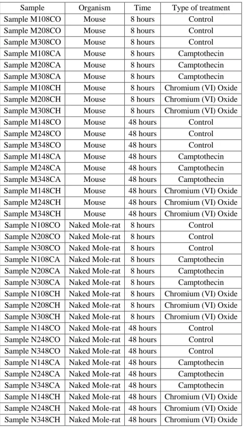
Table 3.1 Samples from Experiment A and the treatment they were subjected to

Sample Organism Time Type of treatment Sample M108CO Mouse 8 hours Control Sample M208CO Mouse 8 hours Control Sample M308CO Mouse 8 hours Control Sample M108CA Mouse 8 hours Camptothecin Sample M208CA Mouse 8 hours Camptothecin Sample M308CA Mouse 8 hours Camptothecin Sample M108CH Mouse 8 hours Chromium (VI) Oxide Sample M208CH Mouse 8 hours Chromium (VI) Oxide Sample M308CH Mouse 8 hours Chromium (VI) Oxide Sample M148CO Mouse 48 hours Control Sample M248CO Mouse 48 hours Control Sample M348CO Mouse 48 hours Control Sample M148CA Mouse 48 hours Camptothecin Sample M248CA Mouse 48 hours Camptothecin Sample M348CA Mouse 48 hours Camptothecin Sample M148CH Mouse 48 hours Chromium (VI) Oxide Sample M248CH Mouse 48 hours Chromium (VI) Oxide Sample M348CH Mouse 48 hours Chromium (VI) Oxide Sample N108CO Naked Mole-rat 8 hours Control Sample N208CO Naked Mole-rat 8 hours Control Sample N308CO Naked Mole-rat 8 hours Control Sample N108CA Naked Mole-rat 8 hours Camptothecin Sample N208CA Naked Mole-rat 8 hours Camptothecin Sample N308CA Naked Mole-rat 8 hours Camptothecin Sample N108CH Naked Mole-rat 8 hours Chromium (VI) Oxide Sample N208CH Naked Mole-rat 8 hours Chromium (VI) Oxide Sample N308CH Naked Mole-rat 8 hours Chromium (VI) Oxide Sample N148CO Naked Mole-rat 48 hours Control Sample N248CO Naked Mole-rat 48 hours Control Sample N348CO Naked Mole-rat 48 hours Control Sample N148CA Naked Mole-rat 48 hours Camptothecin Sample N248CA Naked Mole-rat 48 hours Camptothecin Sample N348CA Naked Mole-rat 48 hours Camptothecin Sample N148CH Naked Mole-rat 48 hours Chromium (VI) Oxide Sample N248CH Naked Mole-rat 48 hours Chromium (VI) Oxide Sample N348CH Naked Mole-rat 48 hours Chromium (VI) Oxide

(22)

12

3.1.1 Quality Control

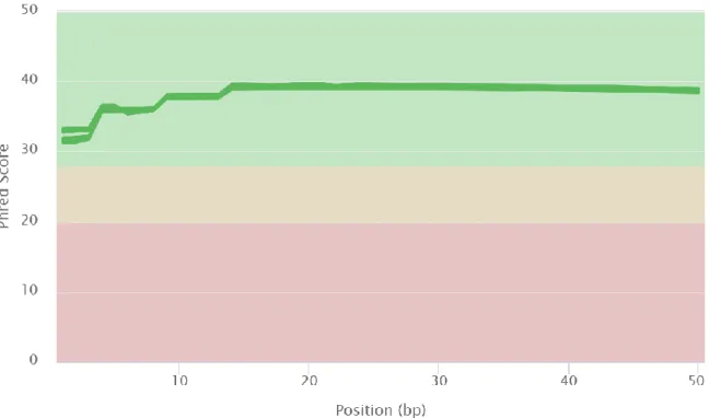
All files have very similar quality scores and that is why it looks like there is only one file in the graph (Figure 3.1) but, in reality, all 72 files are shown. All files show a mean quality Phred score over 30 across the length of the reads (Figure 3.1). Phred quality scores are assigned to each nucleotide base call in automated sequencer traces. A Phred quality score of 30 means there is a base call accuracy of 99.9% and across most of the length of the reads there is a mean quality Phred score of around 40 meaning there is a base call accuracy of 99.99%.

Figure 3.1 Mean quality scores across each base position in the read

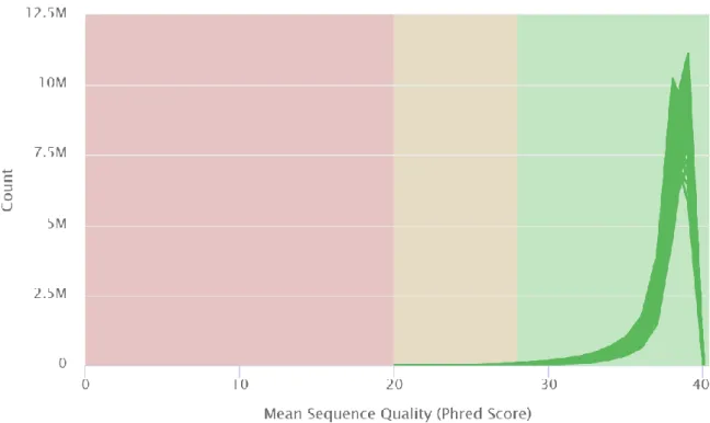
Looking at the files by the quality scores per sequence (Figure 3.2) we can see that once again all files have very similar scores that kind of blob together in the graph, but we can clearly see that all the files have close to ten million reads with Phred scores near 40, showing that there is quality in the sequencing.

(23)

13

Figure 3.2 Per sequence quality scores

The GC content in the files is less uniform (Figure 3.3) than it was for the quality scores, nevertheless, a normal random library typically has a roughly normal distribution of GC content and we can see, even though there is some deviation, all files present a distribution similar to a normal distribution.

(24)

14

3.1.2 Mapping

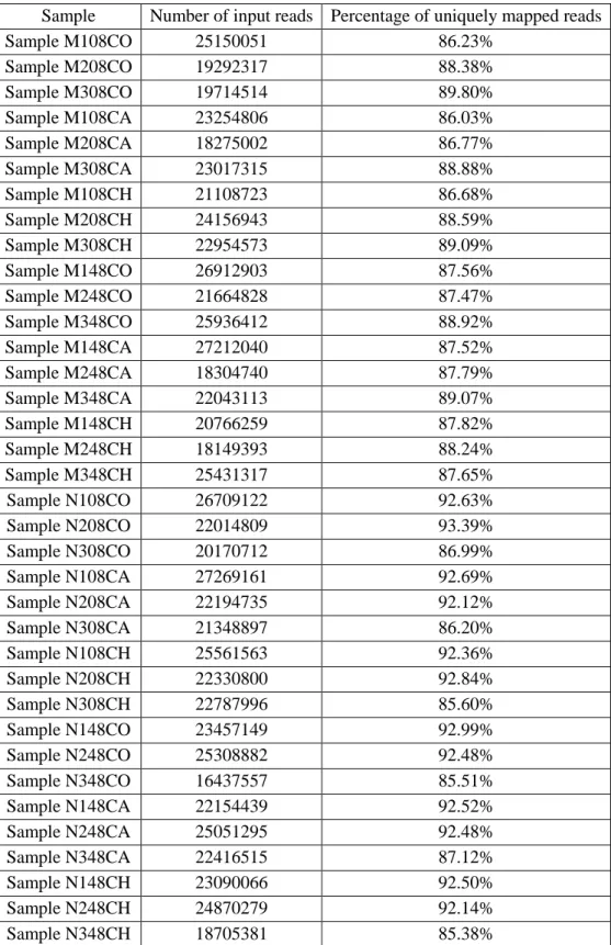
The results from mapping the samples to the reference genomes using STAR resulted in all the samples having a percentage of uniquely mapped reads above 85% (Table 3.2) which is very good.

Table 3.2 Results of mapping the samples to the reference genome using STAR

Sample Number of input reads Percentage of uniquely mapped reads Sample M108CO 25150051 86.23% Sample M208CO 19292317 88.38% Sample M308CO 19714514 89.80% Sample M108CA 23254806 86.03% Sample M208CA 18275002 86.77% Sample M308CA 23017315 88.88% Sample M108CH 21108723 86.68% Sample M208CH 24156943 88.59% Sample M308CH 22954573 89.09% Sample M148CO 26912903 87.56% Sample M248CO 21664828 87.47% Sample M348CO 25936412 88.92% Sample M148CA 27212040 87.52% Sample M248CA 18304740 87.79% Sample M348CA 22043113 89.07% Sample M148CH 20766259 87.82% Sample M248CH 18149393 88.24% Sample M348CH 25431317 87.65% Sample N108CO 26709122 92.63% Sample N208CO 22014809 93.39% Sample N308CO 20170712 86.99% Sample N108CA 27269161 92.69% Sample N208CA 22194735 92.12% Sample N308CA 21348897 86.20% Sample N108CH 25561563 92.36% Sample N208CH 22330800 92.84% Sample N308CH 22787996 85.60% Sample N148CO 23457149 92.99% Sample N248CO 25308882 92.48% Sample N348CO 16437557 85.51% Sample N148CA 22154439 92.52% Sample N248CA 25051295 92.48% Sample N348CA 22416515 87.12% Sample N148CH 23090066 92.50% Sample N248CH 24870279 92.14% Sample N348CH 18705381 85.38%

(25)

15

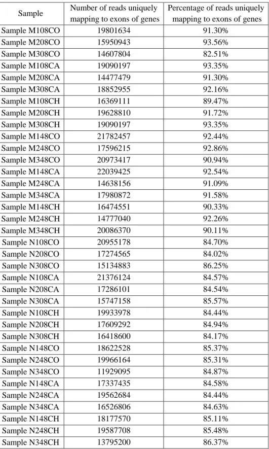
Not all reads that were mapped using STAR map uniquely to exons of genes. Using ReadCounter we obtain read counts per gene that were uniquely mapped to exons of genes (Table 3.3). The resulting reads are the ones which are going to be analysed for differential expression.

Table 3.3 Reads uniquely mapped to exons of genes using ReadCounter

Sample Number of reads uniquely mapping to exons of genes

Percentage of reads uniquely mapping to exons of genes Sample M108CO 19801634 91.30% Sample M208CO 15950943 93.56% Sample M308CO 14607804 82.51% Sample M108CA 19090197 93.35% Sample M208CA 14477479 91.30% Sample M308CA 18852955 92.16% Sample M108CH 16369111 89.47% Sample M208CH 19628810 91.72% Sample M308CH 19090197 93.35% Sample M148CO 21782457 92.44% Sample M248CO 17596215 92.86% Sample M348CO 20973417 90.94% Sample M148CA 22039425 92.54% Sample M248CA 14638156 91.09% Sample M348CA 17980872 91.58% Sample M148CH 16474551 90.33% Sample M248CH 14777040 92.26% Sample M348CH 20086370 90.11% Sample N108CO 20955178 84.70% Sample N208CO 17274565 84.02% Sample N308CO 15134883 86.25% Sample N108CA 21376124 84.57% Sample N208CA 17286101 84.54% Sample N308CA 15747158 85.57% Sample N108CH 19933978 84.44% Sample N208CH 17609292 84.94% Sample N308CH 16418600 84.17% Sample N148CO 18622528 85.37% Sample N248CO 19966164 85.31% Sample N348CO 11929095 84.87% Sample N148CA 17337435 84.58% Sample N248CA 19562684 84.44% Sample N348CA 16526806 84.63% Sample N148CH 18177570 85.11% Sample N248CH 19587708 85.48% Sample N348CH 13795200 86.37%

(26)

16

3.1.3 Differential Expression

Table 3.4 Normalization factors for the mouse samples

Sample Library Size Normalization Factor Sample M108CO 19777810 0.9969735 Sample M208CO 15936960 0.9646242 Sample M308CO 14579716 1.0377587 Sample M108CA 18384278 1.0006793 Sample M208CA 14461040 1.0358069 Sample M308CA 18830698 0.9897061 Sample M108CH 16340570 0.9357663 Sample M208CH 19607263 0.9882831 Sample M308CH 19070108 0.9639682 Sample M148CO 21758296 1.0323033 Sample M248CO 17580451 0.9607669 Sample M348CO 20947466 0.9883213 Sample M148CA 22008789 1.0394786 Sample M248CA 14620613 1.0724197 Sample M348CA 17953256 0.9784601 Sample M148CH 16454557 1.0730647 Sample M248CH 14763541 0.9675053 Sample M348CH 20057732 0.9870615

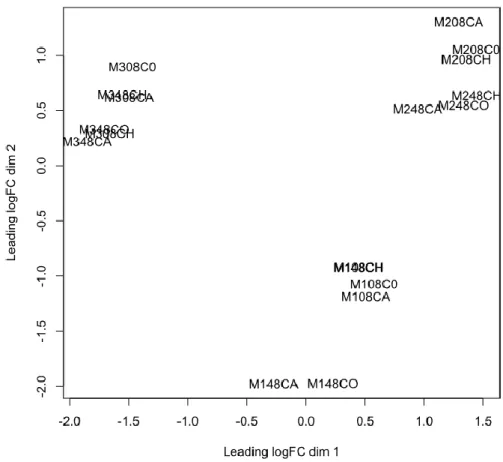
The MDS plot (Figure 3.4) shows that there was a fundamental flaw in the conception of this experiment. The experiment consisted of growing in culture the cells of 3 different animals from the same species and submit those cells to two types of stress while comparing it to a control. The plot shows three clusters, one cluster of all the samples marked as M3 which belong to the cells of mouse 3, another cluster containing the samples marked as M2 which belong to the cells of mouse 2 and another less defined cluster of samples of marked M1 which belong to cells of mouse 1. This can be assumed as a batch effect even though all steps of the experiment were done simultaneously there is clear difference because of where the cells came from.

(27)

17

Figure 3.4 MDS plot for the mouse samples

There were 4 comparisons that were biologically relevant in this experiment: comparing the control cells at 8 hours to the cells stressed with either camptothecin or chromium oxide and then the same thing for cells at 48 hours (Table 3.5).

Table 3.5 Number of differentially expressed genes in the mouse samples for each comparison

8h Con vs 8h Cam 8h Con vs 8h Chro 48h Con vs 48h Cam 48h Con vs 48h Chro Total genes 13440 13440 13440 13440 Up-regulated 0 0 0 0 Down-regulated 1 0 0 0

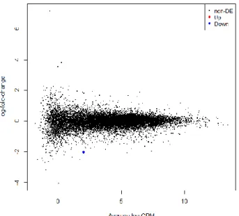
Despite the correction in the design matrix the distance shown on the MDS plot is simply too big. There are genes that are up-regulated and down-regulated but even though the correction to the design matrix worked because the values of the FDR decreased (Figure 3.6), there simply aren’t more genes in which the observed differential expression can be considered statistically significant.

(28)

18

Figure 3.5 Plot of up and down regulated genes in the 8h Con vs 8h Cam comparison. Only the colored dots are statistically relevant genes

The gene that is down-regulated in the mouse 8h Con vs 8h Cam comparison samples (the only blue dot in Figure 3.5) is Arhgef39, it has a log-fold-change of -2.0370377 (Figure 3.6) and its function is annotated as guanyl-nucleotide exchange factor activity.

Figure 3.6 Top 10 mouse genes with the lowest FDR in the 8h Con vs 8h Cam comparison. Above the top 10 genes before the adjustment to the design matrix. Below the top 10 genes after the adjustment.

(29)

19

Table 3.6 Normalization factors for the naked mole-rat samples

Sample Library Size Normalization Factor Sample N108CO 20933919 0.9357624 Sample N208CO 17258602 0.9870792 Sample N308CO 15112971 0.9911374 Sample N108CA 21354218 0.9900146 Sample N208CA 17269792 1.0504203 Sample N308CA 15726796 1.0266579 Sample N108CH 19914604 0.9488730 Sample N208CH 17586650 1.0113019 Sample N308CH 16395127 1.0369656 Sample N148CO 18606460 0.9146474 Sample N248CO 19946855 1.0414688 Sample N348CO 11912478 0.9868456 Sample N148CA 17317318 0.9781914 Sample N248CA 19537788 1.1065320 Sample N348CA 16504637 1.0355765 Sample N148CH 18160327 0.9467469 Sample N248CH 19565839 1.0413366 Sample N348CH 13777588 0.9897388

The MDS plot for the naked mole-rat data (Figure 3.7) shows the same type of clusters that the mouse MDS plot had in which the data clusters by animal. This was to be expected since the batch effect seems to be the origin of the cells and since these cells also came from three different animals it is normal that the naked mole-rat samples have the same type of problem as the mouse ones.

(30)

20

As with the mouse samples there aren’t many differentially expressed genes in the naked mole-rat samples due to the same problems the mouse samples had. The samples are simply too different and even if we try to account for that using the design matrix the picture doesn’t get much better (Table 3.7).

Table 3.7 Number of differentially expressed genes in the naked mole-rat samples for each comparison

8h Con vs 8h Cam 8h Con vs 8h Chro 48h Con vs 48h Cam 48h Con vs 48h Chro Total genes 14928 14928 14928 14928 Up-regulated 0 0 1 0 Down-regulated 0 0 0 0

The gene that is up-regulated in the naked mole-rat 48 hours camptothecin samples is Unc79. It has a log-fold-change of 1.2529478 (Figure 3.8) and is annotated as being involved in multicellular organism growth and behavioural response to ethanol. Unc79 has a mouse homolog (Keane et al., 2014), but in this experiment, Unc79 is one of the genes that is excluded from the analysis because it has a very low count in all the mouse samples. This gene is annotated as a behavioural response to ethanol and by being differentially expressed in this experiment, it may suggest that Unc79 could be an important player in naked mole-rat’s resistance against DNA-damaging compounds.

Figure 3.8 Top 10 naked mole-rat genes with the lowest FDR in the 48h Con vs 48h Cam comparison. Above the top 10 genes before the adjustment to the design matrix. Below the top 10 genes after the adjustment.

(31)

21

3.2 Experiment B

Table 3.8 Samples from Experiment B and the treatment they were subjected to

Sample Time Type of treatment Sample R148CO 48 hours Control Sample R248CO 48 hours Control Sample R348CO 48 hours Control Sample R196CO 96 hours Control Sample R296CO 96 hours Control Sample R396CO 96 hours Control

Sample R148BC 48 hours Gene Bc055324 silenced Sample R248BC 48 hours Gene Bc055324 silenced Sample R348BC 48 hours Gene Bc055324 silenced Sample R196BC 96 hours Gene Bc055324 silenced Sample R296BC 96 hours Gene Bc055324 silenced Sample R396BC 96 hours Gene Bc055324 silenced

3.2.1 Quality Control

The FastQC results were compiled with MultiQC, no further pre-processing was done because the files showed acceptable quality (Figure 3.9 - Figure 3.11). All files have very similar quality scores (Figure 3.9). All files show a mean quality Phred score over 30 across the length of the reads (Figure 3.9).

Figure 3.9 Mean quality scores across each base position in the read

Looking at the files by the quality scores per sequence (Figure 3.10), we can see that all the files have a high number of reads with Phred scores near 40, showing that there is quality in the sequencing.

(32)

22

Figure 3.10 Per sequence quality scores

The GC content graph is the most problematic from the FastQC reports. Some samples don’t seem very good (Figure 3.11) but all files present a distribution somewhat similar to a normal distribution. The green lines represent the samples that passed the quality control, the yellow lines indicate a warning and the red lines indicate the sample didn’t pass this quality control. Of the 24 files 8 failed this test, they were the reverse strands of samples R148BC, R196BC, R348CO, R196CO, R296CO, R396CO, R148BC, R348BC. The 7 files that got a warning were the forward strands of samples R296BC, R248BC, R348BC and the reverse strands of samples R296BC, R396BC, R248CO, R248BC. Meaning that samples R148BC, R348BC, R296BC had both the direct and reverse strand either with a warning or fail meaning they may be problematic samples. The two yellow lines that stand away from the back belong to the two files from sample R296BC. The three most problematic samples are all samples that were supposed to have the Bc055324 silenced, meaning that, that process may have contaminated those samples.

(33)

23

3.2.2 Mapping

Table 3.9 Results of mapping the samples to the human reference genome using STAR

Sample Number of input reads Percentage of uniquely mapped reads Sample R148CO 14615585 15.84% Sample R248CO 15123059 16.23% Sample R348CO 16604776 16.31% Sample R196CO 14655895 16.38% Sample R296CO 13118511 16.36% Sample R396CO 15053671 16.58% Sample R148BC 10409021 17.86% Sample R248BC 16867290 18.10% Sample R348BC 7515575 18.18% Sample R196BC 14773815 17.49% Sample R296BC 19891544 3.91% Sample R396BC 14778456 16.94%

The results from mapping the samples to the human reference genome using STAR indicate that there might be a problem with the samples (Table 3.8). The problems shown during the quality control steps couldn’t be responsible for this type of problem, though. While in Experiment A all samples had a percentage of uniquely mapped reads above 85%, there isn’t a single sample here higher than 19%. Sample R296BC is especially different suggesting something might have happened to that sample.

The first assumption made was maybe that since the sequencing for Experiment A was sent to sequencing at the same time as Experiment B there might I’ve been a mix up of samples. To evaluate this theory the samples were mapped simultaneously to the human, mouse and naked mole-rat using FastQ Screen (Figure 3.12, Figure 3.13, Figure 6.1 - Figure 6.22).

(34)

24

Figure 3.13 FastQ Screen results for file 2 of Sample R148CO

The results from FastQ Screen are very similar (Figure 3.12, Figure 3.13, Figure 6.1 - Figure 6.22) with only sample R296BC being a bit different (Figure 6.19, Figure 6.20) but consistent with the other results which suggest that the samples sequenced were all mouse samples. Since all the mouse samples from Experiment A mapped correctly to the mouse genome there doesn’t appear to be a mix up of samples between Experiment A and Experiment B. The Centre for Genomic Research at the University of Liverpool, where the sequencing was done, was contacted to enquire if there may have been a mix up and the wrong results delivered by them. The response was that, at the time of the sequencing of Experiment B, the only mouse samples they were sequencing were those from Experiment A, and since that hypothesis has already been excluded, that couldn’t be the origin of the problems. Before the sequencing was done, it was observed that Samples R148BC and R348BC had less material to be sequenced. In the results, Samples R148BC and R348BC are the samples with smallest number of reads which is consistent with the observation that they had the least amount to be sequenced.

All evidence points to the samples sent to sequencing being indeed mouse samples instead of human, indicating that the Experiment B had been executed with mouse cells instead of HeLa cells. How the mistake was made is unknown, the most likely hypothesis is there was a mislabelling of cells in the freezer. Since the mouse genome contains a homolog gene to Bc055324 (Zerbino et al., 2018) further analysis was carried on to see if any conclusions could be made even despite the mistake.

Table 3.10 Results of mapping the samples to the mouse reference genome using STAR

Sample Number of input reads Percentage of uniquely mapped reads Sample R148CO 14615585 84,03% Sample R248CO 15123059 85,96% Sample R348CO 16604776 85,47% Sample R196CO 14655895 86,32% Sample R296CO 13118511 81,91% Sample R396CO 15053671 84,22% Sample R148BC 10409021 80,27% Sample R248BC 16867290 85,19% Sample R348BC 7515575 78,05% Sample R196BC 14773815 85,08% Sample R296BC 19891544 86,40% Sample R396BC 14778456 84,91%

(35)

25

Mapping the samples to the mouse genome using STAR yielded satisfactory results consistent with the assumption that the samples were indeed mouse samples instead of human (Table 3.10).

Not all reads that were mapped using STAR map uniquely to exons of genes. Using ReadCounter we obtain read counts per gene that were uniquely mapped to exons of genes (Table 3.11). That information from all the samples is then compiled and processed using edgeR.

Table 3.11 Reads uniquely mapped to exons of genes using ReadCounter

Sample Number of reads uniquely mapping to exons of genes

Percentage of reads uniquely mapping to exons of genes Sample R148CO 10678411 86.95% Sample R248CO 10792708 83.03% Sample R348CO 12243843 86.27% Sample R196CO 10581730 83.64% Sample R296CO 9331954 86.85% Sample R396CO 10858397 85.64% Sample R148BC 7264609 86.95% Sample R248BC 12465888 86.75% Sample R348BC 5105414 87.03% Sample R196BC 11130728 88.55% Sample R296BC 2974825 17.31% Sample R396BC 11092144 88.39%

Another step where sample R296BC is problematic, after not mapping well to he human genome, it also didn’t map particularly well to the mouse genome, combining that the value of 30% of the sample mapping to an unknown sequence (Figure 6.19, Figure 6.20), it is almost certain that this sample had some sort of contamination. And if this experiment wasn’t already ruined it would be imperative to exclude this sample from the analysis.