Light field coding with field of view scalability and exemplar-based inter-layer prediction

Repositório ISCTE-IUL

Deposited in Repositório ISCTE-IUL:

Deposited version:

Peer-review status of attached file:

Citation for published item:

Conti, C., Soares, L. D. & Nunes, P. (2018). Light field coding with field of view scalability and exemplar-based inter-layer prediction. IEEE Transactions on Multimedia. 20 (11), 2905-2920

Further information on publisher's website:

10.1109/TMM.2018.2825882

Publisher's copyright statement:

This is the peer reviewed version of the following article: Conti, C., Soares, L. D. & Nunes, P. (2018). Light field coding with field of view scalability and exemplar-based inter-layer prediction. IEEE

Transactions on Multimedia. 20 (11), 2905-2920, which has been published in final form at https://dx.doi.org/10.1109/TMM.2018.2825882. This article may be used for non-commercial purposes in accordance with the Publisher's Terms and Conditions for self-archiving.

Use policy

Creative Commons CC BY 4.0

The full-text may be used and/or reproduced, and given to third parties in any format or medium, without prior permission or charge, for personal research or study, educational, or not-for-profit purposes provided that:

• a full bibliographic reference is made to the original source • a link is made to the metadata record in the Repository • the full-text is not changed in any way

The full-text must not be sold in any format or medium without the formal permission of the copyright holders. Serviços de Informação e Documentação, Instituto Universitário de Lisboa (ISCTE-IUL)

Av. das Forças Armadas, Edifício II, 1649-026 Lisboa Portugal Phone: +(351) 217 903 024 | e-mail: administrador.repositorio@iscte-iul.pt



Abstract— Light field imaging based on microlens arrays –

a.k.a. holoscopic, plenoptic, and integral imaging – has currently risen up as a feasible and prospective technology for future image and video applications. However, deploying actual light field applications will require identifying more powerful representations and coding solutions that support arising new manipulation and interaction functionalities. In this context, this paper proposes a novel scalable coding solution that supports a new type of scalability, referred to as Field of View scalability. The proposed scalable coding solution comprises a base layer compliant with the High Efficiency Video Coding (HEVC) standard, complemented by one or more enhancement layers that progressively allow richer versions of the same light field content in terms of content manipulation and interaction possibilities. Additionally, for achieving high compression performance in the enhancement layers, novel exemplar-based inter-layer coding tools are also proposed, namely: i) a direct prediction based on exemplar texture samples from lower layers, and ii) an inter-layer compensated prediction using a reference picture that is built relying on an exemplar-based algorithm for texture synthesis. Experimental results demonstrate the advantages of the proposed scalable coding solution to cater for users with different preferences/requirements in terms of interaction functionalities, while providing better rate-distortion performance (independently of the optical setup used for acquisition) compared to HEVC and other scalable light field coding solutions in the literature.

Index Terms— Light Field, Holoscopic, Plenoptic, Integral

Imaging, Field of View Scalability, Image Compression, HEVC

I. INTRODUCTION

HE recent advances in optical and sensor manufacturing allow having richer forms of visual data, where not only the spatial information about the three-dimensional (3D) scene is represented but also angular viewing direction – the so-called four-dimensional (4D) light field/radiance sampling [1]. In the context of Light Field (LF) imaging technologies, the approach based on a single-tier camera equipped with a Microlens Array (MLA) [2] (hereinafter referred simply to as LF camera) has become a promising approach, being applicable in many different areas of research, such as 3D television [3], richer photography capturing [4], [5], biometric recognition [6], and medical imaging [7].

Manuscript received March 24, 2018. This work was supported by FCT (Fundação para a Ciência e a Tecnologia, Portugal) under SFRH / BD / 79480 / 2011 grant and UID / EEA / 50008 / 2013 project.

C. Conti, L.D. Soares, and P. Nunes are with Instituto Universitário de Lisboa (ISCTE-IUL) and Instituto de Telecomunicações, Lisbon, Portugal (e-mail: {caroline.conti, lds, paulo.nunes}@lx.it.pt).

Recognizing the potential of this emerging technology, as well as the new challenges that need to be overcome for successfully introducing light field media applications into the consumer market, novel standardization initiatives are also emerging. Notably, the Joint Photographic Experts Group (JPEG) committee has launched the JPEG Pleno standardization initiative [8], and the Moving Picture Experts Group (MPEG) has recently started a new work item on coded representations for immersive media (MPEG-I) [9]. The challenge to provide a LF representation with convenient spatial resolution and viewing angles requires handling a huge amount of data and, thus, efficient coding becomes of utmost importance. Another key requirement when designing an efficient LF representation and coding solution is to facilitate future interactive LF media applications with the new manipulation functionalities supported by the LF content. The advantages of enabling interactive media applications has been previously studied in the literature for a large range of media modalities, such as: i) interactive streaming of high resolution images [10]; ii) interactive multiview video streaming [11], [12]; and iii) interactive streaming of light field images captured by high density camera-arrays [13]. In this context, although standardized LF representation and coding solutions are still in an early stage of development, various LF coding solutions have been already proposed in the literature.

A. Previous Work

LF coding solutions available in the literature can be categorized in the following three main approaches, depending on the data format and prediction schemes that are adopted. 1. LF raw data-based coding

This category corresponds to encoding and transmitting the (raw) LF image in its entirety. As a result of the used optical system, the LF image corresponds to a two-dimensional (2D) array of micro-images (MIs), and a significant cross-correlation exists between these MIs in a neighborhood [14]. To exploit this inherent MI cross-correlation, a non-local spatial prediction scheme is used, which is usually integrated (but not necessarily so) on a standard 2D image coding solution, such as the state-of-the-art High Efficiency Video Coding (HEVC). Following this approach, it has been shown, in [14]–[17], that efficient LF image coding can be achieved by using the concept of Self-Similarity (SS) compensated prediction. Similarly to motion estimation, a block-based matching algorithm is used to estimate the ‘best’ predictor block for the current block over the previously coded and reconstructed area of the current picture. This predictor block can be generated from a single candidate block [14], [15] or

Light Field Coding with Field of View Scalability

and Exemplar-Based Inter-Layer Prediction

Caroline Conti, Member IEEE, Luís Ducla Soares, Senior Member IEEE, and Paulo Nunes, Member

IEEE

from a combination of two different candidate blocks [16], [17]. Furthermore, an alternative prediction scheme based on locally linear embedding was proposed in [18], [19], where a set of nearest neighbor patches were linearly combined to predict the current block. More recently, in [20], a prediction scheme based on Gaussian Process Regression (GPR) was also proposed for LF image coding. In this case, the prediction was modeled from a set of nearest neighbor patches as a non-linear (Gaussian) process, and GPR was then used for estimating the predictor block.

However, although these coding schemes have shown to achieve significant compression gains when compared to state-of-the-art 2D image coding solutions [14]–[20], transmitting the entire LF data without a scalable bitstream may represent a serious problem since the end-user needs to wait until the entire LF data arrives before he/she can visualize and interact with the content.

2. Multiview- and PVS-based LF coding

Some other coding schemes proposed to extract the viewpoint images (VIs) from the LF content to be represented as multiview content [21]–[24], or as a Pseudo Video Sequence (PVS) [25]–[28]. In these coding approaches, each VI is constructed by simply extracting one pixel with the same relative position from each MI. The VI-based multiview content is then encoded using a 3D video coding solution, for instance, the Multiview Video Coding (MVC) [29] (in [21]– [23]) and the multiview extension of HEVC (MV-HEVC) [30] (in [24]). An advantage of using a standard 3D video coding solution is that scalability and backward compatibility are straightforwardly supported. Differently, the PVS of VIs is encoded using a 2D video coding standard, such as H.264/AVC [29] (in [25]), or HEVC [31] (in [26]–[28]). Although conceptually different (in terms of coding architecture), both multiview- and PVS-based coding approaches have the same basic purpose of providing an efficient prediction configuration for better exploiting the correlations between the views. For this, different scanning patterns for ordering the views, as well as different inter-view prediction structures are proposed in [21]–[27] to improve the coding efficiency.

However, although these approaches can provide scalability in the coded bitstream, it is possible to observe in the literature (e.g., in [15], [25], [27]) that their coding performance may vary significantly depending on the LF optical setup that is used for acquiring the LF content. As will be further discussed in Section II.B, there are basically two LF camera setups: i) unfocused (a.k.a. plenoptic camera 1.0); and ii) focused (a.k.a. plenoptic camera 2.0). For an LF image captured using the unfocused LF camera setup, each VI represents an orthographic projection of the captured scene that is all in focus [2]. On the other hand, for an LF image captured using a focused camera setup, a VI can be interpreted as a subsampled perspective of the captured scene (as in [32]) or as a low resolution rendered view that is all out of focus (as in [33]), which, consequently, presents aliasing artifacts. Furthermore, using an MLA with larger microlenses pitch leads to greater aliasing in the extracted VI [33]. Since these aliasing artifacts are difficult to predict and to compress, multiview- and PVS-based LF coding solutions usually present a significantly

worse coding performance for LF content captured using a focused LF camera setup (as shown in [15]).

It should be noticed that an alternative to the multiview representation based on these aliased VIs for focused LF cameras was proposed in [34], [35] using super-resolved rendered views. In this case, a scalable coding approach is used, which supports backward compatibility to legacy 2D and 3D multiview displays in the lower layer while the highest layer supports the entire LF content. However, with this coding architecture, the end-user still needs to receive the entire scalable bitstream to have a viewing experience with the novel interaction functionalities supported by the LF content. 3. Disparity-assisted LF coding

Other coding schemes proposed to represent the LF data by a subsampled set of MIs with their associated disparity information [36]–[38]. As firstly proposed in [39], the grid of MIs is subsampled to remove the redundancy between neighboring MIs and to achieve compression. Thus, only the remainder set of MIs and associated disparity are encoded and transmitted. At the decoder side, the LF data is reconstructed by simply applying a disparity shift (in [36], [38]) or by using a Depth Image Based Rendering (DIBR) algorithm modified to support the multiple MIs as input views (in [37]), and followed by an inpainting algorithm to fill in the missing areas. However, in real-world images, the disparity/depth information is estimated from the acquired LF raw data, which introduces some inaccuracies. Hence, the quality of the reconstructed MIs – and, consequently, the quality of rendered views – is severely affected by these inaccuracies at the encoder side. Additionally, due to occlusion problems and quantization errors when (lossy) encoding this disparity/depth maps, some synthesized MIs might present too many missing areas to be filled [37], thus introducing even further inaccuracies. Instead of uniformly selecting the MIs as in [38], the selection is performed adaptively in [36], [37], so as to obtain better view reconstruction.

However, a common characteristic of these approaches is that the quality of rendered views is negatively affected by the inaccuracies in the synthesis of the missing MIs, thus presenting a significant drop in the Peak Signal to Noise Ratio (PSNR) and Structural Similarity (SSIM) Index, mainly for natural content. In [38], the residue between the reconstructed LF image and the original LF image is also encoded and transmitted in an enhancement coding layer so as to provide better rendered views. Nevertheless, in this case [38], the end-user still needs to decode the entire scalable bitstream to visualize these rendered views with better quality.

B. Motivations and Contributions

Among the advantages of employing a LF imaging approach is the ability to open new degrees of freedom in terms of content production and manipulation, supporting manipulation functionalities not straightforwardly available in conventional imaging systems, namely: post-production refocusing, changing depth-of-field, and changing viewing perspective. This means, for instance, that the user can receive captured LF content and interactively adjust the plane of focus and depth-of-field of the rendered content. Moreover, as part of the creative process, the content creator can define how to

organize the LF content to be sent to multiple end-users who may be using different display technologies, as well as applications, that allow different levels of interaction. In this sense, an efficient scalable LF coding architecture is desirable to accommodate in a single compressed bitstream a variety of sub-bitstreams appropriate for users with different preferences/requirements and various application scenarios: from the user who wants to have a simple 2D version of the LF content without actively interacting with it; to the user who wants full immersive and interactive LF visualization.

Based on the abovementioned application scenarios, the contributions of this paper are:

 Field Of View (FOV) scalability – To support the richer and flexible interaction functionalities that arise in LF imaging applications, a new scalability concept, named FOV scalability, and a novel Field Of View Scalable Light Field Coding (FOVS-LFC) solution are proposed. Taking advantage of the 4D radiance distribution, the FOV scalability progressively supports richer forms of the same LF content by hierarchically organizing the angular information of the captured LF data. More specifically, the base layer contains a subset of the LF raw data with narrower FOV, which can be used to render a 2D version of the content with very limited rendering functionalities. Following the base layer, one or more enhancement layers are defined to represent the necessary information to obtain more immersive LF visualization with a wider FOV. Therefore, this new type of scalability creates bitstreams adaptable to different levels of user interaction, allowing increasing degrees of freedom in content manipulation at each higher layer. This means that, for instance, a user who wants to have a simple 2D visualization will only need to extract the base layer of the bitstream, thus reducing the necessary bitrate and the required computational power. On the other hand, a user who wants to creatively decide how to interact with the LF content can promptly start visualizing and flexibly manipulating the LF content, even over limited bandwidth connections, by extracting only the adequate bitstream subsets (which fit in the available bitrate). Additionally, this coding architecture enables easy support to quality scalability and Region Of Interest (ROI) coding [40].  Exemplar-based Inter-Layer (IL) coding tools – To improve the efficiency when coding an enhancement layer, two novel inter-layer prediction schemes are also proposed: i) a direct IL prediction, and ii) an IL compensated prediction. In the direct IL prediction, a set of samples from a previously coded layer is used as exemplar samples for estimating a good prediction block. Therefore, no further information about the used predictor block needs to be transmitted to the decoder side. The IL compensated prediction relies on an IL reference picture, which is constructed using samples from previously coded layers and a new exemplar-based [41] algorithm for texture synthesis.

In a nutshell, the proposed FOVS-LFC solution is able to overcome some of the limitations of previously proposed LF coding solutions by providing: i) a scalable bitstream that supports richer and flexible manipulation functionalities (such as refocusing, changing perspective and depth-of-field) and backward compatibility with the current state-of-the-art HEVC standard [31]; ii) support for quality scalability and

ROI coding; iii) high compression efficiency for LF content captured using different LF camera setups; as well as iv) high quality of rendered views in all hierarchical layers.

C. Paper Outline

The remainder of this paper is organized as follows. Section II briefly reviews the LF imaging principles that are important to understand the concepts discussed in this paper. Section III presents the concept of FOV scalability, while Section IV describes the FOVS-LFC solution architecture. Section V describes the exemplar-based inter-layer coding tools that are proposed for LF enhancement layer coding. Section VI presents the test conditions and experimental results; and, finally, Section VII concludes the paper.

II. LFIMAGING TECHNOLOGY

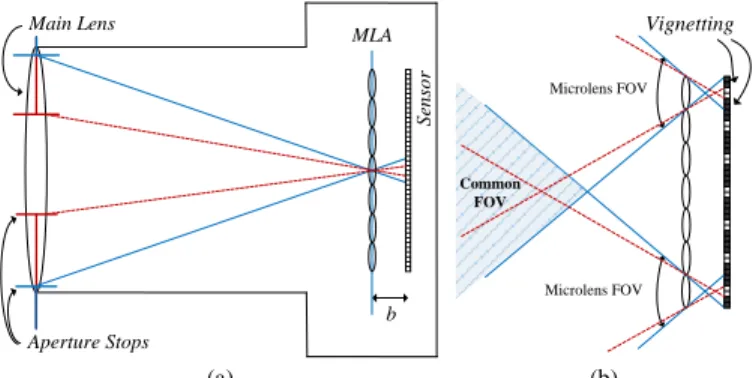
As illustrated in Fig. 1a, an LF camera basically comprises a main lens, and an MLA that lies at a distance 𝑏 of the image sensor. Therefore, different from a conventional 2D camera that captures an image by integrating the intensities of all rays (from all directions) impinging each sensor element (hereinafter referred to as pixel1_{) at position (x,y); in an LF} camera, each pixel collects the light of a single ray (or of a thin bundle of rays) from a given angular direction (θ,φ) that converges on a specific microlens at position (x,y) in the array. This means that it is possible to sample the 4D radiance and organize it in a conventional 2D image, known as the (raw) LF image.

To simplify the visualization of this 4D function (coordinates x, y, θ and φ), the flat Cartesian ray-space diagram [1], [42] shown in Fig. 2a is used in this paper, where only two dimensions – in this case, x and θ – are represented. A. LF Camera Setups

As discussed in [2], [33], different LF camera setups can be derived from the basic elements in Fig. 1a (i.e., a main lens, and an MLA at a distance 𝑏 of the image sensor), namely:  Unfocused LF camera – In this setup, the main lens is focused on the microlens plane while the microlenses are focused at infinity as illustrated in Fig. 2b (top) (the sensor is placed at the MLA focal length f, i.e., 𝑏 = 𝑓 in Fig. 1a). Moreover, since microlenses usually have a much smaller focal length than the main lens, it is reasonable to admit that the main lens is at the microlenses optical infinity. Consequently, the radiance coming from the captured scene is refracted through the main lens and then split by each microlens in the array. This can be seen in Fig. 2b (bottom), where the captured radiance is split into different columns corresponding to the bundle of rays sampled as an MI at the sensor. Afterwards, the light rays that hit a single microlens are separated into different angular directions to be projected onto the pixels in the image sensor underneath. Hence, each small rectangle in Fig. 2b, corresponds to the tiny bundle of rays (with width given by the microlens aperture, 𝑑) that is integrated into a single pixel of the MI. Examples of LF cameras using this setup are the Lytro LF cameras [5].

1 _{For the sake of simplicity, a pixel is here understood as a}

three-dimensional variable where each dimension contains the information of one color component: Red, Green, and Blue (RGB).

 Focused LF camera – As discussed in [2], [33], the unfocused LF camera (Fig. 2b) can be generalized to an alternative camera setup that is referred to as focused LF camera [33]. Examples of focused LF cameras are the Raytrix LF cameras [4]. In this setup, the main lens and the MLA are both focused in an image plane at a distance 𝑎 of the MLA plane, as illustrated in Fig. 2c (top). Thus, the main lens forms a relay system with each microlens, and the MLA works as a conventional camera array (with very low resolution and small baseline). As shown in [42], each MI will then capture what corresponds to a slanted stripe of the radiance (slope 𝑎−1_),

depicted by the ray-space diagram in Fig. 2c (bottom). Consequently, this configuration allows an effective increase in spatial resolution at the price of a decrease in angular resolution [2]. Comparing the ray-space diagram in Fig. 2b and c (bottom), it is possible to see that an MI captured using the focused LF camera setup contains more spatial information (at 𝑥 axis) than an MI captured using the unfocused LF camera setup (Fig. 2b). In a generalized LF camera, changing the distance 𝑏 will change the slope 𝑎−1 _in

Fig. 2c (bottom) and, consequently, the balance between providing larger angular or spatial resolution in the captured LF image [2]. A notable limit is when 𝑏 → 𝑓, 𝑎 → ∞, and this generalized setup corresponds to the unfocused LF camera. B. FOV in LF Cameras

The FOV of a lens (typically expressed by a measurement of area or angle) corresponds to the area of the scene over which objects can be reproduced by the lens. In a conventional 2D camera, the FOV is related to the lens focal length and the physical size of the sensor. In an LF camera, the microlens FOV is directly related to the aperture of the main lens. To illustrate this fact, Fig. 1a depicts the unfocused LF camera with two different aperture sizes (as shown by the blue and red aperture stops). As can be seen with the blue and the dashed red lines, all the rays coming from the focused subject will intersect at the MLA (at the image plane) and will then diverge until they reach the image sensor. Moreover, comparing the blue lines with the dashed red ones (in Fig. 1a), it is possible to see that the main lens aperture (or more

specifically, the F-number2 _{of the main lens) needs to be} matched to the F-number of the MLA to guarantee that MIs receive homogeneous illumination on their entire area, as seen in the blue line case (Fig. 1a). Otherwise, in the case of the dashed red line (Fig. 1a), pronounced vignetting (with the shape of the main lens aperture) will be visible in each MI, as illustrated in Fig. 1b.

Moreover, as depicted in Fig. 1b, the common area where the FOV of all microlenses overlaps can be seen as a measure of the amount of angular information in the captured LF content. Note that, if there is MI vignetting (see dashed red lines in Fig. 1b), the microlens FOV will be further restricted and, consequently, the angular information will be narrowed. This means that it is possible to control the amount of angular information that is available in the captured LF content by adjusting the main lens aperture. This fact has motivated the FOV scalability concept that is presented in the following.

III. THE FOVSCALABILITY CONCEPT

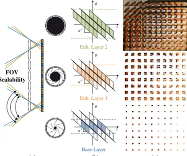
The basic idea of the proposed FOV scalability is to split the LF raw data into hierarchical subsets with partial angular information. Generally speaking, the FOV scalability can be thought of as a virtual increase in the main lens aperture (see Fig. 3a) from one scalable layer to the next higher layer, corresponding to a wider microlens FOV and virtual narrower vignetting inside each MI (along its border).

A. LF Data Organization for FOV Scalability

As was shown in Section II, each pixel underneath its corresponding microlens gathers light information from a given angular direction. Therefore, it is possible to split the overall angular information available in the captured LF image by properly selecting subsets of pixels from each MI. This concept is depicted in Fig. 3 for a hypothetical case in which three subsets of pixels are sampled from each MI. Therefore, the angular information is split into three hierarchical layers as seen in Fig. 3b (for the generalized focused LF camera setup). In each lower layer (from top to bottom in Fig. 3b), the 2 _{In optical terminology, the F-number corresponds to the ratio between the}

lens focal length and its aperture diameter.

(a) (b) (c)

Fig. 2 Parameterization of the 4D radiance in an LF camera: (a) A single light ray is described by the position it intersects the plane 𝑥 and its slope 𝜃. Each possible ray in the ray diagram (top) corresponds to a different point in the Cartesian ray-space diagram (bottom); (b) Sampling the radiance at the main lens image plane for the unfocused LF camera (when 𝑏 = 𝑓); and (c) Sampling the radiance at the image plane for the focused LF camera (when 𝑏 > 𝑓) ) x q x q Optical Axis Image Plane x q MI Pixel b= f x d d Image Plane x q Pixel MI b>f x d a a-1 d/a Image Plane (a) (b)

Fig. 1 LF camera: (a) Basic optical setup comprising a main lens, an MLA at a distance 𝑏 of the image sensor. Two aperture sizes are shown by the blue and dashed red lines; (b) The FOV can be used as a measure of overall angular information in the LF content. If the main lens and MLA F-numbers are not adjusted, the FOV is restricted and MI vignetting is observed

b S en so r MLA Main Lens Aperture Stops Vignetting Microlens FOV Common FOV Microlens FOV

microlenses FOV will be further restricted (see Fig. 3a) and, consequently, the angular information of the system will be narrowed.

The angular information is chosen to grow from the central to the border pixels in each MI due to two essential reasons: i) the central angular direction is usually the perspective the shooter will point towards when capturing the LF image; and ii) pixels at the MI border are usually more affected by optical and geometric distortions than the central pixels. As an illustrative example, Fig. 3c shows the selection of the three subsets of pixels with different angular information from each MI to build a FOV scalable data format. For the base layer in Fig. 3c (bottom), only a set with central angular information is gathered. For the enhancement layers 1 and 2 in Fig. 3c (respectively, middle and top), the samples progressively contain wider angular information (from the center to the borders).

Due to the nature of the LF imaging technology, where angular (θ,φ) and spatial (x,y) information is spatially arranged in a 2D image (i.e., the LF image), the increased angular information in each higher FOV scalable layer implies also an increase in the mega-ray3 _{resolution of the LF content} in the layer. This means that resolution scalability is inherently associated to the FOV scalability (see Fig. 3c).

It is also important to notice that the FOV scalable LF data format is always restricted by the optical setup used when acquiring the original LF content. For instance, the total amount of angular information that is available to be subsampled in each MI is controlled by:

3 _{Mega-ray is a measure of light field data capture that corresponds to the}

number of rays that are captured by the image sensor. This is numerically given by the resolution of the LF camera image sensor.

 Real aperture size – As seen in Section II.B, the (real) main lens aperture used in the LF content acquisition controls the amount of light angular information that is admitted through the LF camera optical system and that is sampled by the MIs.

 Distance 𝑏 in the generalized (focused) LF camera – As discussed in Section II.A, the distance 𝑏 (Fig. 1a) controls the balance between angular and spatial resolution in the captured LF image. Then, the closer 𝑏 is to the MLA focal length, 𝑓, the wider angular information is sampled by the MIs (Fig. 2). B. Application of the FOV Scalability for Flexible Interaction The great advantage of the proposed FOV scalable data format is the increased flexibility it gives to the authoring process. This means that the content creator is able to select the number of hierarchical layers and the size of the subset of pixels to be sampled for each layer as a part of the creative process.

With this format, it is possible to define new levels of scalability, for instance, in terms of the following rendering capabilities:

 Changing perspective – It is straightforward to see that narrowing the FOV of each MI will limit the angular information in lower scalable layers and, consequently, the number of different viewpoint perspectives that are possible to render. Therefore, the higher the layer is, the greater the number of available viewpoints is for the user’s interaction.

 Changing focus (refocusing) – Refocusing can be seen as

virtually translating the image plane of the LF camera to another plane in front or behind it. Briefly, narrowing the FOV of the MI in each scalable layer will result in fewer depth planes that are available for refocusing. Hence, the higher the layer is, the richer the refocusing range is for the user’s interaction.

 Varying depth-of-field – Increasing or decreasing the depth-of-field in LF images simply means to define larger or smaller (discrete) numbers of depth planes to be in focus simultaneously. Similarly to refocusing, limiting the MI angular information in each scalable layer will also limit the number of planes that are available to be in focus. Therefore, the higher the layer is, the deeper is the depth-of-field that can be selected during the user’s interaction.

Therefore, the author can decide which perspective(s) and depth plane(s) need to be in focus when presenting the content in each of the hierarchical layers. Depending on his/her decision, narrower or wider angular information needs to be gathered for these layers.

C. LF Data Organization for ROI Coding

Another advantage of the proposed FOV scalable data format is the ability to enable easy integration of ROI coding [40], [43]. ROI coding can be an important functionally, especially in limited network channels [43], in applications scenarios where some portions of the visualized content are of higher importance than others. In the proposed FOV scalable data organization, this functionality would allow further flexibility in the bitstream for supporting the new interactive manipulations capabilities in the LF visualization.

For instance, for an LF image with very large resolution, the size of the compressed bitstream may be still considerably big

(a) (b) (c)

Fig. 3 The concept of FOV Scalability for a hypothetical three-layer approach: (a) Ray tracing diagram showing that three hierarchical layers of FOV Scalability can be sampled by properly selecting three subsets of pixels (with different colors) from each MI, corresponding to a virtual increase in the main lens aperture; (b) Corresponding ray-space diagram showing the angular information in each hierarchical layer; and (c) Illustrative example for gathering the three subsampled set of pixels from each MI. From the base layer (bottom) to the last enhancement layer (top), the FOV is wider and, consequently, the LF content resolution progressively grows as well

FOV Scalability Enh. Layer 2 x q a-1 Enh. Layer 1 x q a-1 Base Layer x q a-1

in some LF enhancement layers to be streamed efficiently. Thus, a solution would be to send in these layers only a portion of the image which is of the most interest (i.e., the ROI) with wider FOV. Therefore, the end-user receives a coarse version of the LF content in the base layer and, if the network conditions permit, he/she has the option of interactively refining a portion or portions of the coarse received LF content with the new manipulation functionalities (such as refocusing, changing perspective and depth-of-field) by decoding further enhancement layers.

Fig. 4 illustrates this concept for a hypothetical case in which three hierarchical layers are defined. In the base layer (bottom), a coarse version of the LF content is gathered with very restricted FOV. Following this, there is a great variety of options for defining the ROI enhancement layers. Two of these possibilities are depicted in Fig. 4a and b. In Fig. 4a, the highest ROI enhancement layer (top) considers the same ROI as the previous layer, but with wider FOV. Differently, in Fig. 4b, the highest ROI enhancement layer considers the same FOV as the previous layer but increases the ROI size. In both cases, a similar amount of texture information is gathered in the highest layer.

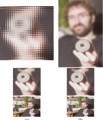
Additionally, Fig. 5 illustrates examples of refinements, in terms of FOV manipulation functionalities, which can be allowed by using the ROI enhancement layers defined in Fig. 4a. Fig. 5a shows a central view rendered from the coarse version of the LF content in the base layer. In this case, the amount of LF information that is coded and transmitted is

about 6 times less compared to the complete three-layered scalable bitstream in Fig. 4a. However, it can be seen that this significant reduction in terms of bits comes at the expense of limited FOV manipulation functionalities. For instance, it is not possible for an end-user to adjust the focus at the object in the man’s hand, since it is outside the refocusing range allowed in the base layer (Fig. 4a). Differently, Fig. 5b depicts the refinement in the plane of focus that becomes available when decoding the ROI enhancement layer 2.

Moreover, Fig. 5c illustrates a possible refinement in the rendered view perspective that becomes available in the ROI enhancement layer 2. In this case, the perspective is slightly changed inside the ROI (to the left) while fixing the non-ROI

(a) (b)

Fig. 4 Illustrative examples for gathering three hierarchical layers from the base layer (bottom) to the last enhancement layer (top) to enable the ROI functionality. The amount of information gathered in each layer is depicted with proportional sizes: (a) The last ROI enhancement layer (top) considers the same ROI as the previous layer, but with wider FOV; (b) The last ROI enhancement layer (bottom) considers the same FOV as the previous layer but with a larger ROI.

(a)

(b)

(c)

Fig. 5 Examples of refinements in terms of refocus and perspective manipulation functionalities allowed by using the ROI enhancement layers in Fig. 4a: (a) The central view rendered from the coarse version of the LF content available in the base layer; (b) The refinement in the plane of focus when overlaying the ROI enhancement layer 2, for focusing at the object on the man’s hand; and (c) Changing the perspective (to the left) inside the ROI while fixing the non-ROI area in the central view.

area in the central view. It should be noticed that some blending inconsistencies may appear, in this case, where the ROI and non-ROI join, (e.g., in the man’s beard and knee in Fig. 5c). A possible solution to this is to use an arbitrarily shaped ROI instead of a rectangular one. This solution will be considered in the future work.

IV. PROPOSED FOVS-LFCARCHITECTURE

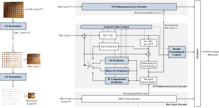
The coding architecture adopted in the proposed FOVS-LFC solution is built upon a predictive and multi-layered approach, as depicted in Fig. 6.

A. Coding Flow

The coding information flow in the proposed FOVS-LFC architecture is presented in the following:

 LF decimation – As illustrated in Fig. 6a, the LF data is firstly decimated into several layers, where higher layers contain LF content with wider FOV. In this process, the content creator will select the number of hierarchical layers and the size of the subset of pixels to be sampled for each layer. The decision of having narrower or wider angular information in each hierarchical layer may be made, for example, targeting a set of particular application scenarios. The base layer contains a sub-sampled portion of the LF data, which can be used to render a 2D version of the content with limited interaction capabilities (narrow FOV, limited in focus planes, and shallow depth-of-field). As shown in Fig. 6b, this base layer is coded with a conventional HEVC intra encoder to provide backward compatibility with a state-of-the-art coding solution, and the reconstructed picture is used for coding the higher layers. Following the base layer, one or more enhancement layers (enhancement layers 1 to N in Fig. 6a) are defined to represent the necessary information to obtain more immersive LF visualization. Each higher enhancement layer picture contains progressively richer angular information, thus increasing the LF data manipulation

flexibility. Finally, the last enhancement layer represents the additional information to support full LF visualization with maximum manipulation capabilities. Each enhancement layer is encoded with the proposed LF enhancement layer codec seen in Fig. 6b, which is based on the HEVC architecture and uses the following new and modified modules:

 Direct IL prediction – To improve the RD performance when coding an LF enhancement layer, a new direct IL prediction is proposed, as shown in Fig. 6b. This direct IL prediction aims at exploiting the redundancy between adjacent layers to implicitly derive an IL predictor block for encoding the current block in an LF enhancement layer picture. As a result, the decoder can simply use the same process for inferring the predictor block. To avoid further signaling, only an index is transmitted together with the coded residual information, which is used to distinguish the direct IL prediction from the conventional HEVC merge mode [31]. The process to derive the direct IL predictor is presented in Section V.A.

 IL compensated prediction – A new IL compensated prediction can also be used to further improve the LF enhancement layer coding efficiency by removing redundancy between adjacent layers. For this, an enhanced IL reference picture is constructed and used as a new reference picture when encoding the current LF enhancement layer picture. To construct this enhanced IL reference picture, an exemplar-based texture synthesis algorithm is used, which is presented in Section V.B. If this IL prediction mode is used, the residual information and an IL vector are coded and transmitted to the decoder side.

 SS prediction – Since the proposed FOV scalable data organization still presents high redundancy between adjacent MIs (or decimated MI texture samples), the SS prediction (see Section I.A.1), previously proposed by the authors [15], can also be used as an alternative prediction to exploit this existing MI redundancy and to improve coding efficiency within each

(a) (b)

Fig. 6 The FOVS-LFC architecture (novel and modified blocks are highlighted in blue): (a) The LF decimation process to generate content for each hierarchical layer; (b) Proposed coding architecture in which one or more enhancement layers (from 1 to N-1) are coded with the proposed LF enhancement encoder

LF Decimation .. . Base Layer (Layer 0) Enh. Layer 1 LF Decimation Enh. Layer N-1 Enh. Layer N Decoded Picture Buffer

-HEVC Intra Encoder

FOV Scalable Bitstream Deblocking & SAO Filtering Inv. SQ / Inv. DCT Header Formatting & CABAC Intra Prediction

Base Layer Encoder

Direct IL Prediction

Reconstructed Enh. Layer 1

LF Enhancement Layer Encoder

.. . Enh. Layer N Enh. Layer 1 Base Layer (Layer 0)

LF Enhancement Layer Encoder

Reconstructed Base Layer Reconstructed Enh.Layer N-1

General Coder Control

DCT/ SQ SS Prediction M u lt ip le x IL Compensated Prediction

LF enhancement layer. As a result, the residual information and SS vector(s) are coded and sent to the decoder.

 General coding control –The decision among using conventional HEVC intra prediction, SS, direct IL and IL compensated prediction is made in a Rate-Distortion (RD) optimization manner [44].

Header formatting & Context-Adaptive Binary Arithmetic Coding (CABAC) – Additional syntax elements are carried

through the high-level syntax bitstream to support FOV scalability. These are acquisition information (e.g., MI resolution and LF decimation information) and dependency information (for signaling the use of SS and IL prediction). Residual and prediction signaling are coded using CABAC.

B. Quality Scalability and ROI Coding Support

In addition to the FOV scalability, other functionalities are straightforwardly supported by the proposed FOVS-LFC solution, notably:

 Quality Scalability – Quality scalability can be achieved by quantizing the residual texture data in an LF enhancement layer with a smaller Quantization Parameter (QP) size relative to that used in the previous hierarchical layer. The QP values to be used in each layer can be adaptively adjusted to achieve the best tradeoff between quality and bitrate consumption.  ROI Coding – In this case, the encoder can send, in different FOV enhancement layers, the information of the ROI with richer manipulation capabilities and better visual quality, at the expense of limited manipulation capabilities and potential lower visual quality in the background. For this, an adaptive quantization approach can also be used to proper assign reasonable bit allocation among different scalable layers.

V. EXEMPLAR-BASED ILCODING TOOLS

To achieve a high coding efficiency, the proposed FOVS-LFC solution relies on two exemplar-based IL coding tools detailed in this section: i) direct IL prediction, and ii) IL compensated prediction.

A. Direct IL Prediction

Similarly to template matching [45], the proposed direct IL prediction uses an implicit approach to avoid transmitting any information about the used predictor block. Hence, the decoder can simply use the same process for inferring the predictor block to be used for reconstructing the current block (using the decoded residual information).

The process to derive the IL predictor block can be divided in the following two steps.

1. Exemplar Block Derivation

In this first step, an exemplar-block is derived using the coded and reconstructed samples from a previous FOV scalable layer (referred to as the reference layer). This exemplar-block will then be used for implicitly finding a prediction to the current block, 𝐼(𝐱), at position 𝐱 = (𝑥, 𝑦) in the LF enhancement layer picture being coded (referred to as current layer).

Since a lower layer has narrower FOV and, consequently, a

lower number of texture samples, it is firstly necessary to re-organize the texture information to align the MI samples from the reference layer according to the MI samples in the current layer. As a result, the reference layer is then represented as a picture with the same spatial resolution of the current layer picture and comprising a sparse set of known MI samples, as illustrated by the gray blocks in Fig. 7. This sparse picture is hereinafter referred to as sparse IL reference picture.

As the output of this step, an exemplar block, 𝑃(𝐱), with the same size and co-located position to the current block, 𝐼(𝐱), is derived from the sparse IL reference picture (Fig. 7).

2. Direct IL Prediction Estimation

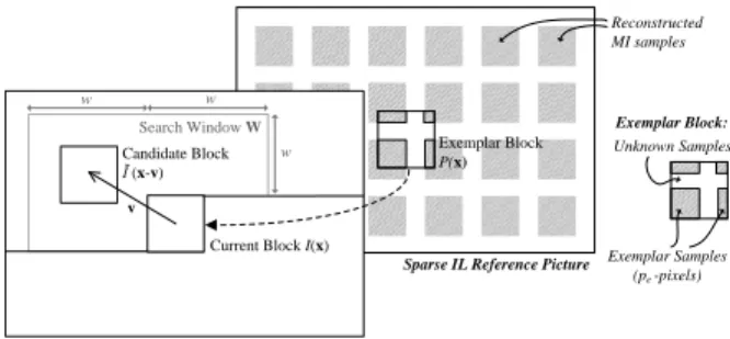
In this step, the exemplar block, 𝑃(𝐱), that was derived in the previous step is used as a template (similarly to template matching [45]) for estimating the ‘best’ predictor block to the current block, 𝐼(𝐱). For this, a matching algorithm is used to find the candidate block that ‘best’ agrees with 𝑃(𝐱) in the previously coded and reconstructed area of the current layer picture (Fig. 7). However, the ‘best’ candidate block is chosen by matching only the known samples of 𝑃(𝐱) (referred to as exemplar samples), since these are the only samples available at the decoding time.

Therefore, let 𝑃(𝐱) be a column vector containing the 𝑝-pixel samples of the exemplar block, where only the 𝑝𝑒-pixel

exemplar samples (Fig. 7) are known at decoding time. Also, let 𝐼̃(𝐱 − 𝐯) be a column vector containing the 𝑝-pixel previously coded and reconstructed samples of a candidate predictor block in the current layer picture (Fig. 7). This candidate predictor block is displaced from 𝐼(𝐱) by the vector 𝐯 (Fig. 7). Since 𝑃 contains (𝑝 − 𝑝𝑒) unknown samples, it can

be modeled as P =A Ĩ, where 𝐀 is a binary mask in which only the corresponding known 𝑝𝑒 sample positions are non-zero.

Thus, 𝐀 can be represented as a 𝑝 × 𝑝 binary diagonal matrix whose (𝑝 − 𝑝𝑒) unknown diagonal samples are set to zero.

Finally, since the mask 𝐀 is known a priori, the ‘best’ candidate predictor block can be simply found by solving the matching algorithm in (1).

min

𝐯,𝐼̃(𝐱−𝐯) ⊂𝐖 ‖𝑃(𝐱) − 𝑨 𝐼̃(𝐱 − 𝐯)‖1 (1)

To keep the complexity low, the predictor block is searched inside a limited search window, 𝐖, as depicted in Fig. 7 (i.e., 𝐼̃(𝐱 − 𝐯) ⊂ 𝐖), and the ℓ1-norm (or the sum of absolute

differences), ‖ ‖₁, is used as the matching criterion in (1).

Fig. 7 Exemplar-based direct IL prediction, where an implicit predictor block for the current block is estimated by solving (1). In this process, the candidate block (within the search window W in the current layer picture) that ‘best’ agrees with the exemplar block is chosen as the predictor block.

Sparse IL Reference Picture

Unknown Samples

Exemplar Samples (pe -pixels)

Current Layer Picture

Search Window W

Current Block I(x)

Exemplar Block P(x) Reconstructed MI samples Exemplar Block: Candidate Block Ĩ (x-v) v w w w

B. IL Compensated Prediction

To further improve the LF enhancement layer coding efficiency, an IL compensated prediction is also proposed, which relies on an enhanced IL reference picture. This section describes the process for building the enhanced IL reference. 1. Input Information

The input information for this process is the coded and reconstructed samples from a reference layer picture that are properly aligned to the MI samples in the current layer picture. As seen in Section V.A.1, this re-arrangement results in the sparse IL reference picture (Fig. 7) that comprises a sparse set of known MI samples, as depicted in Fig. 8.

This sparse IL reference picture is used as the basis for building the enhanced IL reference picture. In this process, an exemplar-based texture synthesis algorithm is used to find a good estimation to fill in the unknown data in the sparse IL reference picture. This is clearly an ill-posed problem; however, it is still possible to obtain a realistic approximate solution by imposing additional constraints coming from the physics of the problem. This is done here by using the prior knowledge that neighboring MI samples present significant cross-correlation, and for this reason, it is likely to find the unknown region of a particular MI in an area of neighboring MIs. This problem is formalized as follows.

2. Problem Formulation

Firstly, the unknown pixels in the sparse IL reference picture are set to zero. Moreover, this sparse IL reference picture is divided into 𝑛-pixel non-overlapping patches, 𝜙𝑠, to

apply the texture synthesis algorithm (Fig. 8). Each patch is then given by 𝑛𝑠 known samples – referred to as the support

samples – and (𝑛 − 𝑛𝑠) unknown samples to be synthesized

(Fig. 8). Hence, each patch can be represented as the product of a texture column vector, 𝜙𝑠, and a binary mask, 𝐒, in which

all but (𝑛 − 𝑛𝑠) samples have value equal to one. The binary

mask 𝐒 is given by an 𝑛 × 𝑛 binary diagonal matrix with the respective (𝑛 − 𝑛𝑠) unknown diagonal samples set to zero.

Accordingly, the goal of the texture synthesis algorithm is to find an 𝑛-pixel exemplar patch 𝜙𝑒𝑏𝑒𝑠𝑡(𝐱 − 𝛚) in the sparse

IL reference picture – at position (𝐱 − 𝛚) – that ‘best’ agrees with the support samples of the patch 𝜙𝑠(𝐱) at position 𝐱 =

(𝑥, 𝑦). To solve this, it can be assumed, without loss of generality, that the exemplar patch can be found in a neighborhood, 𝛀, of 𝐱 (i.e., 𝜙𝑒𝑏𝑒𝑠𝑡(𝐱 − 𝛚) ⊂ 𝛀) comprising 𝐾

neighbor MIs (i.e., 𝛀 = {𝑀𝑘}𝑘=1…𝐾 where 𝑀𝑘 denotes an MI)

as shown in Fig. 8. Additionally, it is assumed that a candidate exemplar patch 𝜙𝑒 comprises only 𝑛𝑒 known pixels.

Consequently, it can also be represented as the product of a texture column vector, 𝜙𝑒, and an 𝑛 × 𝑛 binary diagonal

matrix, 𝐄, with (𝑛 − 𝑛𝑒) diagonal samples set to zero.

Therefore, the best exemplar patch, 𝜙𝑒𝑏𝑒𝑠𝑡, can then be

found by solving the optimization problem in (2), min

𝜙_𝑒(𝐱−𝛚)⊂ 𝛀,𝐀 ‖𝐁 ⋅ (𝜙𝑠(𝐱) − 𝜙𝑒(𝐱 − 𝛚))‖1

+ 𝜆 × ‖𝑑𝑖𝑎𝑔(𝐈𝑛− 𝐁)‖0

(2) where 𝐁 corresponds to a binary diagonal matrix that

represents the samples from 𝜙𝑠 and 𝜙𝑒 that overlap (i.e., 𝐁 =

𝐒 ⋅ 𝐄); 𝐈𝑛 corresponds to an 𝑛 × 𝑛 identity matrix; 𝑑𝑖𝑎𝑔( )

denotes a vector of the diagonal elements of a matrix; and ‖ ‖₁ e ‖ ‖0 denote ℓ1 and ℓ0 norms, respectively.

The problem in (2) comprises a data-fitting term and a sparseness prior function, respectively. The former term tries to find the best match within the region where 𝜙𝑠 and 𝜙𝑒

overlap, while the latter term penalizes candidate patches whose 𝑛𝑒-pixel region is too small. In addition to this, since

the border of the MIs typically exhibits high intensity variations (mainly due to the vignetting), a further constraint is imposed to the problem formulated in (2) to guarantee that these high frequency samples from the borders of an MI sample, 𝑀k⊂ 𝛀, do not affect negatively the synthesized

patterns, which is to solve the problem in (2), subjected to: (𝜙𝑒(𝐱 − 𝛚) ∈ 𝑀𝑘) ∩ (𝜙𝑒(𝐱 + 𝛚) ∉ 𝑀𝑚≠𝑘) = { }.

In the experimental results presented Section VI, the λ value (2) is selected empirically, and the patch size is selected to be a quarter of the size of an MI sample in the current layer.

The presented exemplar-based solution is chosen due to its simplicity and effectiveness for tackling the proposed problem. However, better solutions might still be formulated, for instance, by adding an edge-preserving regularizer in (2), or by using superpixel-based inpainting [46]. Moreover, although the angular information is limited in each subsampled MI in a lower layer, it is still possible to derive disparity or ray-space information to reconstruct the discarded 4D radiance samples at the receiver side. These solutions are left for future work.

3. Texture synthesis

Once the best patch 𝜙𝑒𝑏𝑒𝑠𝑡 is obtained by solving (2), the

synthesized region is derived by simply copying the samples of the region defined by 𝐄 ∖ 𝐁. This optimization process is iteratively repeated until all unknown samples are filled in or until the number of unknown samples stabilizes (i.e., the number of unknown samples remains the same between two iterations). Thus, at each iteration, the values of 𝜙𝑒 and 𝐁 are

updated from the values found in the previous iteration. As an illustrative example, Fig. 9 shows a portion of the constructed enhanced IL reference picture for the LF enhancement layer 2 illustrated in Fig. 3c (top).

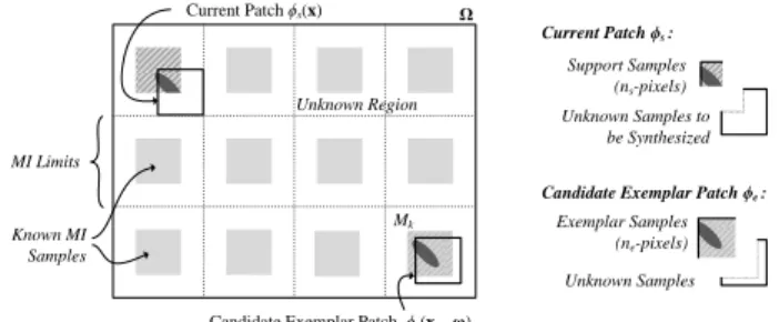
Fig. 8 Exemplar-based texture synthesis algorithm for building an enhanced IL reference picture. For each patch 𝜙𝑠 in the sparse IL reference picture, the

‘best’ candidate exemplar patch, 𝜙𝑒𝑏𝑒𝑠𝑡, is derived by solving the optimization

problem in (2).

Unknown Region

Known MI Samples

Candidate Exemplar Patch ϕe(x – ω)

Current Patch ϕs(x) Unknown Samples to be Synthesized Support Samples (ns-pixels) MI Limits Ω Current Patch ϕs :

Candidate Exemplar Patch ϕe :

Exemplar Samples (ne-pixels)

Unknown Samples Mk

VI. PERFORMANCE ASSESSMENT

This section assesses the performance of the proposed FOVS-LFC solution. For this purpose, the test conditions are firstly introduced and, then, the obtained experimental results are presented and discussed.

A. Test Conditions

The performance assessment considered the following test conditions:

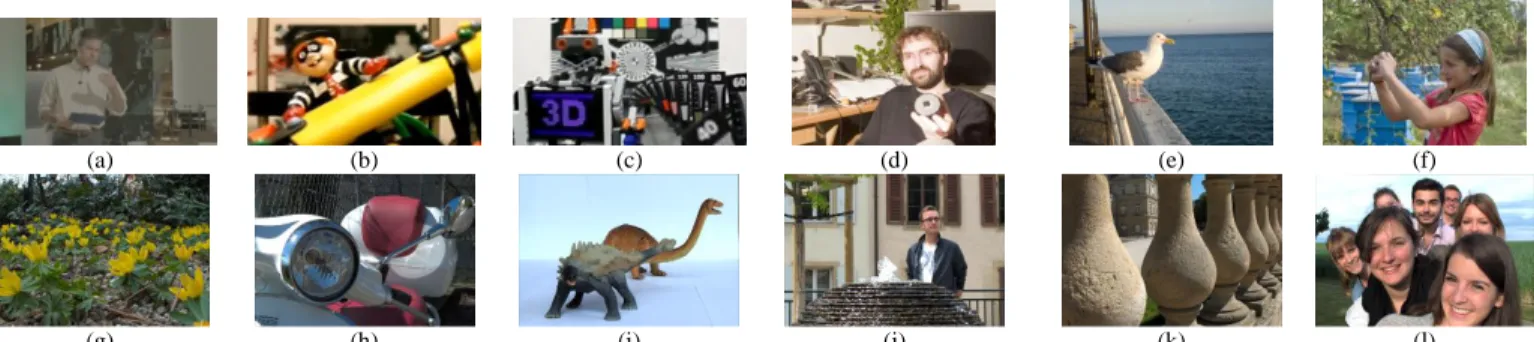
 LF Test Images – Twelve LF test images captured using different optical acquisition setups and with different scene characteristics are used, as shown in Fig. 10 and Table I. Before being coding, the raw LF images were pre-processed in order to: i) align and center the microlens grid to the pixels grid; ii) discard incomplete MIs (at the border of the LF image) iii) transform from hexagonal to rectangular microlens grid (only if necessary, see Table I); and iv) correcting color and gamma. As suggested in [47], only after this pre-process the LF image was convert to Y’CbCr 4:2:0 color format (8 bits) to avoid decreasing the visual quality after coding [47]. For LF test images whose calibration information was available (i.e., Fig. 10g to l), the Matlab LF Toolbox [48] was used for the pre-processing. It is worth noting that transforming from hexagonal to rectangular grid with the Matlab LF Toolbox results in an LF image with multiple black pixels at the MIs border. These black pixels were also discarded when pre-processing the LF test images. For the remaining LF test images (i.e., for the LF images in Fig. 10a to Fig. 10f, whose calibration information was not available), a DCT-based interpolation filter [49] was used for aligning and centering the microlens grid.

 LF Decimation – To generate the content for each hierarchical layer, l, in the FOVS-LFC solution, a central texture sample block with size (2l+2×2l+2) is selected from each MI in the LF image to support FOV scalability. These

squared texture sample blocks with a power of two size were here chosen to better fit into the CTU and PU partition patterns of HEVC [31]. However, the proposed scalable codec can be generalized for any texture sample block size and aspect ratio. The number of hierarchical layers varies for each LF test image and is given by ⌈1 2⁄ log2𝑀⌉ for a squared MI

with 𝑀 × 𝑀 pixels size (see Table I). Finally, the highest layer contains the entire LF image, whose resolution is shown in Table I. No ROI coding is considered in order to analyze the worst-case scenario in terms of the amount of texture information that is coded in each hierarchical layer.

 Codec Software Implementation – The MV-HEVC reference software version 12.0 [30] is used as the base software for implementing the proposed FOVS-LFC codec.  Coding Configuration – Each LF test image is encoded using four different Quantization Parameter (QP) values: 22, 27, 32, and 37, according to the HEVC common test conditions defined in [50]. The same QP value is used for coding all hierarchical layers in order to analyze the worst-case scenario in terms of bitrate allocation. For both exemplar-based IL prediction and for the SS prediction, a search window with w= 128 (see Fig. 7) is adopted.

 RD Evaluation – For evaluating the overall RD performance of the proposed FOVS-LFC codec, two different objective quality metrics are considered, which are referred to as: i) Overall PSNR_Y; and ii) Rendering-dependent PSNR_Y. The overall PSNR_Y is calculated by taking the average luma Mean Squared Error (MSE̅̅̅̅̅̅) over the pictures in each hierarchical layer, and, then, converting it to the PSNR. Differently, the rendering-dependent PSNR_Y is measured in terms of the average luma PSNR calculated from a set of views rendered from the reconstructed LF content, similarly to the metrics proposed in [8]. To have a representative number of rendered views, a set of 11×11 views was rendered from uniformly distributed directional positions. For rendering the views from LF images captured using a focused LF camera setup, the algorithm proposed in [33] and referred to as Basic Rendering algorithm was used. In this case, the plane of focus was chosen to represent the case where the main object of the scene is in focus. For LF images captured using the unfocused LF camera setup, 11×11 VIs were extracted. The rate is calculated as the total number of bits needed for encoding all scalable layers divided by the number of pixels in the LF image given in Table I (bpp).

In addition, the performance of the proposed FOVS-LFC solution is compared to the following solutions:

(a) (b) (c) (d) (e) (f)

(g) (h) (i) (j) (k) (l)

Fig. 10 Example of a central view rendered from each light field test image: (a) Demichelis Spark [53], (b) Plane and Toy [53]; (c) Robot 3D [53]; (d) Fredo [54], (e) Seagull [54], (f) Laura [54], (g) Flowers [55], (h) Vespa [55], (i) Ankylosaurus_&_Diplodocus_1 [55], (j) Fountain_&_Vincent_2 [55], (k) Stone_Pillars_Outside [55], and (l) Friends_1 [55]

(a) (b)

Fig. 9 A portion of the enhanced IL reference picture built for the enhancement layer 2 in Fig. 3c: (a) the sparse IL reference picture; (b) the enhanced IL reference picture built by solving (2); and, (c) the difference to the original LF enhancement picture

 HEVC (Single Layer) – In this case, the entire LF raw data is encoded into a single layer with HEVC using the Main Still Picture profile [31].Since the proposed FOVS-LFC codec provides an HEVC-compliant base layer, this solution is used as the benchmark for non-scalable LF coding to compare the bit savings with the proposed scalable LF coding solution. Thus, it would correspond to the ideal RD performance if scalability was supported without any rate penalty.

 FOVS-LFC (Simulcast) – This solution corresponds to the benchmark for the simulcast case, where all pictures from each hierarchical layer are coded independently with HEVC intra coding. For this, the MV-HEVC reference software version 12.0 is used with “All Intra, Main” configuration [50].  FOVS-LFC (SS Simulcast) – In this case, each picture from each hierarchical layer is coded with the FOVS-LFC codec but only enabling the SS prediction and conventional HEVC intra prediction. Hence, not only local spatial prediction is exploited (with conventional intra prediction) but also the non-local spatial correlation between neighboring MIs (with SS prediction [15]). Since each scalable layer is still coded independently (from each other) when using the SS prediction, the proposed FOVS-LFC (SS Simulcast) can be seen as an alternative simulcast coding solution.

 VI-Based PVS (Low Delay P) – This PVS-based solution represents a benchmark coding approach for providing scalability in the bitstream (as discussed in Section I.A.2). Similarly to what has been proposed in [25], [26], a PVS of VIs is coded using HEVC with the Low Delay P [50] configuration. However, to fairly compare this solution with the proposed FOVS-LFC solution, the QP values are kept the same for all VIs in the PVS. The VIs are scanned in outward clock-wise direction (referred to as spiral order) to form the PVS.

 VI-Based PVS (Random Access) – In this case, the PVS of VIs scanned in spiral order is encoded using HEVC using the Random Access [50] configuration. Similarly to the previous solution – VI-based PVS (Low Delay P), the QP values are kept the same for all VIs in the PVS.

For the FOVS-LFC (Proposed) solution, the base layer is encoded as an intra frame and the remaining LF enhancement layers are coded as inter B frames so as to allow bi-prediction. B. Analysis of Coding Efficiency and FOV Scalability

Tables II and III present the RD performance of the proposed FOVS-LFC solution and the benchmark scalable

solutions in terms of the Bjøntegaard Delta in PSNR (BD-PSNR) and bitrate (BD-BR) [51] with respect to (w.r.t) HEVC (Single Layer) for all test images in Fig. 10. For the PSNR results, Table II considers the MSE̅̅̅̅̅̅ over the pictures in each hierarchical layer, while Table III considers the rendering-dependent PSNR metric (see Section VI.A).

As shown in Table II, the proposed FOVS-LFC solution presents better RD performance (0.38 dB or 7.92 % of bit savings in average) than the non-scalable HEVC (Single Layer) for most of the LF test images, independently of the used LF camera setup (i.e., focused versus unfocused). Moreover, significant coding gains of up to 3.87 dB or 82.66 % of bit savings can be achieved for LF images that present more homogeneous texture areas (e.g., for the LF image in Fig. 10i).

Considering the rendering-dependent PSNR metric in Table III, the proposed FOVS-LFC solution presents significant RD gains for focused LF images (0.72 dB or -12.66 % in average). For unfocused LF images, it is possible to support the FOV scalability with no performance loss in average. However, a comparison of the results in Tables II and III shows that the proposed FOVS-LFC is the solution with the best overall RD coding performance independently of the adopted quality metric. In terms of the rendering-dependent metric, the FOVS-LFC (Proposed) is able to achieve in average for all LF images (in terms of BD metrics): 2.59 dB (or -42.0 %) w.r.t the LFC (Simulcast); 1.40 dB (or -28.18 %) w.r.t. FOVS-LFC (Simulcast SS); 2.83 dB (or -12.74 dB) w.r.t. PVS-based (Low Delay P); and 1.86 dB (or -10.54 %) w.r.t. PVS-based (Random Access).

Similar conclusions were observed when considering the objective quality metrics computed on all Y’CbCr components. For this reason, these results are omitted to avoid significantly increasing the size of the paper.

These results show that it is possible to support a FOV scalable bitstream with high coding efficiency for most of the LF test images (in comparison to the state-of-the-art HEVC). To complete this discussion, Section VI.D will analyze in more detail one of the worst-cases highlighted in Table II (i.e., for the LF image in Fig. 10c) where the overall RD performance of the proposed FOVS-LFC is worse than HEVC (Single Layer). This analysis will show that this RD performance penalty may be a negligible cost in some application scenarios considering the flexibility that is provided by the scalable bitstream in terms of LF interaction functionalities and bandwidth consumption.

As usually observed, the significantly better performance of the FOVS-LFC solution comes at the price of additional computational load compared to HEVC (Single Layer). Regarding the SS and the IL compensated predictions, the encoder and decoder computational complexity is conceptually the same as for HEVC inter prediction [52]. Concerning the direct IL prediction, the encoder complexity is similar to HEVC inter prediction, but the decoder complexity is increased since for coded blocks that use this type of prediction the decoder must estimate the direct IL predictor block. Regarding the exemplar-based IL texture synthesis algorithm, encoder and decoder complexities are similar, and the algorithm is employed only once for each LF enhancement layer. A careful analysis of the execution time for encoding

TABLE IDESCRIPTION OF EACH LF TEST IMAGE IN FIG.10

LF Image

Resolution*

(mega-ray)

Camera

Setup MLA packing MLA Pitch

MI Size*

(𝑀 × 𝑀)

(a) 2812×1520 Focused Rectangular grid 300 µm 38×38

(b) 1904×1064 Focused Rectangular grid 250 µm 28×28

(c) 1904×1064 Focused Rectangular grid 250 µm 28×28

(d) 7104 ×5328 Focused Rectangular grid 500 µm 74×74

(e) 7104 ×5328 Focused Rectangular grid 500 µm 74×74

(f) 7104 ×5328 Focused Rectangular grid 500 µm 74×74

(g) 6864×4774 Unfocused Hexagonal grid 20 µm 11×11

(h) 6864×4774 Unfocused Hexagonal grid 20 µm 11×11

(i) 6864×4774 Unfocused Hexagonal grid 20 µm 11×11

(j) 6864×4774 Unfocused Hexagonal grid 20 µm 11×11

(k) 6864×4774 Unfocused Hexagonal grid 20 µm 11×11

(l) 6864×4774 Unfocused Hexagonal grid 20 µm 11×11