Parallelization and implementation of methods for image reconstruction: applications in GNSS water vapor tomography

(1)

Faculdade Engenharia

Parallelization and Implementation of Methods for

Image Reconstruction

Applications in GNSS Water Vapor Tomography

Fábio André de Oliveira Bento

Submitted to the University of Beira Interior in candidature for the

Degree of Master of Science in Computer Science and Engineering

Supervisor: Prof. Dr. Paul Andrew Crocker

Co-supervisor: Prof. Dr. Rui Manuel da Silva Fernandes

(2)

(3)

Acknowledgements

I would like to thank my supervisor Prof. Paul Crocker for all his support, enthusiasm, patience, time and effort. I am grateful for all his guidance in all of the research and writing of this dissertation. It was very important to me to work with someone with experience and knowledge and that believed in my work.

I also would like to thank my co-supervisor Prof. Rui Fernandes for all his support in the research and writing of this dissertation. His experience and knowledge was really helpful especially in the GNSS area and the dissertation organization. I am really grateful for all his support and availability.

The third person that I would like to thank is André Sá. He was always available to help me with all my GNSS doubts, his support was really important for the progress of this dissertation. i am really thankful for his time, enthusiasm and patience.

I am also very grateful to Prof. Cédric Champollion for all his support and providing the ES-COMPTE data, David Adams for his support and providing the Chuva Project data and Michael Bender for his support and for providing German and European GNSS data.

I would also like to thank all the other SEGAL members that accompanied, supported and encouraged me in this journey. Thank you Miguel, João and Hugo.

Finally, I would like to thank my mother, father and my brother for all your support, patience and encouragement. I would also to thank my grandmother Joaquina, who unfortunately is no longer present, but always gave me strength and encouragement to achieve my dreams. Without you this work would not be possible. I am really grateful to all of you.

(4)

(5)

Abstract

Algebraic reconstruction algorithms are iterative algorithms that are used in many area in-cluding medicine, seismology or meteorology. These algorithms are known to be highly com-putational intensive. This may be especially troublesome for real-time applications or when processed by conventional low-cost personnel computers. One of these real time applications is the reconstruction of water vapor images from Global Navigation Satellite System (GNSS) observations. The parallelization of algebraic reconstruction algorithms has the potential to diminish signi cantly the required resources permitting to obtain valid solutions in time to be used for nowcasting and forecasting weather models.

The main objective of this dissertation was to present and analyse diverse shared memory libraries and techniques in CPU and GPU for algebraic reconstruction algorithms. It was con-cluded that the parallelization compensates over sequential implementations. Overall the GPU implementations were found to be only slightly faster than the CPU implementations, depend-ing on the size of the problem bedepend-ing studied.

A secondary objective was to develop a software to perform the GNSS water vapor reconstruc-tion using the implemented parallel algorithms. This software has been developed with success and diverse tests were made namely with synthetic and real data, the preliminary results shown to be satisfactory.

This dissertation was written in the Space & Earth Geodetic Analysis Laboratory (SEGAL) and was carried out in the framework of the Structure of Moist convection in high-resolution GNSS observations and models (SMOG) (PTDC/CTE-ATM/119922/2010) project funded by FCT.

Keywords

Algebraic Reconstruction Algorithms, CPU Parallelization, GPU Parallelization, Image Recon-struction, Water Vapor

(6)

(7)

Extended Abstract

Algoritmos de reconstrução algébrica são algoritmos iterativos que são usados em muitas áreas incluindo medicina, sismologia ou meteorologia. Estes algoritmos são conhecidos por serem bas-tante exigentes computacionalmente. Isto pode ser especialmente complicado para aplicações de tempo real ou quando processados por computadores pessoais de baixo custo. Uma destas aplicações de tempo real é a reconstrução de imagens de vapor de água a partir de observações de sistemas globais de navegação por satélite. A paralelização dos algoritmos de reconstrução algébrica permite que se reduza signi cativamente os requisitos computacionais permitindo obter soluções válidas para previsão meteorológica num curto espaço de tempo.

O principal objectivo desta dissertação é apresentar e analisar diversas bibliotecas e técnicas

multithreading para a reconstrução algébrica em CPU e GPU. Foi concluído que a paralelização

compensa sobre a implementações sequenciais. De um modo geral as implementações GPU obtiveram resultados relativamente melhores que implementações em CPU, isto dependendo do tamanho do problema a ser estudado. Um objectivo secundário era desenvolver uma aplicação que realizasse a reconstrução de imagem de vapor de água através de sistemas globais de navegação por satélite de uma forma paralela. Este software tem sido desenvolvido com sucesso e diversos testes foram realizados com dados sintéticos e dados reais, os resultados preliminares foram satisfatórios.

Esta dissertação foi escrita no Space & Earth Geodetic Analysis Laboratory (SEGAL) e foi real-izada de acordo com o projecto Structure of Moist convection in high-resolution GNSS observa-tions and models (SMOG) (PTDC/CTE-ATM/119922/2010) nanciado pelo FCT.

(8)

(9)

6 SEGAL GNSS Water Vapor Reconstruction Image Software 59 6.1 SWART Components . . . 59 6.1.1 WaterVaporReconstruction Component . . . 59 6.1.2 SlantDelayJoinProcessing Component . . . 60 6.1.3 GridRayIntersection Component . . . 64 6.1.4 AlgebraicAlgorithms Component . . . 65 6.1.5 PlotWaterVapor Component . . . 66

6.2 Comparison with LOFTT_K . . . 67

6.3 Synthetic data results . . . 68

6.4 Results of the Case Studies . . . 69

6.4.1 Marseilles Network . . . 70

6.4.2 Belem Network . . . 71

6.5 Summary . . . 72

7 Conclusions and Future Work 77 7.1 Conclusions . . . 77

7.2 Future Work . . . 78

References 79

(11)

List of Figures

2.1 Unknown image on square grid. Each cell value is a unknown variable to be

determined using the various projections. . . 6

2.2 Kaczmarz method illustrated for two unknowns. . . 7

2.3 Case where the number of equations is greater than the number of unknowns and projections have been corrupted by noise. . . 9

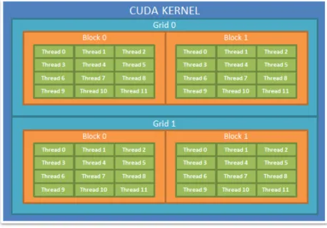
4.1 Example of CUDA kernel hierarchy. . . 26

4.2 Example of automatically scalability for 2 GPUs with different numbers of SMs. . 38

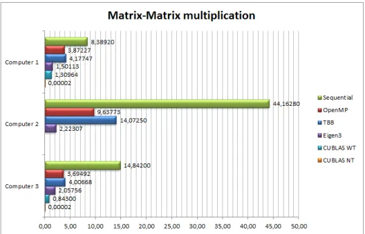
4.3 Matrix-matrix multiplication. . . 41

4.4 Matrix-vector multiplication. . . 42

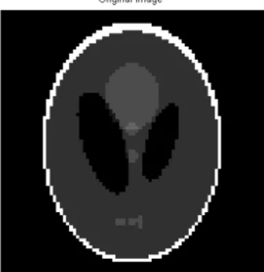
4.5 Shepp-Logan phantom original Image . . . 43

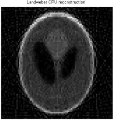
4.6 Shepp-Logan phantom Landweber reconstruction. . . 44

4.7 Shepp-Logan phantom ART reconstruction. . . 44

4.8 Shepp-Logan phantom Kaczmarz reconstruction. . . 44

4.9 Landweber method. . . 46

4.10 SART method. . . 47

4.11 Kaczmarz method. . . 48

5.1 Vertical layers of the Earth's atmosphere . . . 52

5.2 GPS signal between the satellites and receiver. . . 53

5.3 IWV, SIWV and Wet Gradient representation . . . 54

5.4 GNSS water vapor tomography. . . 56

6.2 Image created with PlotWaterVapor component in 43.25 latitude slice. . . 67

6.3 LOFTT_K 48.25 latitude slice. . . 68

6.4 SWART 48.25 latitude slice. . . 68

6.5 LOFTT_K 7.25 longitude slice. . . 69

6.6 SWART 7.25 longitude slice. . . 69

6.7 Convergence of SART algorithm for 1000 iterations. . . 70

6.8 Marseilles network area and receivers positions. . . 70

6.15 Belem network. . . 71

6.1 SWART UML component diagram. . . 73

6.9 SWART slice in latitude 43.25 for Marseilles network. . . 74

6.10 SWART slice in latitude 43.35 for Marseilles network. . . 74

6.11 SWART slice in longitude 5.35 for Marseilles network. . . 74

6.12 SWART slice in longitude 5.45 for Marseilles network. . . 74

6.13 SWART slice in height 500 for Marseilles network. . . 74

6.14 SWART slice in height 14500 for Marseilles network. . . 74

6.16 SWART slice in latitude -1.35 for Belem network. . . 75

6.17 SWART slice in latitude -1.45 for Belem network. . . 75

6.18 SWART slice in longitude -48.25 for Belem network. . . 75

6.19 SWART slice in longitude -48.45 for Belem network. . . 75

6.20 SWART slice in height 500 for Belem network. . . 75

(12)

(13)

List of Tables

4.1 Programming languages and applications programming interfaces supported by

the CUDA platform. . . 26

4.2 Computers Speci cations. . . 39

4.3 Matrix-matrix multiplication in the same computer with logical and physical pro-cessors. . . 40 4.4 Matrix-matrix multiplication. . . 40 4.5 Matrix-vector multiplication. . . 41 4.6 Shepp-Logan 80 x 80 - 50 iterations . . . 44 4.7 Shepp-Logan 50 x 50 - 50 iterations . . . 44 4.8 Shepp-Logan 80 x 80 - 1000 iterations . . . 45 4.9 Shepp-Logan 50 x 50 - 1000 iterations . . . 45 4.10 Shepp-Logan 80 x 80 - 10 000 iterations . . . 45 4.11 Shepp-Logan 50 x 50 - 10 000 iterations . . . 45 4.12 Landweber method. . . 45 4.13 SART method. . . 46 4.14 Kaczmarz method. . . 47

6.1 SlantDelayJoinProcessing Con guration File Options . . . 61

(14)

(15)

Acronyms

ART Algebraic Reconstruction Techniques BLAS Basic Linear Algebra Subprograms

CPU Central Processing Unit

CUBLAS CUDA Basic Linear Algebra Subroutines CUDA Compute Uni ed Device Architecture

DMA Direct memory access DOY Day Of Year

GNSS Global Navigation Satellite Systems GPS Global Positioning System

GPU Graphics Processing Unit IWV Integrated Water Vapor LAPACK Linear Algebra PACKage

LOFTT_K LOgiciel Français de Tomographie Troposphérique -version Kalman

OMP OpenMP

PC Personal Computer PPE Power Processor Element

SART Simultaneous Algebraic Reconstruction Technique SEGAL Space Earth Geodetic Analysis Laboratory

SIRT Simultaneous Iterative Reconstruction Techniques SIWV Slant Integrated Water Vapor

SMOG Structure of Moist convection in high-resolution GNSS observations and models

SPE Synergistic Processing Element

SWART SEGAL GNSS Water Vapor Reconstruction Image Software ScaLAPACK Scalable Linear Algebra PACKage

(16)

(17)

Chapter 1

Introduction

The algebraic reconstruction algorithms are iterative algorithms that were initially developed with success for medical imagery [1] although they are now used over other domains (e.g. medicine, seismology and meteorology). The data retrieved for the image reconstruction can be obtained from diverse sources such as X-ray, magnetic resonance imaging or seismic travel times. Algebraic reconstruction algorithms were rst described in [2] by Stefan Kaczmarz and were later rediscovered in the eld of image reconstruction from projections in [1] by Gordon

et. al. The algebraic reconstruction algorithms have some advantages over other inversion

algorithms, namely high numerical stability and computational ef ciency [3]. In [3] Bender et.

al successful applied the algebraic reconstruction technique for the water vapor reconstruction.

Water vapor plays an important role in the weather and climate phenomena such as rainstorms, thunderstorms and other strong convective weather events [4]. It is also important for precipi-tation forecast and nowcasting [5]. Therefore it is very important to measure the water vapor distribution and its variation in the atmosphere.

The signals of GNSS satellites must travel through the atmosphere in order to be received by the GNSS receivers. The atmosphere's atoms and molecules slow down the GNSS satellites signals [6] causing a delay. It is possible to separate the water vapor delay from other dry gases delays such as nitrogen, oxygen and carbon dioxide [6] and consequently estimate the water vapor in the atmosphere using GNSS.

The GNSS water vapor estimation has many advantages over other methods (e.g., radiosonde, satellite platforms using infrared, microwave sounders), such as good temporal resolution, it operates in all weather conditions and it can run unattended [7]. GNSS water vapor tomography (image reconstruction) was rstly described in [8] by Bevis et. al. The water vapor image can be reconstructed using the diverse slant wet delays of a GNSS receiver in the direction of the visible satellites1_{. There are several techniques to reconstruct the water vapor image in the}

atmosphere using the slant wet delays, including the algebraic reconstruction algorithms. Algebraic reconstruction algorithms are known to be highly computational intensive [9]. This fact may be troublesome if they are used for real time image reconstruction of GNSS water vapor elds, especially if processed in the conventional personal computers (PCs). Therefore, the improvement of the performance of the estimation is a critical issue on the implementation of these algorithms for water vapor tomography. Obviously the computational resources needed depend on the size of the reconstruction problem and this depends on the quantity of data available, satellites, receivers and slant wet delays, for instance in [3] large problems sizes (matrix with 26000 x 8280 elements) are generated.

1_{The slant wet delay consists in the delay caused by the water vapor in the satellite's signal mapped in}

(18)

1.1 Objectives

The main objective of this dissertation was to study the the parallelization of algebraic recon-struction algorithms in order to evaluate its potential advantages. Although the parallelized algebraic reconstruction algorithms can also bene t other research areas, a complementary goal was to investigate its application on the estimation of GNSS water vapor elds. Nowadays there are several GNSS water vapor image reconstruction software packages, however none of them implements parallelized algebraic reconstruction algorithms.

As consequence of this study, an application to perform the GNSS water vapor reconstruction using the algorithms and techniques developed was implemented: SWART (SEGAL GNSS Water Vapor Reconstruction Image Software). An additional objective of the development of this ap-plication was to implement it in conventional low cost personal computers taking full advantage of modern multicore and GPU architectures.

1.2 Main Contributions

The main contributions of this dissertation are here presented.

The rst contribution is the analysis of a range of parallel libraries and implementations for the linear algebra operations and consequently the parallelization of the algebraic reconstruction algorithms.

The second contribution consists in the development of a GNSS water vapor image reconstruc-tion applicareconstruc-tion that gathers all the necessary GNSS observareconstruc-tions and performs the correspon-dent water vapor image reconstruction. The software parameters are also customizable to the user.

During the course of this dissertation the following documents and conference papers were written:

An article with the title Analysis of algebraic reconstruction algorithms performance in CPU and GPU was submitted and accepted for the ICEUBI conference (http://iceubi2013.ubi.pt). A conference paper with the title A Study of GNSS Water Vapor Parameters was written and accepted as a presentation for the American Geophysical Union (AGU) 2013 Fall Meeting at San Francisco. This presentation will present an analysis of the various parameters to the GNSS wa-ter vapor reconstruction using the SWART program. Some of these paramewa-ters include covering diverse grid sizes and different number of receivers for the same water vapor image recon-struction. Also comparisons with LOFTT_K (LOgiciel Français de Tomographie Troposphérique -version Kalman) using synthetic data and results from Belem, Brazil which data was acquired in the framework of the project CHUVA will be presented. The AGU 2013 Fall Meeting website can be consulted in http://fallmeeting.agu.org/2013/.

A detailed technical report describing and comparing multithreading algebraic reconstruction algorithms was also written, Multithreading ART: Comparison 2_.

(19)

1.3 Dissertation Structure

The structure of this dissertation is here described. The current chapter contains the problem de nition, the principal objectives of this dissertation, the main contributions of this disserta-tion.

In Chapter 2 algebraic reconstruction de nition is de ned and techniques described.

Chapter 3 presents the state of the art of two main topics: GNSS water vapor tomography and algebraic reconstruction parallelization which consists in CPU, GPU and hybrid parallelization. Chapter 4 introduces the parallelization of the algebraic reconstruction, namely the approach used, the libraries tested and the parallel implementations and the results of these tests. In Chapter 5 the relation between the GNSS and the water vapor is described in more detail namely the de nitions and the methods of estimating water vapor and reconstructing its image. In Chapter 6 the GNSS water vapor image reconstruction software in development is presented. It is compared with another GNSS water vapor image reconstruction software named LOFTT_K and synthetic and case study results using the implemented software are presented and dis-cussed.

And nally in Chapter 7 the conclusions of this dissertation are presented and future work is described.

(20)

(21)

Chapter 2

Algebraic Reconstruction

Algebraic Reconstruction is an iterative approach for imaging reconstruction using data obtained from a series of projections such as those obtained from electron microscopy, x-ray photography and in medical imaging like in computed axial tomography (CAT scans). It consists of obtaining data from cross sections of an object from measurements taken from different angular positions around the object and then solving for an array of unknowns that represent the interior of the object being analysed. In Figure 2.1 we can see 6 line projections from three angular positions through an unknown object. For medical applications algebraic reconstruction algorithms lack the accuracy and speed of implementation when compared to other methods [10]. However there are situations where is not possible to measure a suf ciently large enough number of projections or when the projections are not uniformly distributed over 180 or 360 degrees, which prevents the use of other techniques such as transform based techniques that can obtain higher accuracy. The algebraic reconstruction algorithms also have the advantages of having high numerical stability even with inaccurate initial data and are also computationally ef cient and easily parallelized [3].

Algebraic techniques are also useful when energy propagation paths between the source and re-ceiver positions are subject to ray bending on account of retraction or when energy propagation undergoes attenuation along ray paths [10].

In the algebraic techniques studied in this dissertation is essential to determine the ray paths that connect the corresponding transmitter and receiver positions. When refraction and diffrac-tion effects are substantial it becomes impossible to predict ray paths which ends in obtaining meaningless results [10].

In this section the concept of algebraic reconstruction is introduced and the main algorithms are described.

2.1 Image and projection representation

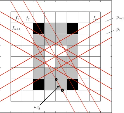
Consider a two dimensional image I = f(x, y). Figure 2.1 shows a square grid superimposed onto this image, we want to obtain this image from the projection data, shown as straight lines which traverse the (x, y) plane. We assume that for each cell f(x, y) is a constant and let fj : j = 1..N be the constant values for each cell of the image. N is the total number of cells

in the grid. A line integral will be de ned as array-sum. This ray sum is referred as pi, where i

is the i-ray.

(22)

Figure 2.1: Unknown image on square grid. Each cell value is a unknown variable to be determined using the various projections.

N

X

j=1

wijfj= pi, i = 1, 2, · · · , M (1)

M is the total number of rays (all projections), wij is the weight of the contribution of the jth

cell to the ith ray integral (this is proportional to fraction of the jth cell intercepted by the ith ray as shown in Figure 2.1).

Depending on the context many of the wij may be zero because only a small number of the wij

actually contribute to each ray-sum.

The equation in (1) can be rewritten in matrix form as follows:

Ax = b (2)

where A is a matrix with all the wij contributions, b is a vector with every pi ray sum and x is

a vector that contains all fj cells constant values (the original image). M and N correspond

respectively to the rows and columns of A.

If M and N were small one could use traditional matrix theory methods to invert the equation system of (1). In practice N may be large, for example for a 256 x 256 image N would be 65.536. If M had more or less the same value then for these values the size of the matrix [wij]

in (1) would be 65.536 x 65.536 which basically rules out any chance of direct matrix inversion [10].

(23)

Also when noise is present in the measurement data and M < N, even for relatively small N it is not possible to use direct matrix inversion. In this case one can use use a least square method to obtain an approximate solution, however when M and N are large these methods are computationally impracticable [10].

There are however some very attractive methods for solving these equations. These methods are based on the method of projections which Kaczmarz rst proposed [11]. First the equation (1) will be expanded to explain the computational procedure of these methods:

w11f1+ w12f2+ w13f3+ · · · + w1NfN = p1 w21f1+ w22f2+ w23f3+ · · · + w2NfN = p2 .. . wM 1f1+ wM 2f2+ wM 3f3+ · · · + wM NfN = pM (3)

A grid with N cells gives an image with N degrees of freedom. The image represented by (f1, f2, · · · , fN)can be seen as a single solution in an N-dimensional space.

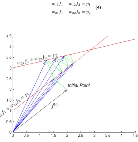
Each of the equations in (3) represents a hyperplane. When there is only one solution to the equations it is represented as a single point, namely the intersection of all the hyperplanes. This is the main concept that's illustrated in Figure 2.2. In this gure we have only considered two variables f1and f2 which satisfy the follow equations:

w11f1+ w12f2= p1

w21f1+ w22f2= p2

(4)

(24)

The computational procedure to calculate the solution is the following: 1. Start with a initial guess

2. Project the initial guess onto the rst line

3. Reproject the resulting point from 2 to the second line (3) 4. Reproject the result point from 3 to the rst line and so on 5. If there's a unique solution the algorithm will converge. The initial guess is written as(f(0)

1 , f (0) 2 , · · · , f

(0)

N ) or simply by the vector ~f

(0)_{. Often the initial}

vector is simply a zero vector. This vector is then projected onto the hyperplane using the rst equation on (3) resulting in the ~f(1)_{vector. This can be seen in Figure 2.2 for a two dimensional}

space. After that ~f(1) _{is projected by the second equation on (3) on the hyperplane resulting}

on ~f(2)_{and so on. In 2.2 the projections are the green lines and the blue vectors represent the}

next estimates of the solution.

When ~f(i−1) _{is projected on the hyperplane represented by the ith equation it can be}

mathe-matically be described as:

~ f(i)= ~f(i−1)−f~ (i−1)_{· ~}_w i− pi ~ wi· ~wi ~ wi (5)

where ~wi= (wi1, wi2, · · · , wiN)and ~wi· ~wiis the dot product of the vector ~wi by itself.

Regarding the algorithms convergence, it is easily seen that in the case of two perpendicular hyperplanes then for any initial guess in the (f1, f2)plane it is possible to nd the solution in

only two steps using (5). However if the two hyperplanes have a reduced angle between them there will be a greater number of iterations (depending also on the initial guess).

In fact if the M hyperplanes in (3) could all be made orthogonal (perpendicular) with respect to one another then the solution could be found in only one pass through all the equations in (3) (assuming that only one solution exists) [10].

This is theoretically possible using for example a method for orthonormalising a set of vectors such as the Gram-Schmidt procedure. However in practice it is not computationally viable as the orthnomalizing process itself takes too much time. Another problem with orthogonalization is that it ampli es the noise problem from the measurements into the nal solution [10]. If we have M > N in (3) no unique solution may exist, although a solution in a zone may still be determined. Figure 2.3 shows a two variable system with three noisy hyperplanes. In this case we see the result after projecting the initial point onto the rst line (in green) and then iterating 100 times, the gure show the projections onto the hyperplanes. As can now be seen the procedure in (5) does not converge to a unique solution but instead it oscillates in the neighbourhood of the intersections of the hyperplanes.

In the case of M < N a unique solution also doesn't exist, instead there are multiple solutions. For instance if we have only one equation of the two in (4) to calculate the two variables, then the solution can be on any point in the line that corresponds to this equation.

Another advantage of this method is the possibility of adding a priori information already known about the image being reconstructed in order to guide the solution. If we know for example

(25)

Figure 2.3: Case where the number of equations is greater than the number of unknowns and projections have been corrupted by noise.

that the image contains no negative values and if during the iterative process we obtain we some negative value one can simply reset those values to zero.

2.2 Techniques

There are two different techniques for algebraic reconstruction, namely: Algebraic Reconstruc-tion Techniques (ART) and Simultaneous Iterative ReconstrucReconstruc-tion Techniques (SIRT) which will be described in the follow subsections.

Different methods of these techniques namely Kaczmarz, Symmetric Kaczmarz, Landweber, Cimmino, CAV, DROP and SART which were implemented for this dissertation will now be pre-sented.

2.2.1 ART methods

The Algebraic Reconstruction Techniques (ART) are row-action methods that treat the equations one at time. This means that in each iteration each equation is solved individually. The updates in each ith iteration are made using the equation on (5) plus a relaxation parameter λkresulting

(26)

~ f(i)= ~f(i−1)+ λk pi− ~f(i−1)· ~wi ~ wi· ~wi ~ wi (6)

What distinguishes the various methods is the order in which row is processed [12]. The ART reconstructions usually suffer from so called salt and pepper noise, which is caused by the fact that the values of wijare only approximations as they are usually measured by experiments

[10].

2.2.1.1 Kaczmarz

This is the most well know ART method in the literature [13] [14]. It uses a xed λk= λ ∈ (0, 2)

in the original paper the value 1 was used. In the literature this method is also referred as ART which can give rise to some confusion since it is also used for Algebraic Reconstruction Techniques. Each kth iteration in Kaczmarz consists of one sweep in each row of A from the top to the bottom: i = 1, 2, ..., m.

2.2.1.2 Symmetric Kaczmarz

This method is a variant of the previous Kaczmarz method. It adds a new sweep using the rows in the reverse order. As result each kth iteration consists of 2 steps: i = 1, 2, · · · , m − 1, m, m − 1, · · · , 3, 2.

This method supports both a xed (λ ∈ (0, 2)) and iteration-dependent λk.

2.2.2 SIRT methods

The Simultaneous Iterative Reconstruction Techniques (SIRT) are simultaneous because all equations are solved at the same time in one iteration (based on matrix multiplications) [12]. Usually these methods converge slower to the solution than the ART methods, however they result in better looking images [10].

The SIRT methods work by rst solving all the equations and updating only the cell values at the end of each iteration. The change of each cell is the average of each of the changes for that cell [10].

The general form of these methods is as follows:

~

f(k)= ~f(k−1)+ λkT ATM (p − A ~f(k−1)), k = 0, 1, 2, · · · (7)

where A is the matrix with the various projections, λk is a relaxation parameter and the

ma-trices M and T are symmetric positive de nite. The various SIRT methods depend on these matrices. λk is de ned as 2/ρ(T ATM A) − ε, where ρ is the spectral radius, ε the machine's

(27)

Three of the SIRT methods presented here include positive weights ti> 0, i = 1, · · · , m. If the

weights are not speci ed then all the weights are set to 1. The methods that include these weights are Cimmino, CAV and DROP and will be presented below.

2.2.2.1 Landweber

The Landweber method is described by the following form: ~

f(k)= ~f(k−1)+ λkAT(p − A ~f(k−1)), k = 0, 1, 2, · · ·

which corresponds to replacing M = T = 1 in (7).

2.2.2.2 Cimmino's method

This method was rst introduced in [15] and it's often presented in a variant based on projec-tions. The version presented in this dissertation is the same from [12]. This version includes a relaxation parameter λkand also a weights vector ~t.

Using the matrix notation this method uses the equation (7) with M = D and T = I, where D is de ned as: D = 1 mdiag ti k ~wik2₂ ! (8)

2.2.2.3 Component averaging (CAV)

Cimmino's original method uses equal weighting of the contributions from the projections, which looks fair when A is a dense matrix [12]. The CAV method was introduced in [16] as an extension to the Cimmino's method to take in account the sparsity information in a heuristic away [12]. Let sj be the number of nonzero (NNZ) elements of column j:

sj =NNZ(aj), j = 1, · · · , n (9)

Also de ne the diagonally matrix S = diag(s1, · · · , sn) and the norm k ~wik 2

S = ~wi · S ~wi =

Pn

j=1wijsj for i = 1, · · · , m.

Using the matrix notation this method uses the equation (7) with M = Dsand T = I.

Dsis de ned as: Ds=diag ti k ~wik2_S ! (10)

(28)

2.2.2.4 Diagonally Relaxed Orthogonal Projections (DROP)

DROP is another Cimmino's extension. Using the matrix notation it uses the equation (7) with T = S−1, M = mD. The matrix D is from (8) [12].

In [17] it is proved that ρ(S−1_AT

M A) 6 maxi{ti}, this means that the convergence is

guaran-teed if λk 6 (2 − ε)/maxi{ti}

2.2.2.5 Simultaneous Algebraic Reconstruction Technique (SART)

These methods were originally implemented as ART methods [18], but can also be implemented as SIRT method. They are described by the following :

~

f(k)= ~f(k−1)+ λkD−1r A T_D−1

c (p − A ~f

(k−1)_), _{k = 0, 1, 2, · · ·}

D−1_r and D−1_c are diagonal matrices corresponding respectively to the row and column sums:

Dr= diag(|| ~wi||1) Dc = diag(|| ~wj||1).

where ~wj= (w1j, w2j, · · · , wN j).

There's no need to include weights in this method as the convergence for this method was established in [19] [20] and it was shown that ρ(D−1

r ATDc−1A) = 1.

2.3 Summary

In this chapter an overview to algebraic reconstruction was realized. It was described the main advantages and applications of these techniques. The two different categories of algebraic reconstruction were presented (ART and SIRT) and some methods of each category were also described. The current chapter is important as basis to the reader understand the following chapter which will present the state of the art of GNSS Water Vapor Tomography and Parallel Algebraic Reconstruction Algorithms.

(29)

Chapter 3

State of the Art

In this chapter the state of the art of the water vapor tomography plus the parallelization of the algebraic reconstruction algorithms will be presented. The parallelization of the algebraic reconstruction algorithms will consist in a brief overview of the various implementations namely the cpu implementation, gpu implementation and the hybrid cpu/gpu implementation. This chapter is organized by topic and inside each topic it is organized chronologically.

3.1 GNSS Water Vapor Tomography

GNSS Water Vapour tomography is a technique that allows the distribution of the water vapor on the atmosphere to be calculated [21][22][5].

The calculation of the water vapor is and remains dif cult to quantify due to the high variability in time and space plus the sparse set of available measurements [21].

The GPS was proved to measure the integrated water vapor at zenith with similar accuracy as other methods such as radiosondes [23] or water vapor radiometers [24][25]. Also compared to water vapor radiometers the GPS operates in all weather conditions without the need of dif cult calibration procedures [21]. Studies have shown that it is possible to quantify the inte-grated water vapor on the line of sight of the GPS satellite [26] [27] [28]. This quanti cation is designated as slant integrated water vapor (SIWV) [21] and they are used to calculate the water vapor distribution. Water vapor is a key item in numerical weather prediction, since it plays an important role in atmospheric processes, especially precipitation forecast and nowcasting, hazard mitigation and water management [22] [5]. In the last years, the development of tomo-graphic methods to calculate the 3D distribution of water vapor in the troposphere has been a main topic of research [29].

In [30] Michael Bevis et al. showed how to map zenith wet delays onto precipitable water (PW) with an root mean square (r.m.s) error less than 2 mm + 1% of the PW and long-term biases of less than 2 mm.

Niell has introduced in [31] two new mapping functions denominated as Niell Mapping Functions (NMF). These functions are used to map a zenith delay in elevations angles down to 3◦_{. The}

rst function is an hydrostatic mapping function which depends on the latitude, the height of the receiver and the day of year (DOY)

A. Flores et al. have shown in [32] how GPS data are processed to obtain the tropospheric slant wet delays. It was con rmed that the tropospheric tomography is a practical approach to the description of the spatio-temporal structure of the water vapor in the atmosphere. In [32] the software LOTTOS for obtaining the tomographic solution using data from Kilauea network, Hawaii in 1 February, 1997 is described.

(30)

In [33] John Braun and Christian Rocken used slant water observations as input into a tomog-raphy software based on the algorithm used at [32]. In [33] the linear system is solved using singular value decomposition on the original observation-state matrix without computing the normal equations. This method improved the sensitivity of the solution and allowed a more accurate determination of the water vapor.

Ulrich Foelsche and Gottfried Kirchengast developed in [34] a two dimensional, height-resolving tomographic imaging technique following the Bayesian approach for optimal combination of the information from different sources. This water vapor imaging technique combines ground based line integral measurements with an occultation pro le which uses optional estimation. The authors mentioned that the occultation could be replaced by other pro le data like radiosondes. The image algorithm was tested using simulated data. It was concluded that the technique is capable of reasonably reconstructing realistic atmosphere features. It was also concluded that areas with high absolute humidities and small-scale variations of water vapor density usually result in images of good quality.

In [35] LOTTOS software from [32] was used in a small scale GPS campaign (seven GPS receivers distributed within a 3 km radius). To calculate the inversion of the data collected it was used the singular value decomposition (SVD) technique described in [36]. The tomographic results were compared with radiosonde data and the agreement between the solutions was shown to be good. It was concluded that tropospheric tomography is reliable even with a reduced number of stations and that tomography is a potential tool to describe the spatio-temporal structure of the refractivity.

In 2005 a campaign denominated ESCOMPTE was used in [21] to run a GPS experiment. This GPS experiment had the following objectives: to estimate the integrated water vapor (IWV) in conjunction with the atmospheric dynamics, the study of the GPS-retrieved horizontal gradients and the development of tomography for three-dimensional reconstruction of the atmospheric humidity eld. The campaign used 16 stations over the urban and northern border of Marseille within a area of approximately 20 x 20 km. Additional observations were also acquired using other type of systems: a water vapor radiometer, a solar spectrometer and a prototype water vapor Raman LiDAR. These instruments allowed independent IWV measurements for comparison and validation of the GPS results. The results of three inversions in [21] were shown to be consistent when compared with three radiosondes launches. The ESCOMPTE campaign provided the important data for the successful inversions, namely ZTD and horizontal gradient volumes of sight of the GPS satellites which were used for the calculations of the SIWV values used in the tomography.

An alternative approach to estimate the three-dimensional structure of the water vapor was presented in [37]. It uses the raw GPS phase observations. More speci cally, instead of using one model for the slant delays in the GPS processing and another for the calculation of wet refractivity eld, the voxel discretization of the wet refractivity in the GPS processing step is applied. The advantages of this method include that any error in the modelling of the slant wet delays in terms of zenith delays and gradients will disappear and that the number of steps required to obtain the wet refractivity eld is reduced. The disadvantage is that there are many parameters that need to be estimated in the processing. The results have shown that having a spread in the station heights and using more than one GNSS will improve the retrievals of the refractivity elds. The results also indicate that the refractivity eld can be obtained with an accuracy of approximately 20% or better to around 4 km with a height resolution of 1

(31)

km (provided that there are enough number of satellites and stations).

Troller et al. developed in [38] the software package AWATOS (atmospheric water vapor to-mography software). This software is based on the assimilation of double differenced GPS observations. AWATOS applies a least-squares inversion to reveal the inhomogeneous spatial distribution of water vapor. Using this software an extensive investigation has been carried out in Switzerland using the national AGNES GPS network. For validation, 22 radiosondes pro les and the numerical weather model aLMo (alpine model in Switzerland, MeteoSwiss) were used to compare with the tomographic results. An overall goal agreement was achieved between the three methods with an root mean square (r.m.s) of better than 1.6g/m3_{absolute humidity.}

Miidla et al. have presented in [39] an overview of some mathematical methods for detection, monitoring and modelling of the tropospheric water vapor. It was concluded that the modelling environment works well for receiver-network geometry analysis. To nish Peep Miidla et al. conclude that future work will focus on data ltering and how to improve the poor voxel ge-ometry in an optimal way, since they believe to be key issues in the construction of effective GPS-receiver networks for water vapor tomography.

Bender et al. developed a GNSS water vapour tomography system in [3] to reconstruct spatially resolved humidity elds in the troposphere. This system was designed to process the slant delays of about 270 German GNSS stations in near real-time with a temporal resolution of 30 minutes, horizontal resolution of 40 km and a vertical solution of 500 m or better. For the inver-sion Michael Bender et al. implemented different iterative algebraic reconstruction techniques (ART) comparing them with respect to their convergence and some numerical parameters. It was found that the multiplicative techniques (MART) provided the best results with the least time [3]. It was also found that noise added to data didn't disturbed the ART algorithms too much as long the noise did not exceed 50% of the SWV. This is a good feature since other inverse techniques often produce meaningless results over noise addition. The authors concluded that the iterative techniques were successful used in the GNSS tomography and could be parallelized to run on multicore processors or computer clusters.

In [22] Perler et al. introduce two new parametrizations of voxels in the Kalman lter-based GPS tomography software AWATOS 2 and their treatment in ellipsoidal coordinates. Also inter voxel constraint are presented. The ability of these parametrizations to reconstruct a four-dimen-sional water vapour eld with high quality was demonstrated. These algorithms showed how to reduce the discretization effects without signi cantly increasing the number of parameters estimated. The tests performed indicated good performance of the parameterized algorithms. The accuracy increased about 10-20% for simulated data. Besides the simulations, data were also acquired from 40 GPS stations. The results using the real data also showed better per-formance compared to the non parameterized approach. The authors highlight that for future investigations the focus should be in the evaluation of longer periods and on comparisons with additional quantities like zenith wet delays.

3.2 CPU Algebraic Reconstruction Algorithms Parallelization

In this section we present some of the algebraic reconstruction algorithms that have been parallelized in recent years using multi-processors (CPU's).

(32)

Melvin et al. designed and developed a parallel ART algorithm (PART) in [40]. Its performance was studied for a network of workstations using the Message Passing Interface (MPI). In the algorithm implemented the projections data (e.g. delay between source and receptor) are partitioned and distributed over all processors. For each projection data of a processor, the reconstruction projections are calculated, it is also calculated an adjustment vector and the adjustments are applied to the image being reconstructed. In the last step the algorithm normalizes the images values. The major bottleneck in the algorithm was said to be caused by the communication time between processors.

In [41] a method to speed up a 3D simultaneous algebraic reconstruction technique using MPI was proposed using a parallel programming method on a computer cluster system. The amount of work is distributed to each computer node using a centralized dynamic load balancing and a work-pool scheduling scheme. This method was considered to be simple, fast and highly effective. The time cost of the reconstruction process decreases as the number of processing nodes increases. Four nodes accelerated the process 4.55 times when comparing with the sequential implementation. Also the proposed system decreased the reconstruction times up to 78% percent when comparing with a normal image reconstruction form projection in a single computer [41].

Gordon has shown in [42] that ART can be parallelized on a linear processor array. It was demonstrated that the reconstruction of an image of n pixels using Θ(n) equations can be done on a linear array of p = O(√n)processors with optimal ef ciency (linear speed up) and O(n/p) memory needed for each processor. This ART parallelization uses linear and rectangular arrays of processors which are also known as meshes. In this systems each processor is only connected directly to a small and xed number of neighbouring processors. This PART implementation can be applied to various geometric models of image reconstruction and be extended to spherically symmetric volume elements (blobs) instead of voxels [42].

A tomographic reconstruction software, developed using Adaptive MPI (AMPI), was presented in [43]. AMPI is a user level thread framework that provides a solution to port legacy MPI code into a multithreaded environment where overlapping is possible (do not block objects involved in the communication).

In [43] the block iterative of component averaging methods, BICAV, has been parallelized using the Single Program Multiple Data (SPMD) approach. The volume being reconstructed is divided into slabs of slices. The slabs of slices will be distributed over the processes (MPI) or virtual processes (AMPI) for the parallelization. In MPI approach communication between the various computer nodes is involved and reducing latency becomes an issue. The AMPI library permits latency reduction using the computation-communication overlapping. In the same CPU while one thread is waiting, another one can progress with the application. Some tests were realized to compare the differences between the BICAV parallel implementation in both MPI and AMPI. The results have shown that for AMPI the walltime and cputime are almost the same while in MPI their differences may be signi cant, especially when increasing the number of processors. It was concluded that the threaded version of BICAV (AMPI) scales signi cantly better than the MPI version [43] and therefore concluded that user level threads are an attractive method for parallel programming of scienti c applications.

Melvin et al. had examined the ef ciency of the parallel ART on a shared memory machine on the Western Canada Research Grid Consortium [9]. Two algorithms using multithreading on the shared memory machine were implemented. OpenMP library were used for the parallel

(33)

implementation. Some tests were also executed to time the performance of the parallel al-gorithms. The results have shown a clear advantage with a greater number of threads. With the increasing of the number of processors the speed up also increased, with ef ciency ranging from 59.52% to 96.75% [9]. A six processor IBM P-server reconstructs an image from 36 angles in approximately 5.038 seconds, with an ef ciency of 93.35%. This means that a parallel ART algorithm can reconstruct the same image, in about the same time as a 180 angles sequential FBP (Filtered Back Projection) reconstruction, with about the same image quality and less radi-ation. With the same radiation the 5.038 parallel algorithm produces a higher quality image in approximately the same time [9].

In [44] a Modi ed Simultaneous Algebraic Reconstruction (MSART) was implemented. This algo-rithm implements a back projection technique (BPT) and an adaptive adjustment of corrections. The experimental results have shown that MSART can improve signi cantly the quality of recon-struction. A strategy to parallelize the MSART algorithm on DAWNING 4000H cluster system were also implemented. The parallelization of MSART has made for 3D volumes on cluster systems. Basically the 3D reconstruction problem is decomposed into a set of independent 2D reconstruc-tion problems. The algorithm combines both MPI and OpenMP libraries. The MPI library is used to perform the coarse-grained parallelization of the reconstruction. OpenMP is used to perform the ne-grained parallelization [44]. This hybrid implementation has proven to be better than only the MPI one [45]. In the algorithm each slabs of slices is assigned to an individual node in the cluster and the reconstruction is made in parallel. The nodes communicate with each other only to complete the nal result of the 3D reconstruction [44]. The results have shown that the speedup decreases with the increasing of the number of computer nodes. This is justi ed by the increase of the communication time between the nodes since the number of nodes also increase [44]. Overall the results on DAWNING 4000H cluster system show that the implemented 3D reconstruction parallel algorithm can achieve high and stable speed ups [44].

Xu and Thulasiraman have implemented a parallelized ordered subset [46] SART (OS-SART) on cell broadband engine [47]. The algorithm takes advantage of Cell BE architecture, using the SPEs (Synergistic Processing Elements) coprocessors to compute the ne grained independent tasks and PPE (Power Processor Element) performs the tasks of data distributing and gathering. The overlap of the computation and communication is realized with direct memory access available on the Cell BE, this to reduce the synchronizing and communications overheads [47]. The algorithm consists in four parts: forward projection, rotating the image, back projection and creating the reference matrix. The algorithm has tested in two different architectures: Cell BE and Sun Fire x4600. The more time consuming parts of the algorithm are forward and back projections the total complexity of the algoritm is O(n3₎ _{which turns the OS-SART}

in a computation intensive algorithm. This algorithm is also memory intensive consisting in a complexity of O(n4₎_{[47]. Cell BE is a PowerXCell8i within a IBM QS22 Blade. This computer runs}

at 3.2 GHz and contains 16 GB of shared memory. The sun re x4600 machine is a distributed shared memory system with an eight AMD dual-core opteron processor resulting in a total of 16 cores. Each core runs at 1 GHz with 1 MB cache per core and 4 GB memory per processor. In this system OpenMP was used for the implementation. A series of tests were realized in [47] comparing the execution time, number of subsets, number of cores, number of SPEs and the number of images rows per DMA (Direct memory access) transfer. The tests have shown that one drawback of the Cell BE is the limited memory storage on each of the SPEs. The approach the authors used to circumvent this problem were to use a rotation based algorithm which calculates the projection angles using less memory. However this rotation based algorithm

(34)

increases the number of transfers required to DMA from main memory to local memory on the SPE, which turned to be a bottleneck how the number of SPEs increased. Even with this bottleneck the Cell BE performed much better than the shared memory machine [47]. The tests also exposed that the number of subsets impacts the sequential processing time on one SPE. The Cell-based OS-SART on one SPE was ve times faster than OS-SART on AMD opteron core for one subset and one iteration. With the increase of the number of subsets the speedup also increased. The authors referred that a future implementation the algorithm will use double buffering, in order to reduce the DMA transfers impact.

3.3 GPU Algebraic Reconstruction Algorithms Parallelization

Algebraic reconstruction algorithms are highly computational intensive. With this in mind var-ious hardware platforms have been tested along the years including the Graphics Processing Units (GPUs) discussed in this section.

In 2000, Klaus Mueller and Roni Yagel made an implementation in OpenGL of the SART recon-struction technique using 2-D texture mapping hardware in [48]. This implementation was used for rapid 3-D cone-beam reconstruction. It was found that the graphics hardware allowed 3-D cone beam reconstructions with speed ups of over 50 comparing with the implementation on a epoch's CPU. The graphics hardware version of SART developed was named texture-map-ping hardware accelerator SART (TMA-SART). Both the software implementation (SART) and the hardware implementation (TMA-SART) used as test image the 3D-extension of the Shepp-Logan phantom [49]. The projections were obtained by analytical integration of the phantom and were used to reconstruct a 1283 _{volume in three iterations. Two graphic architectures groups}

were used in the experiments: an epoch's mid-range workstation, such the SGI Octane with a 12-bit framebuffer and low-end graphics PCs and graphics boards that only had a 8-bit frame-buffer. The experiments indicated that the rst group had speed ups between 35 and 68 when compared to an optimized CPU version of the SART algorithm (in the same system CPU) [48]. In 2005, Fang Xu and Klaus Mueller have shown in [50] how the PC graphics board technology had an enormous potential for the computed tomography. The authors decomposed three pop-ular three-dimensional (3D) reconstruction algorithms (namely Feldkamp ltered backprojec-tion, the simultaneous algebraic reconstruction technique and the expectation maximization) into modules which could be executed on the CPU and their output linked internally. As an added bonus the visualization of the reconstructions is easily performed since the reconstruc-tion data are stored in the graphics hardware, which allowed to run a visualizareconstruc-tion module at any time. Several tests were performed on the three algorithms developed, the Feldkamp ltered backprojection, the simultaneous algebraic reconstruction technique and the expecta-tion maximizaexpecta-tion. This test were performed on a 2.66 Ghz Pentium PC with 512 memory and a NVIDIA FX 5900 GPU. A 3D version of the Shepp-Logan phantom with size of 1283 _{was used}

for the reconstruction tests. The results have shown that the epoch's inexpensive oating point GPUs could reconstruct a volume with SART in about 12 times faster than the same generation CPUs and ve times faster than the older SGI hardware [48]. It was noticed that the projections were much faster than the back projections. The authors concluded that the GPU implementa-tion of Feldkamp FBP produced excellent results. The GPU Feldkamp FBT reconstrucimplementa-tion was seen to be very fast taking 5 seconds to reconstruct a 1283 _{volume with good quality. The}

(35)

au-thors stated that for the rst time the quality of the GPU reconstruction could rival that of the CPU implementations. Also excellent GPU performance could be achieved in relatively cheap equipment ($500 for the epoch's).

Keck et al. have applied in 2009 the Common Uni ed Device Architecture (CUDA) to the SART algorithm in [51]. Two different implementations were made one using CUDA 1.1 and another using CUDA 2.0. Until this implementation the iterative reconstruction on graphics hardware used OpenGL and Shadding languages [50] [48]. With CUDA is possible to use the standard C programming language to program in a graphics hardware without any knowledge of graphics programming [51].

The back projection component of the SART algorithm performs a voxel-base back projection. The matrix-vector product is calculated for each voxel to determine the voxel corrective pro-jection value.

The forward projection is parallelized using each thread to compute one corrective pixel of the projection. In both the back and forward projection the CUDA grid sizes is chosen based on experimental results [52].

After the implementation of the SART in the GPU (CUDA 1.1 and CUDA 2.0) and in the CPU some experiments were made to evaluate the performance of each method. The GPU used for the experiments were a NVIDIA Quadro FX 5600. For the CPU two different hardware were used: an Intel Core2Duo 2 GHz PC and a workstation with two Intel Xeon Quadcore 2.33 GHz. The image used for the reconstruction had a size of 512x512x350 [51].

Using CUDA 1.1 the implementation took approximately 1.15 seconds for a single texture update [51]. Using 3D textures the authors measured 0.11 seconds for the texture update on CUDA 2.0 which improves the performance by a factor of 10 [51].

The slowest GPU SART implementation revealed to be CUDA 1.1 even so it still was 7.5 times faster than the PC and 1.5 times faster than the workstation. Ordered subsets [46] optimiza-tions in GPU had also been tested allowing even faster CUDA implementaoptimiza-tions. The CUDA 2.0 implementation with the ordered subset was 64 and 12 times faster compared to the PC and workstation respectively.

The authors concluded that GPU-OS CUDA 2.0 implementation was already applicable for spe-ci c usage in clinical environment, since this reconstruction was less than 9 minutes [51]. In [53] is presented some comparisons between GPU and CPU implementations of some itera-tive algorithms are presented: Kaczmarz's, Cimmino's, component averaging, conjugate gra-dient normal residual (CGNR), symmetric successive overrelaxation-preconditioned conjugate gradient and conjugate-gradient-accelerated component-averaged row projections (CARP-CG). Elble et al. have made a preliminary search to nd the most appropriate algorithms to be implemented in the GPU [53]. It became clear that the Kackzmarz algorithm was not the most appropriate, the only available steps that can be parallelized are the dot product and the vector addition. Due to this it could only be superior in terms of performance when using very large and dense linear systems. The BLAS library was used in the GPU for this hardware paralleliza-tion. It parallelizes the algebra operations like matrix-matrix or matrix-vector multiplications. The authors have made a series of tests using the various algorithms implementations both on CPU and GPU. The GPU implementations were processed on a NVIDIA Tesla C870 system and the CPUs implementations on a PC with a pentium IV 2.8 GHz processor with 1 GB memory. Also a

(36)

linux cluster with 16 of this PCs connected by a 1 Gbit/s Ethernet switch were used [54]. The results have shown that CGNR was the most ef cient algorithm for solving investigated partial differential equations on the GPU. The CAV algorithm highest GFLOPS but its slow convergence resulted in the slowest solution time [53]. The GPU had a clear advantage over the CPU, with computational results from ve to twenty times faster than the CPU. On the 16 node cluster the GPU implementation was up to three times faster [53]. As conclusion the authors mentioned that the GPU offered a low-cost and high-performance computation system to solve large-scale partial differential equations [53].

In [55] some benchmarks tests were realized to determine the optional parameters in the itera-tive algorithm OS-SIRT. The tests were processed on NVIDIA 8800 GT GPU and were programmed GLSL. This tests showed to be decisive for obtaining optimal GPU performance also they show that iterative reconstruction is a clear option for noisy and few-view scenarios.

Johnston et al. presents an implementation of family of iterative reconstruction algorithms with total variation (TV) denoising on a GPU (NVIDIA Geforce GTX 280). A series of tests to optimize and compare the ef ciency of each algorithm to reduce the artefacts were also ex-ecuted using a generated 2563 _{volume image. The results have shown that SART can achieve}

better performance than other implementations, namely steepest descent (SD) and the non linear conjugate gradient algorithm (CG).

In [56] implements the SART algorithm with motion compensation for a fast high quality com-puted tomography reconstruction using a CUDA GPU. Several tests were made to the imple-mented algorithm in order to test its performance, reconstruction quality and effect of the parameters. These tests were performed on a desktop PC composed of a Core2Quad Q6600 CPU (2.4 GHz), 4 GB memory and a NVIDIA 8800 GTX GPU with 768 MB ram and CUDA 2.0 [56]. The Shepp-Logan Phantom was chosen as the image to be reconstructed with a grid size of 1283

voxels and from a set of 80 projections. The CPU implementation took nearly 18 minutes to do the reconstruction while the GPU implementation took 7.52 seconds for ten iterations being almost 150 times faster than the CPU implementation [56]. The quality of the reconstruction this was evaluated using peak signal-to-noise ratio (PSNR), line pro les, visually and with met-rics like signal-to-noise ratio (SNR) and Mean Square Error (MSE). All this evaluations revealed satisfactory results [56]. The authors concluded that this SART GPU implementation allows instantaneous presentation of 3D CT volume to physicians once the projections are collected [56].

A distributed multi-GPU system (CUDA) was developed in [57]. The stated aim was to provide computing power for rapid constrained, iterative reconstruction of very large volumes. Shawn Q. Zheng et al. performed diverse tests with a system composed of 5 nodes where each node contained one GTX 295 card. Each GTX 295 card contains 2 GPUs resulting in a system composed by 10 GPUs. This system was connected using a high speed gigabit Ethernet network. For 10 iterations of SIRT reconstruction using a tomogram of 40962 _{x 512 from a input tilt series}

containing 122 projection images of 40962 _{pixels (using single precision) took a total of 1845}

seconds of which 1032 seconds are pure computation while the remainder are from the system overhead. The same distributed multi-GPU system took only 39 seconds to reconstruct 10242 _x

256 voxels from 122 10242 _{pixel projections. The authors concluded in [57] that even with the}

additional system overhead the performance analysis indicated that adding extra GPUs would improve the overall performance.

(37)

CUDA technology for the improved performance.

The implementation in CUDA uses a rotation technique involving 2D texture fetching [60] in order to reduce the memory usage. Two roughly independent stages are included in the bilinear rotation algorithm. One its the calculation of the exact coordinates on the source image and another it's the bilinear interpolation of the value over this point [58].

The authors have realized some tests for performance comparison and reconstruction quality comparison with the Filtered Back Projection (FBP) method. For this tests was used a PC with 2 AMD Opteron 275, 8 GB memory, NVIDIA GTX 285 with 240 cores executing Ubuntu Linux 9.10 64 bit as operating system. It was used double precision for the computations and Shepp-Logan phantom as image to reconstruct.

For a image of size 1500x1500 the CUDA implementation obtained a speed up of 6.6 relatively to the CPU implementation.

For the quality test a scanline of the reconstructed phantom was used, in this graph it is possible to see that the RegART is superior to FBP, resulting in fewer uctuations of the abortion coef cient [58].

The authors concluded that the CUDA RegART algorithm allows its use in real tomography hardware while further optimization would be a plus to compete with FBP in computational ef -ciency.

In [61] it is demonstrated that making alternative design decisions in the GPU implementation could result in an additional speed up of an order of magnitude comparing with the Xu et al. implementation [62]. It is mentioned in [61] that as the bandwidth available for reading data from the GPU global memory it is necessary to make use of the shared memory and cached mem-ory, even if it requires extra synchronization or memory writes. This especially important since tomography algorithms are very memory-read intensive. The projection and back projection are the steps more computational intensive so they were optimized using diverse techniques that exploit the memory locality. Same tests were carried to compare this implementation with Xu et al. implementation on [62]. In this tests two different generations of NVIDIA GPUs were used. A GTX 280 Geforce which contains a GT 200 GPU and was launched in 2008. This is the same GPU used by Xu et al. in [62]. The other generation used consisted in a Geforce GTX 480 and a Tesla C2070 both containing a Fermi GPU and launched in 2010. The results have shown that the optimizations that exploit the memory locality had an important impact on the running time of the projection and back projection steps of the GPU algorithm. Also a speed up of about 10 was obtained comparing with the results in [62] by Xu et al. using similar hardware [61].

3.4 Hybrid CPU and GPU Algebraic Reconstruction Algorithms

Parallelization

Besides the CPU and GPU only implementations for the algebraic reconstruction other hybrid solutions have emerged using both of this hardware.

In [63] a hybrid approach is presented that takes full advantage of the whole computer power available in modern computers and that further reduces the processing time. This approach

(38)

makes the decomposition of a 3D reconstruction problem into a set of independent 2D recon-struction subproblems corresponding to the slices perpendicular to the tilt axis. In this imple-mentation the slices are clustered in slabs of four slices to reduce the latencies and overheads. A pool of slabs to reconstruct is distributed over CPU (C-threads) and GPU (G-threads). As the threads become idle they are assigned to a new slab to reconstruct, the process is repeated until all slabs are processed. The authors explain in [63] that because GPU computation is much faster than in CPU more slabs are assigned to the GPU threads than to CPU threads. The authors also stated that for GPU was used a matrix approach (introduced in [64] that uses sparse struc-tures to improve performance) of the iterative methods while in CPU it was used a vectorized and optimized implementation (taking advantage of SSE, Streaming SIMD Extensions).

The results in [63] have show that the hybrid approach improves the performance over 1.5 to 2 times when comparing with strategies based on pure CPU or GPU implementations.

Another hybrid approach was presented in [65], this approach besides the CPU and GPU hard-ware also includes a eld-programmable array (FPGA). Here a new iterative reconstruction algorithm based on expectation maximization and total variation nominated as EM+TV is de-scribed.

In [65] the performance of the proposed hybrid architecture revealed to be the best when comparing with CPU and GPU only architectures. This architecture also delivers the minimum energy consumption, resulting in less than 1/3 of the CPU only implementation and 1/5 of the GPU only implementation.

3.5 Summary

In this chapter the state of the art of GNSS Water Vapor Tomography and Algebraic Reconstruc-tion Algorithms ParallelizaReconstruc-tion was presented. This chapter was important to understand what was been done in these areas and which approaches were followed. In the next chapter the work done in this dissertation will be presented for the parallelization of the algebraic recon-struction algorithms.

(39)

Chapter 4

Parallelizing Algebraic Reconstruction

One of the main objectives of this dissertation was to accelerate the algebraic reconstruction algorithms reducing their processing time and thereby permitting real-time applications. Alge-braic algorithms consist in a series of linear algebra operations as presented in Chapter 2. If we parallelize these algebra operations we automatically parallelize the algebraic reconstructions algorithms. This was the approach used in dissertation for the parallelization of the algebraic reconstruction algorithms. The linear algebra operations parallelized were the vector-matrix operation and the matrix-matrix operation. The programs were written and tested in regular personal computers (pcs) which are accessible to every user.

4.1 Multi-threading Libraries

There are several multithreading libraries for C++. The most elemental approach is to use a low threading library such as Pthreads (Posix Threads) or Boost, common higher level libraries are OpenMP and Intel Threading Building Blocks (TBB) [66]. This work aims to use and then compare the popular OpenMP and TBB libraries, since they provides a high level of abstraction of the implementation and platform plus they are known to be stable [67].

4.1.1 OpenMP

OpenMP (OMP) is a collection of compiler directives, library routines and environment vari-ables for shared-memory parallelism in C, C++ and Fortran programs. OMP is managed by the non-pro t organization OpenMP Architecture Review Board whose members include: AMD, Fu-jitsu, HP, IBM, Intel, Microsoft, NEC, NVIDIA, Oracle Corporation, Texas Instruments and others [68]. The OMP API requires that the programmer explicitly write the actions to be taken to ex-ecute the program in parallel. While aiding the coding when compared to lower level API's by introducing a high level of abstraction, it is not an automatically parallel programming model. OMP doesn't check for data dependencies therefore con icts such as race conditions, deadlocks and other multithreading problems may still occur [69]. It is up to the programmer to ensure correctness and deal with these speci c problems. OMP supplies primitives for locks and other multithreading primitives. OMP is included in many compilers by default including (but not limited to) GCC, XL C/C++ / Fortran, Visual Studio 2008-2010 C++ and nagfor [70].

An example of the OMP library is the following extracted code from the multiplication algo-rithm:

(40)

Listing 4.1 Example of use of the OMP library

1 #pragmaomp parallelfor

2 for(inti=0; i<M1−>rows−1;i+=2){ 3 intk; 4 register doubles00,s10; 5 s00=s10=0.0; 6 for(k=0;k<M2−>rows;k++){ 7 s00 += M1−>theMatrix[i] [k] v1[k]; 8 s10 += M1−>theMatrix[i+1][k] v1[k]; 9 } 10 result−>theMatrix[i] [j] =s00; 11 result−>theMatrix[i+1][j] =s10; 12 }

Notice the #pragma omp parallel for directive which automatically parallelize the for loop using the library.

4.1.2 Intel Threading Building Blocks

Intel Threading Building Blocks (TBB) is another library that helps the programmer write par-allel programs that take advantage of multicore processors that is also portable and scalable. Using TBB the programmer may build general purpose parallel programs and doesn't require any special languages or compilers. It is based on the use of C++ templates aiming to be si-multaneously exible and ef cient. TBB contains parallel algorithms and data structures it also provides scalable memory allocation and task scheduling [71].

The library uses tasks instead of threads and it internally maps the tasks onto threads [72].

TBB according to [72], was built with performance in mind, allowing computational intensive work parallelization. TBB is also compatible with other thread packages (for instance it is possible to write mixed OMP and TBB code).

An example of implemented code is given below which implements the same vector-matrix multiplication algorithm as was used for the OMP example (the details of dealing with the cases when the number of rows is odd are not shown):