Geoscientiic
Geoscientiic
Geoscientiic
Geoscientiic
1Dept. of Atmospheric and Oceanic Sciences, School of Physics, Peking University, Beijing, China
2Aviation Meteorological Center, Air Traffic Management Bureau, Civil Aviation Administration of China, Beijing, China
Correspondence to:B.-R. Wang (markwangpk@gmail.com)
Received: 12 October 2012 – Published in Atmos. Meas. Tech. Discuss.: 23 November 2012 Revised: 20 March 2013 – Accepted: 30 March 2013 – Published: 29 April 2013
Abstract.The radio occultation retrieval product of the Con-stellation Observing System for Meteorology, Ionosphere, and Climate (COSMIC) Radio Occultation sounding system was verified using the global radiosonde data from 2007 to 2010. Samples of 4 yr were used to collect quantities of data using much stricter matching criteria than previous studies to obtain more accurate results. The horizontal distance be-tween the radiosonde station and the occultation event is within 100 km, and the time window is 1 h. The compari-son was performed from 925 hPa to 10 hPa. The results indi-cated that the COSMIC’s temperature data agreed well with the radiosonde data. The global mean temperature bias was
−0.09 K, with a standard deviation (SD) of 1.72 K. Accord-ing to the data filtration used in this paper, the mean specific humidity bias of 925–200 hPa is−0.012 g kg−1, with a SD of
0.666 g kg−1, and the mean relative error of water vapor pres-sure is about 33.3 %, with a SD of 107.5 %. The COSMIC quality control process failed to detect some of the abnormal extremely small humidity data which occurred frequently in subtropical zone. Despite the large relative error of water va-por pressure, the relative error of refractivity is small. This paper also provides a comparison of eight radiosonde types with COSMIC product. Because the retrieval product is af-fected by the background error which differed between dif-ferent regions, the COSMIC retrieval product could be used as a benchmark if the precision requirement is not strict.
1 Introduction
COSMIC (Constellation Observation System for Meteorol-ogy, Ionosphere and Climate) is a GPS (Global Positioning System) radio occultation observation system. It consists of six identical microsatellites, and was launched successfully on 14 April 2006. GPS radio occultation observation has the advantage of near-global coverage, all-weather capability, high vertical resolution, high accuracy and self-calibration (Yunck et al., 2000; Steiner et al., 1999; Hajj et al., 2000; Kursinski et al., 2000).
Table 1.Results of the temperature bias between COSMIC and radiosonde.
Time Distance Vertical
Authors Region Period window limit range 1T SD1T
Fu et al. (2009) Australian 13 months 2 h 100 km 0–30 km −0.43 K 1.53 K Sun et al. (2010) Global 19 months 6 h 250 km 850–200 hPa <0.15 K 1.5–2.0 K He et al. (2009) Global 9 months 2 h 300 km 12–25 km <0.5 K <2.0 K
for 4 months. Kishore et al. (2009) validated the first year of COSMIC temperature profiles using radiosonde data and operational stratospheric analysis data. These studies indi-cated that the results of COSMIC show a good agreement with radiosonde, especially the temperature data (see in Ta-ble 1). However, the collocation mismatch criteria were not strict due to the short data periods in those studies, or the comparisons were performed over restricted regions. Sun et al. (2010) reported that, in the troposphere (850–200 hPa), the collocation mismatch impacts on the comparison stan-dard deviation errors for temperature are 0.35 K/3 h and 0.42 K/100 km, and for relative humidity are 3.3 %/3 h and 3.1 %/100 km. In the present study, the assessment used data of 4 yr from 2007 to 2010. A longer period was used to col-lect sufficient samples to reduce the collocation mismatch. This comparison used the 1DVAR retrieval atmospheric oc-cultation profiles wetPrf. The 1DVAR process separated the pressure, temperature and moisture contributions to refrac-tivity, and the wetPrf data is atmospheric occultation profiles with moisture information included. The background used for the 1DVAR process is the ECMWF analysis data.
However, radiosonde itself suffers from measurement bias, such as radiation errors in temperature measurements and various errors in humidity (Luers and Eskridge, 1998; Wang et al., 2003; Wang and Zhang, 2008; Miloshevich et al., 2006). In addition to the sensor limitation, the radiosonde bias differs among stations due to geographical distribution and differences in radiosonde type (Soden and Lanzante, 1996; Christy and Norris, 2009). Besides, the comparison also included representativeness error. Radiosonde sounding is a point measurement, whereas radio occultation sound-ing actually measures the averages over finite volumes of the atmosphere (Kuo et al., 2004). Horizontal drift exists in both COSMIC and radiosonde profiles. A radiosonde bal-loon would drift because of the horizontal wind. Seidel et al. (2011) studied the global radiosonde balloon drift of 419 stations for the 2 yr period from July 2007 to June 2009. The results indicated mean drift distances of<20 km in the upper troposphere, and<50 km in the lower stratosphere.
As the COSMIC data have the characters of global cover-age and stability, although the 1DVAR retrieval product con-tains the information of background, it could be used as a benchmark to evaluate other observation data or model anal-ysis (Sun et al., 2010; He et al., 2009; Ho et al., 2010). In this study, eight radiosonde types were chosen for the comparison
to verify the relative accuracy between the COSMIC uct and different radiosonde types. As the COSMIC prod-uct is also affected by the background error, we will discuss whether it is suitable to be used as a benchmark.
2 Data and comparison method
The COSMIC 1DVAR retrieval product wetPrf profiles and global radiosonde profiles from 2007 to 2010 were used for this comparison. The wetPrf data are atmospheric occultation profiles with moisture information included, and it includes the parameters of atmospheric pressure, geometric height, temperature, water vapor pressure, retrieved refractivity, etc. The observed refractivity profiles are also recorded in wet-Prf data. The wetwet-Prf profiles were downloaded from COS-MIC Data Analysis and Archive Center (CDAAC). The data version was 2010.2640. The wetPrf data’s altitude range is 0–40 km at 100 m vertical resolution. These data provided more than 1700 profiles globally per day on average from 2007 to 2010. The background used for 1DVAR process is the ECMWF analysis data. The temperature, pressure and moisture profiles generated from the ECMWF analysis are collocated with occultation profiles and are recorded in ecm-Prf data. The ecmecm-Prf data were also used for comparison. The radiosonde profiles were downloaded from the Inte-grated Global Radiosonde Archive (IGRA) which includes radiosonde and pilot balloon observations from over 1500 globally distributed stations.
The statistics of the COSMIC data from 2007 to 2010 indicated that the mean tangent point horizontal drift dis-tance from altitude 1 km to 10 km was about 102 km, and the drift distance from 1 km to 20 km was about 136 km. In this study, the horizontal mismatch distance limit between the COSMIC occultation tangent point at the height of 10 km and the radiosonde station was set to 0.9◦ in central angle difference, which is a horizontal distance of about 100 km. The radiosonde data of 00:00 UTC and 12:00 were used, and the time window was 1 h. A total of 737 radiosonde sta-tions, whose distribution is shown in Fig. 1, were matched in this comparison. Eight kinds of radiosonde types were selected for comparison between different radiosonde types with COSMIC products. The stations using these radiosonde types are shown in different colors in Fig. 1.
Fig. 1.Distributions of matched radiosonde stations.
radiosonde data had a much lower vertical resolution. To avoid errors due to interpolation of radiosonde profiles, the comparison was performed only on the standard pressure lev-els of the radiosonde profile. The standard pressure levlev-els were from 1000 hPa to 5 hPa, with a total of 18 layers. The numbers of radiosonde data points in 7 hPa and 5 hPa lay-ers were small, and there were also insufficient wetPrf data points at the 1000 hPa layer. Therefore, the comparison was performed at 15 pressure levels from 925 hPa to 10 hPa. The water vapor pressure of radiosonde data was given by Goff– Gratch equation (Goff, 1957). The atmospheric refractivity of radiosonde was calculated using this function:
N=77.6P
T +3.73×10
5Pw
T2, (1)
whereN is refractivity, T is temperature in Kelvin, andP andPw are total air pressure and partial pressure of water
vapor at hPa, respectively.
The wetPrf data are recorded in altitude layers. It needs to be interpolated into pressure layers. The interpolation of wetPrf data was performed as
α= lnP−lnP2
lnP1−lnP2
, β= lnP1−lnP
lnP1−lnP2
, (2)
T =α·T1+β·T2, (3)
q=α·q1+β·q2, (4)
Pw=exp α·ln Pw1
+β·ln Pw2
, (5)
N=α·N1+β·N2, (6)
whereP is the pressure of the standard pressure level, sub-script 1 and 2 stand for the parameters from wetPrf.
The interpolation was performed in a manner similar to linear interpolation of altitude. As the wetPrf data have high vertical resolution, the difference between different interpo-lation methods is small.
The comparison was performed in terms of temperature difference,1T, specific humidity difference,1q, relative er-ror of water vapor pressure, REPw, and relative error of
re-fractivity, REN, which are given by Eqs. (7) to (10), respec-tively.
1T =Twet Prf−Tradiosonde (7)
1q=qwet Prf−qradiosonde (8)
REPw= Pwwet Prf−Pwradiosonde
Pwradiosonde (9) REN= Nwet Prf−NradiosondeNradiosonde (10)
If REPw>+ 900 % or REPw<−90 %, the difference in the
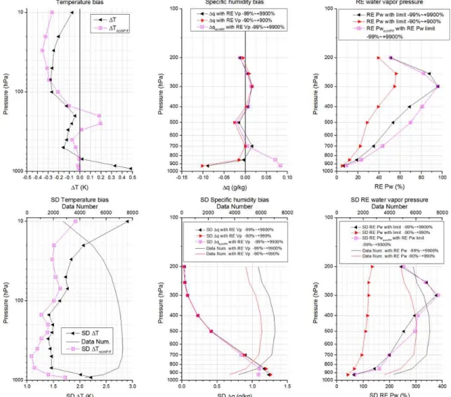
Fig. 2.Comparison of mean temperature bias, mean specific humidity bias, relative error of water vapor pressure, and their SDs. The purple curves show the results of the background ecmPrf, curves without symbols show the number of data points.
3 Comparison results
3.1 Bias and relative error distribution
A total of 7299 profiles matched globally from 2007 to 2010, including 93 511 radiosonde temperature data points and 79 403 dew-point depression data points. On average, a single profile included about 13 layers with temperature data points and 11 layers with humidity data points.
The left graphs in Fig. 2 show the mean temperature bias at each layer and their SDs. The mean temperature bias were all within±0.5 K in each layer. The global mean
tempera-ture bias of 925–10 hPa was−0.09 K, with the SD of 1.72 K.
The wetPrf temperature was a bit higher than the radiosonde temperature in the layers below 700 hPa (pressure larger than 700 hPa), and a bit lower in the layers above 700 hPa. The SD in the layers from 700 hPa to 150 hPa was within the range of 1.4–1.5 K; the SD increased in the higher layers above
100 hPa, with values of 2.07 K in the layer at 20 hPa, increas-ing rapidly to 2.90 K in the layer at 10 hPa. A large SD was also seen in the layers below 700 hPa, with a value of 2.21 K in the layer at 925 hPa.
Fig. 3.Mean water vapor pressure profile of radiosonde, wetPrf, and the background ecmPrf.
difference), in the layers of 925–200 hPa, 74 data points out of the total of 49 772 overstepped the limit, 74 profiles out of the total of 7299 were removed, leaving 7225 profiles. Set-ting the limit of the relative error of water vapor pressure at
−90 % to +900 % (one order of magnitude difference), 1394
data points overstepped the limit, 6202 profiles remained, and 1097 profiles were removed. The comparison of specific humidity and water vapor pressure used the same samples. Although the data filtration slightly influenced the result of temperature comparison and refractivity comparison, it was not suitable to use the same filtration in these comparisons. Because, the temperature comparison and refractivity com-parison were performed in the layers from 925 hPa to 10 hPa, and there were too many data points which overstepped the limit in the layers above 200 hPa.
The middle graphs in Fig. 2 show the mean absolute devi-ation of specific humidity and their SDs. The global mean specific humidity bias at 925–200 hPa was −0.012 g kg−1
(−0.006 g kg−1)with the relative error limit of water vapor pressure−90 % to +900 % (−99 % to +9900 %), and the SD
was 0.666 g kg−1(0.662 g kg−1). The wetPrf specific humid-ity was smaller than radiosonde in near-ground layers, but the background specific humidity was larger. The wetPrf specific humidity was larger than the radiosonde specific humidity around the layer of 300 hPa. The right graphs in Fig. 2 show the mean relative error of water vapor pressure and their SDs. With the limit of −90 % to +900 % (−99 % to +9900 %), the mean relative error in the layers of 925–200 hPa was +33.3 % (+54.6 %), and the SD was 107.5 % (266.0 %), re-spectively. The layers around 300 hPa were more sensitive to the changes in relative error limit. Despite the large mean relative error, the mean absolute deviation was small.
The large mean relative error has relations with the distri-bution of the relative error and the function used to calculate the relative error. The negative relative error can only reach
−100 %, but the positive relative error could be much larger
Fig. 4.Probability density of the relative error of water vapor pres-sure in the layers of 925 to 200 hPa.
than +100 %. Figure 4 shows the probability density of the relative error of water vapor pressure in the layers of 925– 200 hPa without data filtration. Although the peak is located on the negative side, the large positive relative error is greater than the negative error, and the mean relative error is positive. As shown in the figure, the limit of−90 % to +900 % is
rep-resentative.
Figure 5 shows the distribution of the relative error of wa-ter vapor pressure in the layers of 925–200 hPa without data filtration. Similar to the results shown in Fig. 4, the peak is located on the negative side, but the large positive relative error is greater than the negative error. The relative error is much larger if the water vapor pressure value is lower, es-pecially when the radiosonde water vapor pressure value is lower than 0.1 hPa. Taking into consideration the data points for which the radiosonde water vapor pressure is larger than 0.01 hPa/0.1 hPa, the mean relative error of water vapor pres-sure in the layers of 925–200 hPa is +26.9 %/+12.4 %, with a relative error limit of−99 % to +9900 %, while the mean
relative error of water vapor pressure without any radiosonde water vapor pressure limit is +54.6 %.
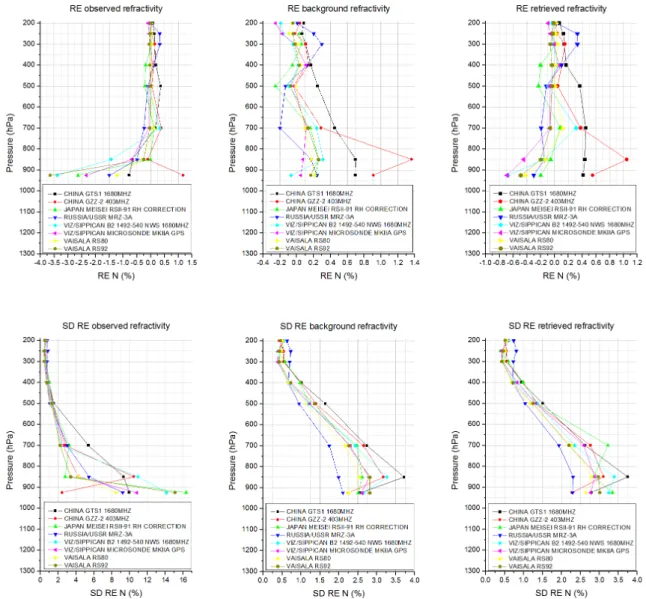
Despite of the the large relative error of water vapor pressure, the refractivity did not change markedly. Figure 6 shows the relative error of the refractivity from radio occulta-tion observaocculta-tion (observed refractivity), the 1DVAR product wetPrf (retrieved refractivity), the background ecmPrf and the refractivity calculated from radiosonde, respectively. The large relative error of water vapor pressure had little effect on refractivity bias. The relative error of refractivity was within
Fig. 5.Distribution of the relative error of water vapor pressure in the layers of 925 to 200 hPa.
Fig. 6.Relative error and SD between the refractivity from the ra-dio occultation observation, retrieval product wetPrf, background ecmPrf and the refractivity calculated from radiosonde data, respec-tively.
3.2 Distribution of extreme relative error of water vapor pressure
In this section, all 7299 profiles were used. Figure 7 shows the distribution of extreme relative error of water vapor pres-sure. The total number of matched water vapor data points in the layers of 925–200 hPa is 49 698, of which four and 626 had a positive relative error larger than +9900 % and +900 %, respectively. The peak was located in the layer at 300 hPa. There are mainly three types of cases. In the first case, the value of radiosonde water vapor pressure was extremely low in this layer but normal in the layers nearby. Usually, this low radiosonde water vapor pressure occurred in a single layer, so there would be a large positive relative error in this layer but normal in the layers nearby. The radiosonde water vapor pressure on the layer below could be 1000 % higher than the value in these layers, and the value in the layer above could
Fig. 7.Distribution of extreme relative error of water vapor pres-sure. The black curve shows the probability of data whose relative error of water vapor pressure is larger than +900 %, the red curve shows the probability of data whose relative error of water vapor pressure is smaller than−90 %. The green curve shows the proba-bility of case 1 described in the paper.
aEquations (7)–(9) were used. The water vapor pressure relative error limit was−90 % to 900 %.bThe first number was a profile number of temperature comparison and
the second number was a profile number of humidity comparison.
500 hPa. The number of the third case was small compared to the second case.
In all, 70 out of the total 49 698 data points in the layers of 925–200 hPa had a negative relative error larger than−99 %
and 768 were larger than−90 %. The peak was located at
200 hPa, due to the systematic humidity bias in layers above 200 hPa. The number of extreme negative relative errors was much smaller compared with the extreme positive ones in the layers below 300 hPa. Most of extreme negative relative er-ror in lower layers belonged to this case, in which the value of wetPrf water vapor pressure was extremely low in the layer but normal in lower and higher layers. The extremely low water vapor pressure seemed to be inconsistent with the real atmosphere (e.g., in the profile of C003.2008.287.11.55, the water vapor pressure was 1×10⁻⁶hPa at the height of
5.7–6.3 km), and the quality control process did not elimi-nate these data points. A single profile could have more than one layer of the extremely low water vapor pressure. About 7.6 % of the wetPrf profiles included at least one layer of ex-tremely low water vapor pressure, the mean total thickness of the extremely low water vapor pressure layer in a single profile was about 414 m. The majority of this phenomenon occurred in layers below 10 km, especially in the altitude re-gion of 2–8 km, but it also occurred in layers above 10 km. Figure 8 shows the distribution of the probability of the pro-file which included extremely low water vapor pressure (less than 2×10⁻⁶hPa). Most of the extremely low water vapor
pressure occurred below 10 km and were located in the lat-itude region of−45 to 45◦, especially in subtropical zone,
and most of the extremely low water vapor pressure occurred above 10 km and were located in the latitude region of−90
to−45◦ and 45 to 90◦. This phenomenon was often
con-comitant with smaller observed refractivity, smaller retrieved refractivity and higher retrieved temperature than those of background. If the observed refractivity was much smaller than background, the 1DVAR process trended to generate lower water vapor pressure and higher temperature. If the
refractivity bias was large enough, the retrieved water vapor pressure might be extremely low or even negative. But things were different in near-ground layers, statistics indicated that the extremely low water vapor pressure phenomenon could be concomitant with larger observed and retrieved refractiv-ity than background when altitude was less than 1 km, and lower temperature than background when altitude was less than 2 km. Overall, the large value regions in Fig. 8 indicated that large negative refractivity bias in COSMIC observation and background ECMWF analysis occurred frequently in those regions.
We have developed an 1DVAR retrieval algorithm which generated temperature and specific humidity profiles using COSMIC’s refractivity profile and ECMWF analysis. Tem-perature profile and humidity profile were retrieved from the observed refractivity profile, and the background was ecm-Prf data. Our 1DVAR process also generated the extremely low water vapor pressure data points. The results showed that the error covariance matrixes had significantly influenced on the retrieval profiles. The extremely low water vapor pressure could be abated if the the error covariance matrixes were ad-justed properly. However, this would make the retrieved wa-ter vapor pressure profile closer to the background, and the temperature profile was also affected.
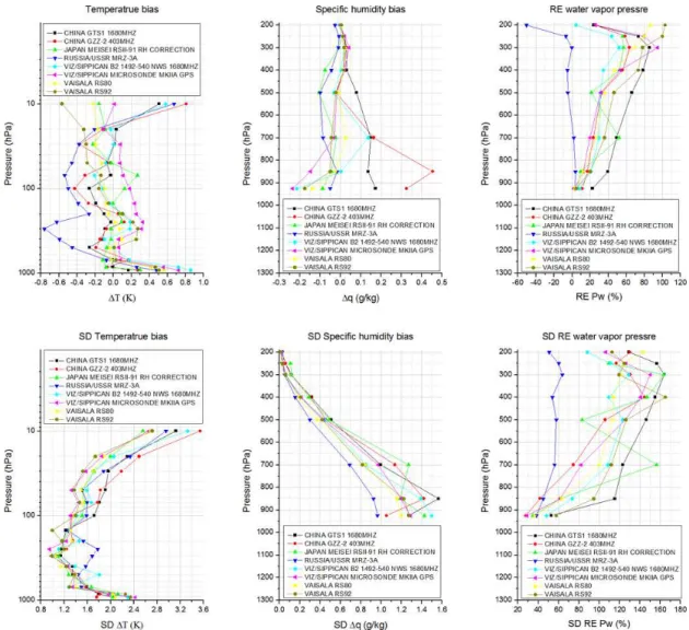
3.3 Comparison of the results with different radiosonde types
Fig. 8.Distribution of the probability of the profiles which contains extremely small humidity data (Pw<2×10⁻⁶hPa). The grid is 5◦×5◦.
two types of VIZ (USA), and VAISALA RS80 and RS92. However, there was a problem in that the wetPrf product is produced through an 1DVAR retrieval process using the ECMWF analysis as the background, and it is therefore af-fected by the different background errors in different regions. Therefore, the comparison is more likely to indicate how the wetPrf data match those from certain types of radiosonde in certain regions. In this comparison, the radiosonde data were set as the benchmarks. It was assumed that the error of a certain kind of radiosonde type would remain the same in different regions. The method used was the same as that in the comparisons described above (Eqs. 7–9). An inverse pro-cess is needed to determine the differences among different radiosonde types. For example, a lower curve in mean tem-perature bias figure indicates that the radiosonde type will yield higher temperature data compared with the other types. The comparison results are shown in Fig. 9 and the mean bias results are shown in Table 2. The left graphs in Fig. 9 show the results of temperature comparison. Most of these radiosonde types showed similar performance. However, MRZ-3A was unique, in that it had much higher tempera-ture compared with the other radiosonde types, especially at layers around 300 hPa. Conversely, VIZ/SIPPICAN MI-CROSONDE MKIIA GPS had lower temperature than oth-ers. The results indicated that the temperatures of the two ra-diosonde types used in China were slightly higher than those of the other radiosonde types. GTS1 showed better perfor-mance than GZZ-2, and GZZ-2 had larger SD at higher lay-ers than the other types if the error of COSMIC product re-mained the same in different regions.
The middle graphs in Fig. 9 show the absolute devia-tion of specific humidity in layers from 925 hPa to 200 hPa. MRZ-3A and JAPAN MEISEI RSII-91RH CORRECTION
had larger value in layers above 700 hPa compared to the other types. In the layers below 850 hPa, VIZ/SIPPICAN MI-CROSONDE MKIIA GPS had the largest positive bias, but in other layers its bias was small. The two radiosonde types used in China had much smaller specific humidity in layers below 500 hPa. The graphs on the right in Fig. 9 show the rel-ative error of water vapor pressure in layers from 925 hPa to 200 hPa. MRZ-3A was still unique, it had negative mean rel-ative error while the others had positive mean relrel-ative error. GZZ-2 showed similar performance to the others. However, GTS1 still had much lower water vapor pressure values than the others, and its SD was the largest.
3.4 Influence of background data
Fig. 9.Differences in mean temperature bias, mean specific humidity bias, relative error of water vapor pressure and their SDs between COSMIC and different radiosonde types. Radiosonde data is the benchmark.
than that in the other regions. As shown in the figure, the re-trieved refractivity was much more similar to the background than to the observation, and so were the SDs. The error of wetPrf data was affected by the background error, and the background error showed considerable differences between different regions. The figure of the relative error of refrac-tivity is similar to the figure of the specific humidity bias in Sect. 3.3.
Although some studies have indicated that COSMIC is suitable as a benchmark (Sun et al., 2010; He et al., 2009; Ho et al., 2010), we feel that the retrieval product could be used as benchmark if no better method is available, or if the precision requirement is not particularly strict, or if the back-ground error is well known. As the refractivity observation is not affected by background, the observed refractivity profile is more suitable to be used as a benchmark than the 1DVAR retrieval product. There were noticeable differences between different versions of the wetPrf data, and improvement of the retrieval process may reduce the bias.
4 Conclusions
Fig. 10.Relative error and SD between the refractivity of different radiosonde types and the refractivity from the 1DVAR product wetPrf, radio occultation observation, and background, respectively.
of about 0.666 g kg−1. The mean absolute deviation of spe-cific humidity was small, but the relative error was signif-icantly large. The mean relative error of water vapor pres-sure in the prespres-sure range of 925–200 hPa was about +33 % to +55 %, depending on the different data filtration used in this paper. The peak of positive relative error was located at about 300 hPa. The large relative error might have been due to the extremely small humidity data of radiosonde or wet-Prf, or to the differences in the rate of decrease in humid-ity. The quality control process of COSMIC failed to detect these abnormal extremely small humidity data. The majority of this phenomenon occurred in subtropical zone. The ex-tremely small humidity data were generated by 1DVAR pro-cess when the observed refractivity was significantly smaller than background. The large relative error of water vapor pres-sure had little effect on refractivity. The 1DVAR retrieval process would reduce the refractivity bias and the standard
deviation in near-ground layers. The differences between retrieved refractivity and observation were small on layers above 200 hPa.
was funded by the National Natural Science Foundation of China (41075011) and Special Fund for Meteorology Research in the Public Interest (GYHY201006037).
Edited by: J.-P. Pommereau
References
Christy, J. R. and Norris, W. B.: Discontinuity issues with radiosonde and satellite temperatures in the Australian re-gion 1979–2006, J. Atmos. Ocean. Tech., 26, 508–522, doi:10.1175/2008JTECHA1126.1, 2009.
Fu, E.-J., Zhang, K.-F., Ka-yea, M., Xu, X.-H., John, M., Anthony, R., Gary, W., and Yuriy, K.: Assessing COSMIC GPS radio oc-cultation derived atmospheric parameters using Australian ra-diosonde network data, Procedia Earth and Planetary Science, 1, 1054–1059, 2009.
Goff, J. A.: Saturation pressure of water on the new Kelvin scale, T. Am. Soc., Heating Air-Cond. Eng., 63, 347–354, 1957. Hajj, G. A., Lee, L. C., Pi, X., Romans, L. J., Schreiner, W. S.,
Straus, P. R., and Wang, C.: COSMIC GPS ionospheric sensing and space weather, Terr. Atmos. Ocean. Sci., 11, 235–272, 2000. Hajj, G. A., Ao, C. O., Iijima, B. A., Kuang, D., Kursinski, E. R., Mannucci, A. J., Meehan, T. K., Romans, L. J., de la Torre Juarez, M., and Yunck, T. P: CHAMP and SAC-C atmospheric results and intercomparisons, J. Geophys. Res., 109, D06109, doi:10.1029/2003JD003909, 2004.
He, W., Ho, S.-P., Chen, H., Zhou, X., Hunt, D., and Kuo, Y.-H.: Assessment of radiosonde temperature measurements in the upper troposphere and lower stratosphere using COS-MIC radio occultation data, Geophys. Res. Lett., 36, L17807, doi:10.1029/2009GL038712, 2009.
Ho, S.-P., Zhou, X., Kuo, Y.-H., Hunt, D., and Wang, J.-H.: Global evaluation of radiosonde water vapor wystematic biases using GPS radio occultation from COSMIC and ECMWF analysis, Re-mote Sens., 2, 1320–1330, doi:10.3390/rs2051320, 2010. Kishore, P., Namboothiri, S. P., Jiang, J. H., Sivakumar,
V., and Igarashi, K.: Global temperature estimates in the troposphere and stratosphere: a validation study of COSMIC/FORMOSAT-3 measurements, Atmos. Chem. Phys., 9, 897–908, doi:10.5194/acp-9-897-2009, 2009.
Kuo, Y.-H., Wee, T.-K., Sokolovskiy, S., Rocken, C., Schreiner, W., Hunt, D., and Anthes, R. A.: Inversion and error estimation of GPS radio occultation data, J. Meteorol. Soc. Jpn., 82, 507–531, doi:10.2151/jmsj.2004.507, 2004.
Miloshevich, L. M., V¨omel, H., Whiteman, D. N., Lesht, B. M., Schmidlin, F. J., and Russo, F.: Absolute accuracy of water vapor measurements from six operational radiosonde types launched during AWEX-G and implications for AIRS validation, J. Geo-phys. Res., 111, D09S10, doi:10.1029/2005JD006083, 2006. Rocken, C., Anthes, R., Exner, M., Hunt, D., Sokolovskiy, S., Ware,
R., Gorbunov, M., Schreiner, W., Feng, D., Herman, B., Kuo, Y.-H., and Zou, X.: Analysis and validation of GPS/MET data in the neutral atmosphere, J. Geophys. Res., 102, 29849–29866, 1997. Seidel, D. J., Sun, B., Pettey, M., and Reale, A.: Global ra-diosonde balloon drift statistics, J. Geophys. Res., 116, D07102, doi:10.1029/2010JD014891, 2011.
Steiner, A. K., Kirchengast, G., and Ladreiter, H. P.: Inversion, er-ror analysis, and validation of GPS/MET occultation data, Ann. Geophys., 17, 122–138, doi:10.1007/s00585-999-0122-5, 1999. Soden, B. J. and Lanzante, J. R.: An assessment of
satel-lite and radiosonde climatologies of upper tropospheric water vapor, J. Climate, 9, 1235–1250, doi:10.1175/1520-0442(1996)009¡1235:AAOSAR¿2.0.CO;2, 1996.
Sun, B., Reale, A., Seidel, D. J., and Hunt, D. C.: Comparing radiosonde and COSMIC atmospheric profile data to quantify differences among radiosonde types and the effects of imper-fect collocation on comparison statistics, J. Geophys. Res., 115, D23104, doi:10.1029/2010JD014457, 2010.
Wang, J. and Zhang, L.: Systematic errors in global ra-diosonde precipitable water data from comparisons with ground-based GPS measurements, J. Climate, 21, 2218–2238, doi:10.1175/2007JCLI1944.1, 2008.
Wang, J., Carlson, D. J., Parsons, D. B., Hock, T. F., Laurit-sen, D., Cole, H. L., Beierle, K., and Chamberlain, E.: Per-formance of operational radiosonde humidity sensors in di-rect comparison with a chilled mirror dew-point hygrometer and its climate implication, Geophys. Res. Lett., 30, 1860, doi:10.1029/2003GL016985, 2003.
Ware, R., Exner, M., Feng, D., Gorbunov, M., Hardy, K., Herman, B., Kuo, Y., Meehan, T., Melbourne, W., Rocken, C., Schreiner, W., Sokolovskiy, S., Solheim, F., Zou, X., Anthes, R., Businger, S., and Trenberth, K.: GPS sounding of the atmosphere from Low Earth Orbit: Preliminary results, B. Am. Meteorol. Soc., 77, 19– 40, doi:10.1175/1520-0477(1996)077¡0019:GSOTAF¿2.0.CO;2, 1996.