Department of Chemical Engineering, University of Novi Sad, Novi Sad, Serbia PharmEng Technology Inc., Toronto, Ontario, Canada
SCIENTIFIC PAPER
UDK 517.912:515.143.2:511.14
DOI: 10.2298/HEMIND0805269C
METHOD FOR DESIGN OF FEEDBACK
CONTROL SYSTEMS
New concept of algebraic characteristic equation decomposition method is presented to simplify the design of closed-loop systems for practical applications. The method consists of two decompositions. The first one, decomposition of the characteristic equa-tion into two lower order equaequa-tions, was performed in order to simplify the analysis and design of closed loop systems. The second is the decomposition of Laplace va-riable, s,into two variables, damping coefficient, ζ, and natural frequency,ωn. Those two decompositions reduce the design of any order feedback systems to setting of two complex dominant poles in the desired position. In the paper, we derived explicit equa-tions for six cases: first, second and third order system with P and PI. We got the ana-lytical solutions for the case of fourth and fifth order characteristic equations with the P and PI controller; one may obtain a complete analytical solution of controller gain as a function of the desired damping coefficient. The complete derivation is given for the third order equation with P and PI controller. We can extend the number of spe-cified poles to the highest order of the characteristic equation working in a similar way, so we can specify the position of each pole. The concept is similar to the root locus but root locus is implicit, which makes it more complicated and this is simpler explicit root locus. Standard procedures, root locus and Bode diagrams or Nichol Charts, are neither algebraic nor explicit. We basically change controller parameters and observe the change of some function until we get the desired specifications. The derived me-thod has three important advantage over the standard procedures. It is general, alg-ebraic and explicit. Those are the best poles design results possible; it is not possible to get better controller design results.
It has been stated many times that the chemical process control theory is inadequate, resulting in poor connection with application. The good theory must be useful not only to process control engineers for design, but should be also developed to accommodate the need and skills of the potential users in application. You can-not expect users to understand complicated theories, so the best control theory should be as simple as possible.
Laplace transform simplifies the linear differential equations into algebraic polynomial equations in the La-place transform variable, s. Algebraization is very im-portant simplification which we use for controller de-sign. A root locus curve is a plot of the roots of the closed-loop characteristic equation as a function of the controller gain. As the gain rise the root locus for third order system changes so that two critical roots move to-ward the limit of stability of critical axe and one non- -critical move in less critical region. We design the P controller by choosing P so that the relative stability of the closed-loop system to have a damping coefficient of about 0.3.
The procedure includes graphing polynomial roots, drawing lines of constant damping coefficient and cros-sing this two lines and estimating the value of P con-troller. This procedure is not simple, it is iterative and it
Correspondence: A. M. Cingara, 172 Kennard Ave., North York, Onta-rio, Canada, M3H 4M7.
E-mail: [email protected] Paper received: February 28, 2008. Paper accepted: June 30, 2008.
is not analytic. This is the standard procedure used in many various new textboxes [1–9].
In this paper, we will develop a simpler concept to get the explicit values of P and PI controller that will locate the closed loop poles in the proper position with the required damping coefficient (relative stability) va-lue in one step without graphing the root locus.
In our paper, the new obtained results are more complicated then the root locus analysis, but analytical results may be obtained for the higher order transfer functions (n = 3, 4, 5).
THE METHOD DEVELOPMENT
Roffel and Rijnsdorp [10] used the polynomial de-composition method for the calculations of frequency stability limits with the domain decomposition for the value of ζ = 0. They divided the system closed loop characteristic equation with the value (s2 +ωu2) to get the
stability limits. Their detailed calculation is presented in the case of third order system with P controller. But for the controller design we need relative stability, not the stability limits.
To solve the problem of relative stability, Mitrović [11] proposed a change of variable s of the form
2 1 ζ
ζω −
− = n
s , into the characteristic equation, and
obtained complex equation with two variables, ζand ωn.
Mitrović's method is different and much more com-plicated then method of Roffel and Rijnsdorp. In this paper, we will show how to improve the quantitative possibilities of the standard methods of complex vari-ables combining the two above methods.
On the first polynomial decomposition level, we will decompose high order polynomial into two lower level polynomials as Roffel and Rijnsdorp [10] did. The second level of decomposition is the domain decom-position. The Laplace complex domain, s, is decom-posedinto two real subdomains ζ and ωn, like Mitrovic
[11] did. The double decomposition results in decom-position of the closed loop characteristic equation into three equations in real domains (ζ,ωn). During
decom-positions, the complex number calculations are not used. The obtained equations are in such a form that all standard mathematical methods for the real function of real variable can be used without any problems. The physical meaning is the usual. The complex equations and complex domain completely disappear.
It is easier to solve many lower order equations than a few higher order one. Hence, using decomposi-tion, one may analytically solve more problems. For ex-ample, it is possible to set more poles into the desired positions, without solving high order polynomials. This analytical method is global in the sense that it is easier to analyze the effect of changes of all parameters in-cluded. Consequently, the method can be used to com-pare control loops with different transfer functions and closed loop structures. This kind of analysis is not pos-sible to conduct with classical local design structure.
The method provides a clear picture of absolute sta-bility and response speed and some picture of relative stability. Both parameters in the PI controller provide limits of parameter values and one may estimate the ef-fect of parameter design on process response.
One can argue that analytical methods cannot be competed with today’s high computational power avail-able to engineers. But analytical methods are the engi-neering way to understand and solve problems and to control the computer calculations, and one must also strengthen the leading role of engineer instead of search-ing for algorithms [13]. The point is that we need both; human and computer power, and those powers are not comparable, they are interactive and compatible.
The new derived method has three important ad-vantages over the standard procedures: It is general,
algebraic and explicit, which is significant advantage over the standard methods. Standard methods are not general, not algebraic and not explicit.
When designing the P controller with standard spe-cific frequency or root locus method, we have to draw different graph for every single specific case, so the me-thods requires to repeat the calculation procedure for every particular design. The results presented in this pa-per are better:
1. general means that we have derived general algebraic formulas for all first, second and third order system with P and PI controller. Using those formulas we can solve all first, second and third order problems;
2. algebraic and explicit means that if we insert the specific data for the process and closed loop specifi-cation we get the controller design explicitly in one step.
The equation derived in this paper solved the case of first, second and third order process with P and PI controller explicitly for every possible case. I derived the equations up to the 5th order. There is no reason that higher order equation cannot be solved manually or by computer program. All the equations have a clear phy-sical meaning and all the parameters of the characte-ristic equations are connected analytically with funda-mental parameters ζ and ωn. We will now apply new
method systematically on first, second and third order system. In the case of third order system with P con-troller, we will compare the Roffel and Rijnsdorp me-thod with the new one.
THE APPLICATION OF THE NEW METHOD FOR THE ANALYSIS AND SYNTHESIS OF FIRST ORDER PROCESS AND P CONTROLLER
Consider the given first order open-loop transfer function:
0 1
1 ) (
a s a s g
+
= (1)
The closed-loop characteristic equation with P controller is:
0 0 1s+a +K=
a (2)
where K is the controller gain. If we specify the closed loop pole position with (a1cs + a0c), where index 1c means specified closed loop parameters, then we can find the appropriate K by dividing the closed loop characteristic equation with the specified closed loop polynomial:
c 1
1 c 0 c 1 0
1 ):( )
(
a a a s a K a s
a + + + = (3)
[–a1s – a0c c 1
1 a
a
]
c 1
1 c 0 0
a a a K
a + − (4)
In order to make that the above denominator divide evenly into the numerator, the remainder (4) must be zero and:
0 c 1
1 c
0 a
a a a
So here is the result, if we want position the closed loop pole into the desired position, K has to have the value given by Eq. (4a).
THE APPLICATION OF THE NEW METHOD FOR THE ANALYSIS OF FIRST ORDER PROCESS AND PI CONTROLLER
Consider the given first order open-loop transfer function (1).
The closed-loop characteristic equation with PI controller is divided with the specified second order term:
1 2 2
I 0
2
1 ( ) ]:( 2 )
[ s s a
T K s K a s
a + + + + ζωn +ωn = (5)
] 2
[ 2
1 1
2
1s a ns a n
a − ζω − ω
−
2 1 I 1
0 2 )
( n a n
T K s a K
a + − ζω + − ω (6)
To make remainder (6) equal zero two equations must be satisfied:
0 1
2a a
K= ζωn− (7)
and
2 1
0 1 1
2
n n a
a a T
ω ζω −
= (8)
And these are the values of controller K and TI that will move the two poles from the given open loop va-lues to the specified complex vava-lues.
THE APPLICATION OF THE NEW METHOD FOR THE ANALYSIS AND SYNTHESIS OF SECOND ORDER PROCESS AND P
CONTROLLER
Consider the second order open-loop transfer func-tion:
0 1 2 2
1 )
(
a s a s a s g
+ +
= (9)
The closed-loop characteristic equation with P con-troller is:
0 0 1 2
2s +as+a +K=
a (10)
where K is the controller gain.
If we want to design the system with a desired closed-loop damping coefficient ofζand ωn, where ωn
is the undamped natural frequency, then it is proposed that Eq. (9) is divided by polynomial:
2 2
2 ns n
s + ζω +ω (11)
The result is:
2 2 2
0 1 2
2 ):( 2 )
(a s +as+a +K s + ζωns+ωn =a (12)
] 2
[ 2
2 2
2
2s a ns a n
a − ζω − ω
−
2 2 0
2
1 2 )
(a − aζωn s+a +K−aωn
In order to make that the above denominator divide evenly into the numerator, the remainder (last row) must be zero and two Equations, (13) and (14), must be sa-tisfied:
0 2 2
1− a n=
a ζω (13)
0
2 2
0+K−a n =
a ζω (14)
Solving Eqs. (9)–(13) and (10)–(14) results in:
0 1
2 a
a K= n −
ζ ω
(15)
The problem is solved forever for all possible pro-cess parameters and closed-loop specifications ζand ωn.
We can also analyze how the result varies with para-meters.
THE APPLICATION OF THE NEW METHOD FOR THE ANALYSIS OF SECOND ORDER PROCESS AND PI CONTROLLER
Consider the second order open-loop transfer func-tion given by Eq. (9).
The closed-loop characteristic equation with PI controller is divided with the specified second order term:
) 2 ( 2
) 2 (
) 2
( : ] ) ( [
3 2
2 3 1 3
2 2 3
2
I 0
2 1 3 3
n n
n n
n n
a a
a a s a a s a
s s
T K s K a s a s a
ζω ζω
ω ζω
ω ζω
− −
− − + −
+ =
= + +
+ + + +
(16)
To make remainder equal zero two equations must be satisfied:
0 2
1 2
2 2 (a 2a ) a
a
K= ωn+ ζωn − ζωn − (17)
and
) 2 (
) 2 ( 2
2 1
2
0 2
1 2
2 I
a a
a a
a a
T
n n
n n
n
ζω ω
ζω ζω
ω
−
− −
+
= (18)
And these are the values of controller K and TI that will move the two poles from the given open loop va-lues to the specified complex vava-lues.
THE APPLICATION OF THE NEW METHOD FOR THE ANALYSIS AND SYNTHESIS OF THIRD ORDER PROCESS AND P CONTROLLER
0 1 2 2 3 3 1 ) ( a s a s a s a s g + + + = (19)
The closed-loop characteristic equation with P con-troller is: 0 0 1 2 2 3
3s +a s +as+a +K=
a (20)
One can obtain the parameters for the limits of sta-bility dividing Eq. (19) by the expression( 2)
u 2+ω
s , as
Roffel and Rijnsdorp [10] did, whereωuis the ultimate
frequency. The quotient is (a3s + a2) and the remainder
is(( ) 2)
u 2 u 0 2 u 3
1 aω s a K a ω
a − + + − , where Ku is the
ulti-mate gain. One wants the denominator to divide evenly into the numerator, so that the remainder equals to zero and one gets two equations with a solutions:
0 3 1 2 u 3 1 2
u , a
a a a K a
a = −
=
ω (21)
If Relation (21) is satisfied then the polynomial of Eq. (20) can be decomposed into the product of two lower order polynomials:
0 ) )(
( 0 u
1 3 2 u 1 2 u
2+ + a +K =
a a s a s ω ω (22)
The first term gives the desired position of system poles, at the limit of stability, and the second term gives the position of the third pole. At the same time, the third order characteristic equation is solved analytically by decomposition.
Analyzing both methods one get the idea to com-bine the method of decomposition with the method of Mitrović in the following way.
If one wants to design the system with a desired closed-loop damping coefficient ofζ, it is proposed that Eq. (20) is divided by polynomial Eq. (23):
2
2 2
n ns
s + ζω +ω (23)
The result is:
n n
ns as a a
s K a s a s a s
a3 3 2 2 1 0 ):( 2 2ζω ω2) 3 2 2 3ζω
( + + + + + + = + − (24)
a3s3 + 2a3ζωns2+a3ωn2s
K a s a a s a
a2−2 3 n)2+( 1− 3 n2) + 0+
( ζω ω
) 2 ( )) 2 ( 2 ( ) 2 ( )) 2 ( 2 ) 2 ( 3 2 2 0 3 2 2 3 1 3 2 2 3 2 2 3 2 n n n n n n n n n n a a K a s a a s a a a a s a a s s a a ζω ω ζω ζω ω ζω ω ζω ζω ζω − − + + − − − − + − + −
In order to make that the above denominator divide evenly into the numerator, the remainder (last row) must be zero and the Eqs. (25) and (26) must be satisfied:
) 2 (
2 2 3
2 3
1 a n n a a n
a − ω = ζω − ζω (25)
) 2 ( 2 3 2
0 n a a n
a
K= +ω − ζω (26)
So, Eq. (20) is decomposed into:
0 ) )(
2
( 2 2 3 0 2 =
+ + + + n n
ns as a K
s
ω ω
ζω (27)
Absolute stability is obtained forζ = 0in Eqs. (25) and (27), and the result is the same as in Eq. (21). Using Eqs (25) and (26) for the design is easy. For the desired value ofζthe analytical solution of natural frequency is:
1 4 ) 4 ( 2 1 2 2 1 2 3 − − + = ζ ζ ζ
ωn a a a a (28)
and the desired analytical solution of controlled gain as function of desired and process parameters is:
3 3 2 2
0 a n 2a n
a
K=− + ω − ζω (29)
For the given damping factor ζ,using Eq. (28) one can calculate the appropriate undamped natural fre-quency ωn. Substituting this frequency into Eq. (29) one
obtains the desired result; the proportional controller gain that gives the desired damping factor in the closed--loop. The quotient provides the position of third pole.
The two Equations, (28) and (29) are the general algebraic and explicit solution to the problem of third order system and proportional controller. The problem is solved forever for all possible process parameters and closed loop specifications, ζ. We can also check how the result varies when we vary parameters.
Example 1
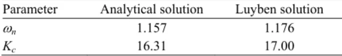
Consider the process of three isothermal reactors [14] with P controller. The parameters of the system are
a0 = a3 = 1 and a1 = a2 = 3, and the Luyben's controller gain is K = Kc/8, where Kc is the gain of the Luyben's controller. The result of application the Eqs. (28) and (29) is shown in Table 1.
Table 1. Comparison of new analytical and Luyben's results forζ = 0.316 and P controller
Parameter Analytical solution Luyben solution
ωn 1.157 1.176
Kc 16.31 17.00
The error is minimal and the results are practically identical.
Towill [15] gives the extensive explanation how the third-order model can be efficiently used for the ap-proximation of higher order model including the models with dead time. For the higher order (4 and 5) model the functional dependences became highly complicated, and the use of these models is restricted to individual cases.
THE APPLICATION OF THE NEW METHOD FOR THE ANALYSIS OF THIRD ORDER PROCESS AND PI CONTROLLER
) 2 ( 2 )
2 (
2
) (
3 2 2
3 1 3
2
2 3 2
2
1 0
2 1 3 2 4 3
n n
n n
n n
a a a
a s a a
s a s
s
T K s K a s a s a s a
ζω ζω
ω ζω
ω ζω
− −
− + −
+
+ = +
+
+ + + + +
(30)
To make remainder equal zero two equations must be satisfied:
0 3
2 3
1 3 2 2
)) 2 ( 2 2
( 2
) 2 (
a a
a a
a a a K
n n
n n
n n
− −
− −
+
+ −
=
ζω ζω
ζω ζω
ζω ω
(31)
and
The obtained equations are exactly what one need: the parameters solution of standard control problem as function of all given process parameters and desired closed-loop dominant poles. It is important to notice that this result for PI control is obtained easier than the result for P control. To get result for P control, it is ne-cessary to solve the first equation, for the PI control this solutions is not necessary.
The performance criterion is simple: for the given damping factor of dominant poles find the biggest K and consequently biggest ωn before system becomes
un-stable or not appropriate for some other reason. For the values of damping factor equal to zero one obtain two equations for ultimate values Ku and TIu.
For higher order PI processes, surprisingly, the so-lution can be also obtained analytically. The only pro-blem is that the functions became more complicated. Again, there is no limit of system order (5) that can be efficiently used in the practice, except the number of terms in the two functions. This paper will now analyze another example.
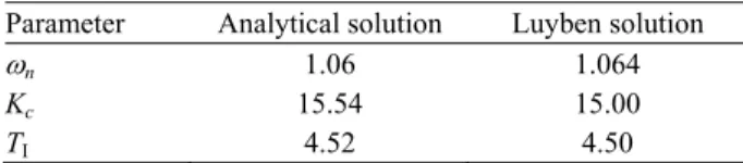
Example 2
Consider the same example of three isothermal re-actors as before Luyben [14], but now with PI con-troller. The parameters of this system models are a0 = = a3 = 1 and a1 = a2 = 3, and the controller gain K = = Kc/8.
Using Eqs. (31) and (32) for PI controller, we obtain the solutions for the desired damping coefficient. The results are compared with the Luyben's one in Tab-le 2. The results for Kc and TI are obtained for the value
ωnfrom Luyben's example.
Table 2. Comparison of new analytical and Luyben's result for
ζ= 0.316 for PI control design
Parameter Analytical solution Luyben solution
ωn 1.06 1.064
Kc 15.54 15.00
TI 4.52 4.50
The results are practically the same, the method is working properly and it is general, algebraic and explicit.
CONCLUSION
The proposed general method gives the analytical global solution for the design of the high order linear feedback control. This means, that not only the solution for one specified transfer function is obtained, but the solutions for all possible combinations of parameters of transfer function of the specified shape. For the P
con-troller one gets the solution as two equations, which can be solved completely analytically for the open-loop trans-fer function of third, fourth and fifth order. For the PI
controller the solution can be expressed analytically for any order, and the highest order is limited by the prac-tical possibility of analyprac-tical derivation of long division. The method gives a clear picture of absolute stabi-lity, response speed, and some measure of relative sta-bility. The role of both parameters in PI controller, and the new limit of stability for TI parameter is given. The simple method is derived for calculation the values of controller parameter in order to obtain the desired posi-tion of damping factor and the natural frequency. The simple explanation is given for the ultimate value of na-tural frequency and the method of calculation of this va-lue and the desired vava-lue is derived. The results are ex-pressed as real functions of real parameters.
The results presented in this paper are: general, which means that we have derived the general algebraic formulas for all possible first, second and third order system with P and PI controllers. To solve any first, se-cond and third order problem you can use the derived algebraic formulas, insert your data for your process and controller specifications and design the controller using one explicit calculation.
Notations
P − Proportional PI − Proportional-integral
ai − Parameters of open-loop transfer functions (i = 0,n) K− Controller gain
Kc− Controller gain in Luyben's example
g(s) − Transfer function p− Pole
s – Laplace transform variable z− Zero
TI− Controller integral time constant
ζ− Damping factor
ωn− Undamped natural frequency
ωnu− Ultimate natural frequency ))
2 ( 2 (
)) 2 ( 2 (
2 )
2 (
3 2
2 3 1 2
0 3 2
2 3 1 2
2 3 2
2 I
a a
a a
a a a
a a a
a a
T
n n
n n
n n
n n
n n n
ζω ζω
ω ω
ζω ζω
ω ζω
ω ζω ω
− −
−
− −
− − +
−
Subscripts
u − Ultimate n − Natural
LITERATURE
[1] K. J. Astrom, R.M. Murray, Feedback Systems, An In-troduction for Scientists and Engineers, Princeton Uni-versity Press, 2008.
[2] O. Bosgra, H. Kwakernaak, G. Meinsma, Design Methods for Control Systems, Notes for Duch Instutute of Systems and Control, 2008.
[3] H. Jack, Dynamic System Modeling and Control, Clay-more University, 2007 (http://clayClay-more.engineer.gvsu.edu) [4] B. Roffel, B. Betlem, Process Dynamics and Control:
Modeling for Control and Prediction, Willey Blackwell, 2006.
[5] S. Christian, Course of Multidisciplinary and Controlled Systems, Ruhr, Universitat Bochum, 2005 (http:// //www.atp.ruhr-uni-bochum.de).
[6] D. Seborg, T. Edgar, D. Mellichamp, Process Dynamics and Control, 2nd Ed., Wiley, 2004.
[7] W. Bequette, Process Control Modeling, Design and Simulation, Prentice Hall Int., 2003.
[8] P. Chau, Process Control: A First Course with Matlab, Cambridge Series in Chemical Engineering, 2002. [9] T. Marlin, Process Control: Designing Processes and
Control Systems for Dynamic Performance, Mc Graw Hill, New York, 1995.
[10] B. Roffel, J.E. Rijnsdorp, Process Dynamics, Control and Protection, Ann. Arbor Sci. Pub., 1982, p. 62. [11] D. Mitrović, Graphical Analysis and Synthesis of
Feed-back Control Systems: Part I, Theory and Analysis; Part II, Synthesis; Trans. AIEE, Part III, January, 1959. [12] G. J.Thaler, R. G.Brown, Analysis and Design of
Feed-back Control Systems, McGraw-Hill, New York, 1960, Ch. 10.
[13] Z. J. Palmor, R. Shinar, Design of Advanced Process Controllers, AIChE. J. 27 (1982) 793.
[14] W. L. Luyben, Process Modeling, Simulation and Con-trol for Chemical Engineers, McGraw-Hill, New York, 1990, pp. 363, 481.
[15] D. R. Towill, Coefficient Plane Models for Control Sys-tem Analysis and Design, Research Studies Press, John Wiley, Chichester, 1981.
IZVOD
NOVI JEDNOSTAVAN ALGEBARSKI METOD GEOMETRIJSKOG MESTA KORENA ZA
PROJEKTOVANJE SISTEMA AUTOMATSKOG UPRAVLJANJA
Tehnološki fakultet, Univerzitet u Novom Sadu, Novi Sad, Srbija PharmEng Technology Inc.,Toronto, Ontario, Canada
Naučni rad
Prikazan je metod algebarske dekompozicije karakteristične jednačine da bi se uprostilo projektovanje zatvorenog kola za praktične primene. Metod se sastoji od dve dekompozicije. Prva dekompozicija je deljenje karakte-ristične jednačine na dve jednačine nižeg reda da bi se uprostilo projekto-vanje regulatora. Druga dekompozicija je zamena s-promenljive koja ima nejasan fizički smisao sa dve variable koje imaju potpuno jasan fizički smisao a to su faktor prigusenja, ζ, i prirodna frekvenca, ωn.Ove
dekom-pozicije uprošćavaju projektovanje sistema na pozicioniranje kompleksnih dominantnih polova u željene pozicije. U radu su izvedene sve jednačine za sisteme prvog, drugog i trećeg reda sa P i PI regulatorima, ukupno šest analitičkih jednačina. Slične jednačine mogu se izvesti analitički do jedna-čina petog reda, a pomoću kompjuterskih programa verovatno do n-tog reda.U slučaju sistema trećeg, četvrtog i petog reda karakteristične jedna-čine sa P i PI regulatorima mogu se dobiti kompletna analitička rešenja regulatora K kao funkcije željenog faktora prigušenja. Izvedeni metod ima tri važne prednosti u odnosu na standardne postupke. On je generalan, al-gebarski i eksplicitan, što nijedan standardni postupak nije. Ovi su rezultati matematički najbolji mogući.
Key words: Algebraic • Control Sys-tems • Root Locus Analysis and Syn-thesis • Controller design