An Analytical Model for Hydraulic Fracturing
in Shallow Bedrock Formations
by Jos´e S´ergio dos Santos
1, Thomas Paul Ballestero
2, and Ernesto da Silva Pitombeira
3Abstract
A theoretical method is proposed to estimate post-fracturing fracture size and transmissivity, and as a test of the methodology, data collected from two wells were used for verification. This method can be employed before hydrofracturing in order to obtain estimates of the potential hydraulic benefits of hydraulic fracturing. Five different pumping test analysis methods were used to evaluate the well hydraulic data. The most effective methods were the Papadopulos-Cooper model (1967), which includes wellbore storage effects, and the Gringarten-Ramey model (1974), known as the single horizontal fracture model. The hydraulic parameters resulting from fitting these models to the field data revealed that as a result of hydraulic fracturing, the transmissivity increased more than 46 times in one well and increased 285 times in the other well. The model developed by dos Santos (2008), which considers horizontal radial fracture propagation from the hydraulically fractured well, was used to estimate potential fracture geometry after hydrofracturing. For the two studied wells, their fractures could have propagated to distances of almost 175 m or more and developed maximum apertures of about 2.20 mm and hydraulic apertures close to 0.30 mm. Fracturing at this site appears to have expanded and propagated existing fractures and not created new fractures. Hydraulic apertures calculated from pumping test analyses closely matched the results obtained from the hydraulic fracturing model. As a result of this model, post-fracturing geometry and resulting post-fracturing well yield can be estimated before the actual hydrofracturing.
Introduction
Fractured bedrock aquifers are an important source of drinking water and nowadays some worldwide com-munities are completely dependent upon them. In some cases, where these communities are small and at the same time located far from surface water supplies, it is much less expensive to explore and develop the bedrock
1Departamento de Construc¸˜ao Civil, Instituto Federal de
Educac¸˜ao Ciˆencia e Tecnologia do Cear´a, Av. Treze de Maio, 2081, CEP: 60040-531, Fortaleza, CE, Brazil; [email protected]
2Corresponding author: Department of Civil Engineering,
University of New Hampshire, 238 Gregg Hall, UNH, Durham, NH 03824; [email protected]
3Departamento de Engenharia Hidr´aulica e Ambiental,
Universidade Federal do Cear´a, Campus do Pici, Bloco 713, CEP 60451-970, Fortaleza, CE, Brazil; [email protected]
Received October 2009, accepted May 2010. Copyright2010 The Author(s)
Journal compilation2010 National Ground Water Association. doi: 10.1111/j.1745-6584.2010.00727.x
groundwater rather than to construct surface water infrastructure (reservoirs, treatment plants, transmission mains, etc.).
With these numbers in mind, one wonders if it is possible to estimate the predictable alteration in bedrock structure in order to enhance the hydraulic efficiency and thereby well yield. For more than 50 years, the petroleum industry has used hydraulic fracturing as a mean to increase the productivity of gas and oil reservoirs. This technique is also used in the United States to produce increased yields of water wells. Nevertheless, there are significant differences between hydraulic fracturing of deep sedimentary formations and shallow bedrock.
The main objective of this paper is to propose a practical methodology to predict the consequences of hydraulic fracturing unproductive wells, especially a method that can be employed before hydrofracturing in order to obtain the estimates of the potential hydraulic benefits of hydraulic fracturing. As a test of the method-ology developed in this paper, data collected by Stewart (1974) in two pumping wells were used for verification.
Theoretical Background
Flow in Fractured Aquifers
Flow in fractured aquifers is strongly dependent on fracture geometry, water availability, and fracture interconnectedness. This means that the greater our understanding about the nature of rock fractures, the greater our ability to analyze the hydraulic processes that occur in this kind of formation. Unfortunately, due to its highly complex nature and our limited ability to “see” into the formations, fractured bedrock characteristics cannot everywhere be deterministically characterized. Although some information is obtained from borehole logs, drilling cores, outcrops, and/or geophysical surveys, the resolution and spatial continuity of this data are not sufficient to completely describe the fracture system. As a result, either deterministic methods that apply numerous simplifying assumptions or stochastic characterization methods are commonly applied to fracture geometry in order to make presenting results possible in terms of the most likely system behavior (Renshaw 1996).
Over the past several decades, research is nearly uni-form in identifying that flow in fractured rocks is depen-dent of the degree of interconnection among fractures which in turn is dependent on fracture density, orienta-tion, length, and aperture (Long and Witherspoon 1985). A highly fractured and interconnected bedrock system tends to behave as a porous medium and, consequently it exhibits higher permeability than otherwise. Systems which have a high standard deviation in their fracture orientations tend to display larger hydraulic conductivity than systems with parallel fractures (Pitombeira 1994). The fracture length plays an important role in determin-ing the system permeability because it is more probable that long fractures intersect other fractures than do shorter fractures. Lastly, hydraulic or effective aperture is consid-ered one of the most important factors affecting flow in fissured reservoirs. Theoretical and experimental research has demonstrated that the flow in a fractured media is proportional to the fracture aperture cubed (Witherspoon
et al. 1980). This means that small changes in aperture can produce great changes in the fracture transmissivity.
The relationship between flow and fracture aperture is known as the “cubic law” and was obtained by applying the Navier-Stores equations and Darcy’s law to a parallel plate system. Since it uses Darcy’s law in its derivation, the flow must be laminar. In comparison to a porous medium in which the Reynolds number below 10 implies laminar flow (Todd 1959), for a relatively smooth fracture surface the transition from laminar to turbulent flow is at a Reynolds number of about 2400 (Witherspoon et al. 1980). However, research has found that as the fracture roughness factor increases, the critical Reynolds number was significantly less than 2400. Geertsma and de Klerk (1969) suggested a practical critical Reynolds number for fracture flow equal to 750, and Meyer Associates Inc. (2004) suggests 1000.
For laminar flow between two parallel plates, the volumetric flowQ [L3 T−1] for a single fracture width normal to the flow direction is given by:
Q= −b3 ρg
12µ∇h (1)
whereb [L] is the hydraulic aperture;µ [M L−1 T−1] is the fluid dynamic viscosity;ρ[M L−3] is the fluid density; ∇h is the hydraulic gradient in the flow direction; andg
[L T−2] is the acceleration of gravity.
Considering Equation 1 as Darcy’s law applied to a fractured medium, fracture transmissivity, Tf [L2 T−1], is:
Tf =b3
ρg
12µ (2)
Hydraulic aperture,b[L], relates to average mechan-ical aperture,w[L], by:
b3= w 3
f (3)
where the factor “f” is:
f =1+8.8ε
b 1.5
when(ε/b) >0.033, (4)
and
f =1 when(ε/b)≤0.033. (4a)
wheref is the wall fracture roughness correction factor andε[L] is the absolute roughness of the fracture surface.
ε/b represents the relative roughness of the fracture wall compared with the size of the flow field.
Aquifer Testing
rock systems. Streltsova (1988) states that analysis of the pressure behavior of a naturally fractured formation during flow tests presents a challenge because this behavior is diverse in character and is generally represented by multislope response curves to which conventional methods are not applicable.
Kruseman and de Ridder (1990) agree by stating that conventional well-flow equations, developed primarily for homogeneous aquifers, do not adequately describe the flow in fractured rock systems. However, they also state that some exceptions can be found in hard rock of very low permeability if fractures are numerous enough and are evenly distributed throughout the rock. In this case, the fluid only flows through the fractures and the formation becomes hydraulically similar to that of an unconsolidated, homogeneous porous media aquifer.
In any event, when analyzing pumping test data it should be understood that the well drawdown represents the sum-total effect of the hydraulic characteristics of the aquifer within the cone of depression, including all irregularities (Uhl and Sharma 1978).
With historic hydraulic data in hand of pre and posthydraulic fracturing for two wells, the first step in this study was to perform pumping test analyses utilizing five different analytical methods in an attempt to iden-tify which method better described the aquifer hydraulic behavior (drawdown data), especially before hydraulic fracturing. The methods that were used included: Theis (1935), Cooper and Jacob (1946), Hantush and Jacob (1955), Papadopulos and Cooper (1967), and Gringarten and Ramey (1974). Theis’ method was used with the intention of verifying how far the data were from that of an ideal solution as well as to use as the basis for post-fracture comparisons. The semilog graph for Jacob’s method was extremely useful in determining the type of deviation the formations displayed compared with an ide-alized aquifer. For example, patterns such as confined, unconfined, leaky, wellbore storage, recharge, or imper-meable boundaries. In addition, Jacob’s method helped to identify (relatively) the degree of interconnection existing among fractures.
Mechanics of Hydraulic Fracturing
Basic Concepts
Great oil and gas reservoirs have been found within consolidated sedimentary formations, such as sandstones, limestone, dolomites, and shale. But despite the fact that a sedimentary rock matrix can store enormous amounts of fluid, it may have low permeability. If such a formation contains a fracture set, the system can be conceived as a double porosity system, for which a continuous approach can be applied. In this case, the rock matrix is said to have great storage capacity and low permeability (primary porosity) and the fracture system represents near-infinite permeability, yet, low storage (secondary porosity).
When a new oil or gas well is drilled and it displays a very low production rate of a magnitude that it is not economically feasible, it is normally considered to be
eligible for hydraulic fracturing. Basically, a hydraulic fracturing operation consists of pumping a fluid at a high pressure into a selected section of unlined borehole. Smith and Shlyapobersky (2000) explain what happens when the fracturing fluid penetrates into the formation: “If fluid is pumped into a well faster than the fluid can escape into the formation, inevitably pressure rises, and at some point something breaks. Because rock is generally weaker than steel, therefore what breaks is usually the formation, resulting in the wellbore splitting along its axis as a result of tensile hoop stresses generated by the internal pressure.” When the pump is shut down, pressure inside the created fracture dissipates and the confining stresses tend to lead the fracture walls to return to their initial position (the fracture closes). To avoid this, a propping agent (proppant) such as sand or bauxite is commonly blended into the fracturing fluid in order to prop open the fracture when fluid pressure is reduced.
Fracture Geometry
Existing rock fracture systems are complex and result from historic and present day stresses. What is presented here is a simplified view of how fractures can propagate within the constraints of present day existing stress fields. Normal stresses in a formation will ultimately determine fracture geometry (Geertsma and de Klerk 1969). Similar to a chain that breaks at its weakest link, a fracture opens in the direction of the least principal stress. The magnitude and direction of the principal normal stresses in bedrock are basically a function of depth, and if the ground is horizontal, the principal normal stress directions are vertical and horizontal.
The estimation of vertical stress is straightforward. Goodman (1989) states that it is safe to assume that the vertical normal stress is equal to the weight of the overlying rock (Equation 5), which is approximately 0.027 MPa/m. In comparison to the vertical stress, hori-zontal stresses are a bit more complicated to determine. Goodman (1989) quotes an investigation made by Brown and Hoek (1978) over a number of published values of in situ stresses in which they found a hyperbolic relation between the ratio of average horizontal (σh,ave) and the average vertical stresses (σv,ave)and the depth (Z). This simple but meaningful relation is given in Equation 6.
σv,ave=ρgZ (5)
0.30+100 Z <
σh,ave σv,ave
<0.50+1500
Z (6)
An analysis of Equation 6 reveals that for depths less than 142 m (466 feet), horizontal stresses are expected to be always greater than vertical stress. The opposite happens with depths greater than 3000 m (9800 feet). This means that fracturing shallow formations generates horizontal fractures; whereas fracturing deep formations generates vertical fractures.
in shallow formations, and many of them were explored to estimate their form in the subsurface. According to Murdoch and Slack (2002), in several dozen cases the vicinity of the fracture was excavated to provide detailed cross sections. As a result, they found that nearly circular fractures had grown to several meters or more in the horizontal dimension.
This information is very important when applied to water wells. Geological studies have shown that fractured rock aquifer permeability generally decreases with depth. In igneous rock, this happens because weathering and tectonic effects that cause the appearance of natural fractures diminish with depth. As a consequence, the well depth for a water supply well in crystalline bedrock is generally about 100 m (328 feet) or less. In the Brazilian state of Cear´a, the average well depth in this kind of formation is 63.4 m (208 feet) (CPRM 2007), and 103 m (340 feet) in New Hampshire (Wunsch et al. 2004). Therefore, fracturing wells in these formations and at these depths is expected to produce horizontal fractures.
Hydraulic fracturing lies at the interface of fluid mechanics and rock mechanics (Brady et al. 1992). Sev-eral idealizations have been proposed to model fracture propagation within rock formations. These models have used concepts from the theory of elasticity, linear elastic fracture mechanics, Newtonian and non-Newtonian fluid mechanics, and even thermodynamics. dos Santos (2008) proposed a very practical method for predicting the aper-ture and extent of hydraulically induced fracaper-tures.
Model Description
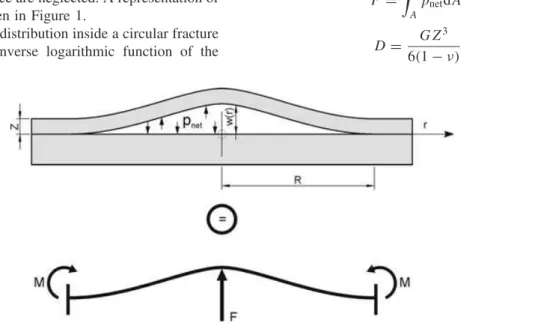
In this model, fracture propagation inside the forma-tion was treated by means of an analogy to a deformable circular plate with fixed edges. Net pressure at the supe-rior fracture surface acts as a vertical load, from bottom to top, and therefore the effect of increasing the fracture fluid pressure is the uplift of the superior stratus. Strains in the inferior fracture surface are neglected. A representation of this model can be seen in Figure 1.
The net pressure distribution inside a circular fracture is governed by an inverse logarithmic function of the
radius (Geertsma and de Klerk 1969). This means that great pressure is found in proximity to the well but it falls rapidly when moving away from the well and toward the fracture tip, and it is zero at the tip. It is this characteristic which allows the substitution of the pressure distribution by a concentrated load applied at the fracture center (dos Santos 2008, p. 114, 115).
In order to obtain an analytical solution and at the same time keep the problem mathematically tractable, the following assumptions were made: (1) the formation is an elastic, infinite, impermeable, homogeneous, and isotropic medium, characterized by its shear modulus, Poisson’s coefficient, and fracture toughness; (2) an incompressible, Newtonian fluid is injected in fracture center at a constant flow rate; (3) flow is everywhere laminar; (4) net pressure at the fracture tip is zero; (5) the fracture propagates under mobile equilibrium condition, which implies that the mode I stress intensity factor equals the fracture toughness during propagation; and (6) in order to calculate the strains (fracture aperture) the logarithmic load generated by the net pressure is represented by an equivalent concentrated load applied in the fracture center (Figure 1).
Analysis
The uplift of the vertical stratus above the fracture plane is assumed to be equal to the fracture aperture,
w(r)[L]. Therefore, the fracture form is determined by the elastic surface, which is given by Love (1927, p. 475):
w(r)= F 16π D
R2−r2−2r2lnR
r
(7)
where R [L] is the fracture radius, F [ML T−2] is the concentrated load (force) applied in the fracture center, andD [M L2 T−2] is the bending rigidity of the plate, defined by:
F =
A
pnetdA (8)
D= GZ
3
6(1−ν) (9)
where pnet [M L−1 T−2] is the net pressure inside the fracture,Z [L] is the stratus thickness above fracture,G
[M L−1 T−2] is the rock shear modulus, and ν is the Poisson’s coefficient.
The maximum strain,ww [L], is found in the fracture
center and it is equal to:
ww= F R2
16π D (10)
Therefore, Equation 7 can be rewritten as:
w(r)=ww
1−r R
2
+2r
R 2
lnr
R
(11)
dos Santos (2008) determined the fracture volumeV
[L3] as:
V =
A
w(r)rdrdθ ⇒ (12)
V =wwπ R 2
4 (13)
Average aperture,wave[L], is obtained from Equation 13:
wave= ww
4 (14)
For a circular fracture in an infinite medium and subjected to a concentrated loadF applied at its center, the mode I stress intensity factor,KI [M L−1/2 T−2], can be written as (Paris and Sih 1965, p. B15 to B16):
KI= F
(π R)3/2 (15)
The net pressure distribution in a circular fracture can be written as (Geertsma 1989, p. 87):
pnet(r)= 6Qiµff
π w3 ave
lnR
r (16)
where Qi [L3 T−1] is the injecting fluid flow rate and µff[M L−1T−1] is the fracturing fluid dynamic viscosity. The magnitude of the equivalent load can be determined throughout the preceding equation for a certain time, t, greater than zero as follows (dos Santos 2008, p. 120 to 121):
F =
A
pnet(r)dA⇒ (17)
F =
192Qiµff π w3
w
π R2= 192QiµffR 2
w3 w
(18)
Propagation Regimes
A propagation regime is defined as the regime in which one particular process overcomes all the other in terms in energy and mass balance (Lhomme 2005, p. 44 to 75). For the fractured rock, two regimes can be identified: (1) toughness-dominated regime and
(2) viscosity-dominated regime. In the first, energy dissi-pation due to viscous flow inside the fracture is negligible when compared with the necessary dissipation required to break the rock bonds at the crack tip. In the latter regime occurs the opposite.
To identify the governing regime of the propagation process, the use of the nondimensional temporal param-eter, τ, is made. τ quantifies the relative importance of dissipated energy to extend the fracture inside the rock in relation to dissipated energy from fluid flow inside the fracture. Determination ofτ is made through the following equations (Lhomme 2005, p. 54):
τ = K
′18t2 µ′5
ffE′13Q 3 i
1/2
(19)
K′=4
2
π 1/2
KIC (20)
µ′=12µ (21)
E′= 2G
(1−ν) (22)
If τ ≪1, the regime is viscous-dominated. Conversely, if τ ≫1 fracture propagates under toughness-dominated regime (Lhomme 2005, p. 58).
In order to identify which regime dominates the prop-agation process, the model calculates, using Equation 19, the pumping time that corresponds toτ =1. Subsequently the model verifies how much this time represents of the total pumping time. If it is less than 50%, the model selects the toughness-dominated regime equations and solves the problem. If it is the contrary, the chosen equations are the viscous-dominated regime (dos Santos 2008, p. 122).
Analysis becomes time-dependent by the introduction of the mass balance between the injection flow and the fracture volume V. This approach neglects the dynamic effects during propagation. Therefore for a hydrofracturing pumping time, t:
V =Qit (23)
After the identification of the propagation regime by Equation 19, Equations 10, 13, and 15 are solved as function of time in Equation 23 in the case of toughness-dominated propagation regime. In the case of viscous-dominated propagation regime, Equations 10, 13 and 18 are solved as function of time in Equation 23. As a result,
R and ww are obtained. These values are applied in Equation 16 in order to calculate the net pressure during the hydrofracturing operation. As a result, for a radial, no-fluid-loss propagation, dos Santos (2008) proposed the following explicit relations and regimes:
Toughness-dominated regime (τ ≫1):
ww=
324Q7iKIC4 (1−ν)4 π5Z12G4
1/11
R=
1024Q2 iG2Z6 9π3K2
IC(1−ν)2
1/11
t2/11 (25)
pnet=
384Qiµff π w3
w ln
R
rw
(26)
Viscosity-dominated regime (τ ≪1):
ww=
1152Q3iµff(1−ν) π3Z3G
1/6
t1/3 (27)
R=
32Q3iZ3G
9π3µ
ff(1−ν)
1/12
t1/3 (28)
pnet=
384Qiµff π w3
w ln
R
rw
(29)
whereKIC[M L−1/2 T−2] is the rock fracture toughness, E′ [M L−1 T−2] is the rock plane strain modulus, rw [L] is the wellbore radius, t [T] is the pumping time for the hydraulic fracturing. These relations were used in this paper for simulating the fracture geometry and propagation pressure.
Methodology
Well Description
Stewart (1974) drilled two wells in the crystalline bedrock at the University of New Hampshire horticultural farm, Durham, New Hampshire. The two wells are 207 m (680 feet) apart, each has a diameter of 152.4 mm (6 inches) and were drilled to different depths; one 146 m (480 feet) and the other 92 m (302 feet). The deeper one (Well A) is in granite and the shallower one (Well B) is in a schistose rock. Following the drilling, the wells were logged and then were pumped at different rates for different periods of time. The longest pumping test was approximately 8 h. Before hydraulic fracturing, the safe yield of Well A was estimated to be 0.91 m3/h (4 gpm) and Well B was 0.82 m3/h (3.6 gpm).
Pumping tests were carried out in three stages: before hydraulic fracturing (1973), immediately after hydraulic fracturing (1973), and 1 year after the treatment (1974). A total of 10 pumping tests were conducted, five in each well. Tests performed before hydraulic fracturing revealed no hydraulic communication between the wells.
Hydraulic Fracturing Description
According to Stewart (1974), one packer was set 27.4 m (90 feet) above the bottom of Well A and another packer was set 15.2m (46.7 feet) above the bottom of the Well B. During fracturing, water was pumped into the well below the packers at a rate of about 0.0227 m3/s (360 gpm). The rock fractured at approximately 13.79 MPa (2000 psi) and the pumping time was about 60 min. In the two wells, a total of 8176 kg of fine Ottawa sand (20/40
mesh) was blended into the water and served as a propping agent. In Well A, a total of 75.04 m3 (19,824 gallons) of this slurry was used to sustain pressure and propagate the fracture. The pressure chart of Well B indicated that fracturing initiated at a pressure of approximately 6.21 MPa (900 psi). But 45 min after the water injection began, the packer loosened and the fracturing pressure was completely lost. A total of 50.88 m3 (13,776 gallons) of slurry were injected in Well B.
Pumping tests were initiated immediately after the fracturing. The safe yield of Well A was 5.68 m3/h (25 gpm), an increase of 4.77 m3/h (21 gpm), or 525%, over prefracturing. Well B was also stimulated, from 0.82 m3/h (3.6 gpm) to 3.41 m3/h (15 gpm), or an increase of 317%. It is important to mention that after hydraulic fracturing the two wells were then in hydraulic communication, as indicated by the water level data during the individual well pumping tests.
Pumping Test Analyses
To assess the effects of hydraulic fracturing for these two wells, the first step consisted of determining the aquifer properties such as transmissivity and storativity. The wells were drilled in an anisotropic medium, so the calculated transmissivity from the numerical methods refers to the average aquifer transmissivity within the cone of depression. Also, since the radius of influence is a function of pumping time and at the same time anisotropy does not allow easy definition of the representative elemental volume, it is expected that these parameters could also be affected by the pumping time. After estimating aquifer transmissivity, Equation 2 was used to calculate hydraulic aperture.
Well A
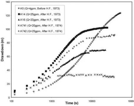
Figures 2 and 3 are semilog plots of drawdown vs. time for Well A and Well B pumping tests, respectively. In an ideal aquifer such as portrayed by the Theis method (1935), well drawdown data should plot as a straight line after the initial period. For Well A, the only pumping test performed before hydraulic fracturing, the plot resembles a straight line, but wellbore storage and leakage effects can also be identified. After fracturing, these effects became more perceptible. For Well A, the Papadopulos method was the method that best fit the observed data. Results are presented in Table 1.
As can be seen in Table 1, hydraulic fracturing sig-nificantly altered the aquifer parameters (transmissivity, hydraulic aperture) in the vicinity of the wellbore. Val-ues of storage coefficient reflect the average valVal-ues found in the region (Pulido 2003). The aging of the well 1 year after fracturing appears to have resulted in increased leak-age, since at both pumping rates, the leakage effects occur at earlier times (Figure 2).
Well B
Figure 2. Pumping test drawdown results for Well A (H.F.: hydraulic fracturing).
Figure 3. Pumping test results for Well B (H.F.: hydraulic fracturing).
boundary or pumping more than the safe yield. This is evident in the late time drawdown values in these tests. The Gringarten-Ramey Method (1974) was the only model that adequately represented this data. It should be noted that the barrier boundary effect at these pumping rates was removed by the hydraulic fracturing. This can be seen by observing drawdown evolution in the later times in tests B25, B743, and B744. The Well B transmissivity, that was originally less than 1.0×10⁻⁷ m2/s, was increased more than 285 times after the hydraulic fracturing. In this well, the hydraulic apertures
calculated for tests B3 and B4 physically associate with an actual observed fracture that was not in the zone that was hydraulically fractured. The hydraulically stimulated wellbore zone had no delineated fractures (no hydraulic aperture) before fracturing, and after fracturing the hydraulic aperture was calculated to be 0.3 mm, as estimated by Equation 2.
Connectivity
Table 1
Well A —Transmissivity and Storativity Calculated by Papadopulos-Cooper Method (1967)
Pumping Test
A5 A14 A16 A741 A742
Hydraulic fracturing
Before After After After After
Transmissivity (m2/s) ×(1E+7)
24.10 242.6 161.7 636.8 172.4
Storage coefficient
8.73E-06 4.56E-7 1.09E-03 3.66E-07 5.56E-04
Hydraulic aperture (mm)
0.16 0.34 0.29 0.46 0.30
fluids to flow through the rock matrix toward the fracture and subsequently be collected at a well. In fractured rocks, this does not happen because of the relative impermeability of the rock matrix. This means that in the case of fractured rock the primary and significant flow occurs in the fracture system. In order to enhance well efficiency in fractured crystalline rock, it is necessary to create changes in the systems’ main hydraulic parameters: aperture and connectivity.
Knudby and Carrera (2006) state that in hydrogeol-ogy, “connectivity” is most often used as a reference to the physical presence of connected zones of either high or low conductivities. In other words, if a system exhibits the existence of a high-conductivity path that exhibits rela-tively higher groundwater flow and allows for early solute arrival, it is said that this system possesses good con-nectivity. However, how to measure it, and under what conditions, and how it affects various types of hydrologic response, is still debated.
Studies on bedrock fracture connectivity have re-vealed that high-transmissivity zones are better connected than low-transmissivity zones and estimates of storativity from Jacob’s method (1946) contain information not only on near-well materials, but also on the degree of hydraulic interconnectedness between the pumping and observation wells. The aquifer transmission property (T )
and storage property (S) can be combined into one single parameter called hydraulic diffusivity (Freeze and Cherry 1979). Although it is a relatively meaningless
parameter for porous media applications, it has become extremely meaningful as a means of quantifying aquifer connectivity.
Despite the lack of quantification, there is evidence that the storage coefficient, S, and therefore also the hydraulic diffusivity, D (D=T /S), as interpreted from Jacob’s method, are related to connectivity, and that this relationship has to do with the presence of connected features (Knudby and Carrera 2006). As heterogeneity causes estimates of storage coefficient obtained from Jacob’s method to be different from their actual values, terms such as apparent storativity, Sa, and apparent diffusivity, Da [L2 T−1], are used to refer to the values obtained from Jacob’s method. Equation 30 defines apparent diffusivity as:
Da= T Sa
(30)
Values of apparent diffusivity were calculated for all 10 tests made in the two UNH wells and they are presented in Table 2.
As expected, hydraulic fracturing significantly in-creased the system’s connectivity as judged by the increase of apparent diffusivity. In the case of Well A, even when removing the anomalous test (A741), the aquifer’s apparent diffusivity was increased more than 20-fold. With respect to Well B, it seems that the new apparent diffusivity is more than one order of magnitude larger than the original.Dafor test B743 is low because the very short duration of the test yielded hydraulic characteristics masked by the wellbore storage effect.
Most Likely Hydraulic Fracturing Response
Experiments performed by Paillet (1994) and Paillet and Olson (1994) demonstrated that fracturing wells drilled in crystalline, naturally fractured bedrock does not create new fractures. Stewart (1974) confirmed this by geophysical characterizations (temperature, caliper, multiple electrode resistivity, natural gamma radiation, induced gamma radiation, and neutron radiation) that were performed before and after hydraulic fracturing in Wells A and B. This phenomenon can be explained by linear elastic fracture mechanics theory. According to this theory, the fracture tip is a stress concentrator (Anderson 1995). When the well section becomes subjected to the high pressure from the pumped injection fluid, the first place
Table 2
Apparent Diffusivities for Wells A and B (from Cooper-Jacob results)
Well Test # Hydraulic Fracturing Da(m2/d) Well Test # Hydraulic Fracturing Da(m2/d)
A A5 Before 35 B B3 Before 80
A A14 After 601 B B4 Before 121
A A16 After 662 B B25 After 1742
A A741 After 74,098 B B743 After 2
Table 3
Parameters from Hydraulic Fracturing Operations
Rock Fluid Fracture
G (GPa) ε(mm) Vi(m3) t (s) Qi(m3/s) µff (Pa-s) η
Well A 32.0 0.3 75.04 3849.32 1.95E-02 1.27E-03 0.98
Well B 42.5 0.3 50.88 2400.00 2.12E-02 1.27E-03 0.97
that exceeds the rock’s tensile yield stress is the fracture tip. So, in this case, stimulation does not create new fractures but it opens and extends the existing fractures.
Results
Geophysical logs of Well A revealed that only the existing water-bearing fracture was sensibly affected by the hydraulic fracturing. This fracture is located approximately 3 m (10 feet) above the wellbore bottom. With respect to Well B, Stewart (1974) writes that the fracture located approximately 35 m (115 feet) below the ground surface was believed to be the principal or only, water-bearing fracture before hydraulic fracturing. In this case, due to its position above the packer, this fracture was not affected by hydraulic fracturing. This means that all hydraulic improvement in this well was obtained through a formerly nonproducing fracture.
In order to predict the fracture geometry that is antic-ipated to result from hydraulic fracturing, the parame-ters found in Table 3 were employed in the equations presented previously. These values were obtained from Stewart (1974), Schultz (2009), Backers (2005), Backers and Stephansson (2007), Staroselsky (1999), Morrow and Lockner (2006), Clark (1966), and others. Here,Vi [L3] is the injected slurry (water+sand +detergent) volume andη is the fracture porosity. Simulation results are pre-sented in Table 4, these results compare very favorably to the hydraulic data of Tables 1 and 5.
Before hydraulic fracturing, the pumping test data demonstrated that Wells A and B were not in hydraulic communication; however, after fracturing they were. According to Stewart’s logs, the stimulated fracture in Well A is located at a depth of 143 m and Well B is
Table 4
Results of Hydraulic Fracturing Simulation (Equations 1, 4, 5, and 6)
Fracture Geometry
Final Hydraulic Aperture
Estimated
Transmis-sivity
R(m) ww(mm) w (mm) bf(mm) Tf(m2/s)
Well A 206 2.25 0.56 0.34 244E-07 Well B 175 2.11 0.53 0.30 181E-07
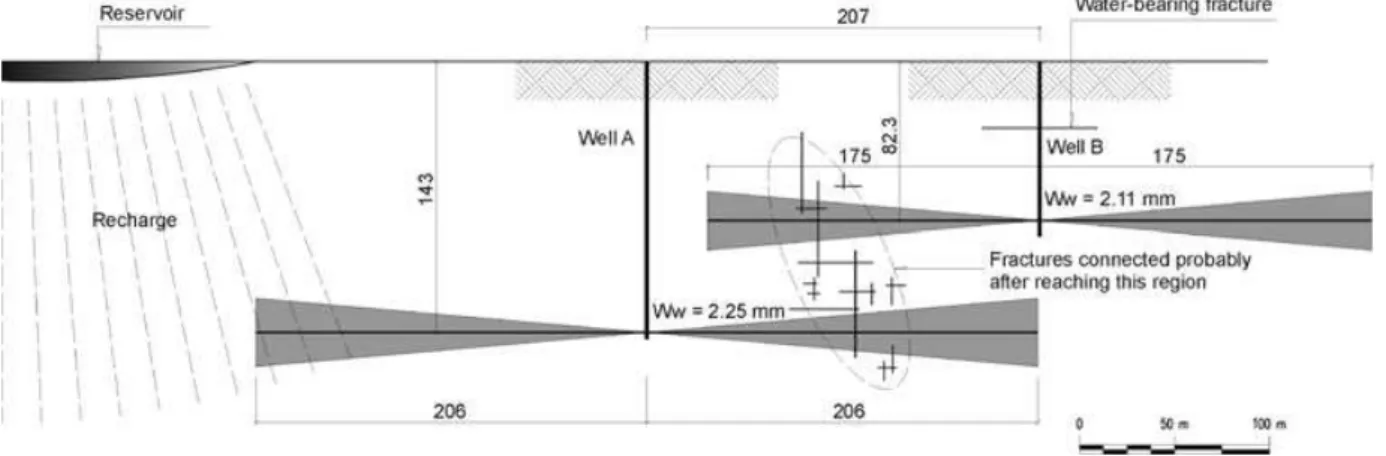
at 82.3 m. As can be visualized in Figure 4, fracture propagation possibly created an overlapping region for the two wells, or they could have both connected to another fracture that linked them together (the wells are 207 m [679 feet] apart). Murdoch and Slack (2002) state that the fracture trace occurs within shaded triangular envelop with mean dip of 10◦, as represented in Figure 4.
The computed maximum aperture values of the two fractures are about 2.20 mm, and their average values are about 0.50 mm. It should be noted that this aperture affords the 20/40 sand to be injected into the formation since its size is between 0.425 and 0.85 mm. Although these fractures seem very thin, they have great flow capacity compared with the preexisting condition. Effects of roughness and porosity on the fracture flow were considered (Table 3), and this led to corrected values of the hydraulic aperture of 0.34 mm for Well A (compared with an average of 0.35 mm from Table 1) and 0.30 mm for Well B (compared with an average of 0.28 mm from Table 5). In the case of Well B, differences found in estimated vs. computed from pumping test data aperture can be justified by possibly the proppant inside the fracture after the fracturing pressure was reduced.
Paillet (1994), Paillet and Olson (1994), Paillet and Ruhl (1994), and Paillet and Hanscom (2000) from studies in more than 20 fractures reported that hydraulic fracturing increased the capacity of individual fractures by a factor of about 10. This result was also found by Schuring (2002) in 27 projects, in which hydraulic conductivity increased from 5 to 153 times, with an average of 34 times. However, Paillet stated that there is no guarantee
Table 5
Well B —Transmissivity and Storativity Calculated by Gringarten and Ramey (1974)
Pumping Test
B3 B4 B25 B743 B744
Hydraulic fracturing
Before Before After After After
Transmissivity (m2/s) ×(1E+7)
0.37 0.93 124.0 67.2 169.50
Storativity 1.41E-04 1.59E-01 3.43E-04 3.63E-01 1.23E-01 Hydraulic
aperture (mm)
Figure 4. Conceptual hydrogeologic model generated by the dos Santos model (2008).
that hydraulic fracturing will always reach such excellent results.
Another important question is related to the pre-fracturing hydraulic conductivity. High-transmissivity fractures will not allow large pressure development during hydraulic fracturing, and in this case, the fracturing fluid will flow away from the treatment zone almost as fast as it is injected into the well. To reduce this effect, a more viscous fracturing fluid can be used, such as a water-based polymeric gel like guar gum.
Sustainable (or temporary) hydraulic aspects may also affect the success of fracturing operations. Although some post-fractured wells could exhibit high specific capacity during a conventional production test, 3 to 5 d after fracturing, they may not sustain it over periods of a year or more. This may have something more to do with the long-term water depletion of the rock, and appears to be especially significant in drier places like California, or similar Mediterranean climate, in which there is a long dry season over which the rock mass water storage is depleted.
Conclusion
Hydraulic fracturing has been proven to be an effec-tive method to enhance the productivity of wells drilled in consolidated formations, especially for crystalline bedrock (Schultz 2009). Although the technique is widely used for water wells, there is little technical information regarding predicting the effects or success of hydraulic fracturing due to the complexity of the problem. Hydraulic fracturing of low permeability, shallow, fractured formations differs significantly from that in deep sedimentary rocks. Here, the fracturing fluid rarely leaks; the fracture geometry is generally horizontal; and more often instead of creating new fractures, existing fractures are stimulated. Results have shown that stimulated fractures can propagate by dozens of meters, breaking through the formations’ imper-meable boundaries, and consequently improving the sys-tem’s connectivity.
Although developed for homogeneous, isotropic aquifers, Papadopulos’ method (1967) can be considered a
very good method to estimate transmissivity and storativ-ity of fractured aquifers particularly during early pumping times. This is especially important when the ultimate use of a well is taken into consideration. Pumping time is gen-erally short for domestic wells, and in New Hampshire such wells represent 98% of the total number of wells contained in the database (Moore et al. 2002). Domes-tic bedrock wells are 40% of all wells in Cear´a (CPRM 2007).
The Gringarten-Ramey method fitted very well to the data from Well B, and it was the only method used that adequately modeled the aquifer’s impermeable barrier. Papadopulos’ method also fit the data well, and could be used to determine the aquifer parameters for these wells. There is no rigid rule when dealing with fractured aquifers. Several methods have to be employed and compared until a satisfactory result is found.
The methodology presented in this paper can be considered simplistic; however, it is proposed as a means of dealing with an otherwise very complex problem. Nevertheless, even when employing the simplifying assumptions here, the results were extremely satisfactory for the modeled data. Recognizing that all sites are different, data from additional sites should be tested with this model in order to understand limitations and the range of applicability.
Acknowledgments
Support for this research was furnished by FUNCAP (Fundac¸˜ao Cearense de Apoio ao Desenvolvimento Científico e Tecnol´ogico); CAPES (Coordenac¸˜ao de Aperfeic¸oamento de Pessoal de Nível Superior); and the University of New Hampshire. This support is grate-fully acknowledged. The critical time and comments of the anonymous reviewers were also very helpful and are acknowledged.
References
Backers, T., and O. Stephansson. 2007. Time dependent frac-ture growth in intact crystalline rock: new laboratory pro-cedures. In ISRM 11th International Congress on Rock Mechanics, Lisboa, Portugal.
Backers, T. 2005. Fracture toughness determination and micromechanics of rock under mode I and mode II loading. Doctoral thesis, University of Potsdam.
Brady, B., J. Elbel, M. Mack, H. Morales, K. Nolte, and B. Poe. 1992. Cracking rock: progress in fracture treatment design.
Oilfield Review 4, no. 4: 4–17, ISSN 0923-1730.
Brown, E.T., and E. Hoek. 1978. Trends in relationships between measured in situ stress and depth.Int J Rock Mech Min Sci
15, no. 4: 211–215.
Clark, S.P. 1966. In Handbook of Physical Constants, ed. S.P. Clark. NY: Geological Society of America. Series: Geological Society of America Memoir, 97.
Cooper, H.H., and C.E. Jacob. 1946. A generalized graphical method for evaluating formation constants and summarizing well field history.American Geophysical Union Transac-tions, 27, 526–534.
CPRM—Servic¸o Geol´ogico do Brasil. Atlas Eletrˆonico dos Recursos Hídricos e Meteorol´ogicos do Cear´a. 2007. http://atlas.srh.ce.gov.br (accessed February 2005). dos Santos, J.S. 2008. Efeitos do Fraturamento Hidr´aulico
em Aquíferos Fissurais (Effects of Hydraulic Fracturing in Fractured Aquifers), Tese de Doutorado (Ph.D. diss.), Universidade Federal do Cear´a, Brazil.
Freeze, R.A., and J.A. Cherry. 1979.Groundwater. New Jersey: Prentice-Hall Inc.
Geertsma, J. 1989. Two-dimensional fracture propagation mod-els.Recent Advances in Hydraulic Fracturing. Monograph Series, 12, SPE, 81–94. Richardson, Texas.
Geertsma, J., and F. de Klerk. 1969. A rapid method of predicting width and extent of hydraulically induced fracture. Journal of Petroleum Technology 21, no. 12: 1571–1581.
Goodman, R.E. 1989.Introduction to Rock Mechanics, 2nd ed., New York: Wiley.
Gringarten, A.C., and H.J. Ramey. 1974. Unsteady state pressure distributions created by a well with a single horizontal fracture, partial penetration or restricted entry.Journal of the Society of Petroleum Engineers14, 413–426.
Hantush, M.S., and C.E. Jacob. 1955. Non-steady radial flow in an infinite leaky aquifer.American Geophysical Union Transactions36, 95–100.
Knudby, C., and J. Carrera. 2006. On the use of apparent hydraulic diffusivity as an indicator of connectivity.Journal of Hydrology329, no. 3–4: 377–389.
Kruseman, G.P., and N.A. de Ridder. 1990.Analysis and Evalu-ation of Pumping Test Data, 2nd ed., Wageningen, Nether-lands: Int. Inst Land Reclamation Improvement/ILRI. Lhomme, T.P.Y. 2005. Initiation of hydraulic fractures in natural
sandstones. Ph.D. Diss., Technische Universiteit Delft, Netherlands.
Long, J.C.S., and P.A. Witherspoon. 1985. The relationship of the degree of interconnection to permeability in fracture networks. Journal of Geophysical Research 90, no. B4: 3087–3098.
Love, A.E.H. 1927.A Treatise on the Mathematical Theory of Elasticity. New York: Dover. 481 p.
Meyer Associates Inc. 2004.User’s Guide—Meyer Fracturing Simulators, 4th ed. 698 p.
Moore, R.B., G.E. Schwarz, S.F. Clark Jr., G.J. Walsh, and J.R. Degnan. 2002. Factors related to well yield in the fractured-bedrock aquifer of New Hampshire. (U.S. Geo-logical Survey professional paper 1660), ISBN 0-607-98453-8.
Morrow, C.A., and D.A. Lockner. 2006. Physical properties of two core samples from Well 34-9RD2 at the Coso Geothermal Field, 2006–1230. California: U.S. Geological Survey Open-File Report.
Murdoch, L.C., and W.W. Slack. 2002. Forms of hydraulic fractures in shallow fine-grained formations. Journal of Geotechnology and Geoenvironmental Engineering 128, no. 6: 479–487.
Paillet, F.L., and H. Hanscom. 2004. Borehole geophysical char-acterization of hydraulic stimulation of fractured bedrock aquifers.Proceedings of the Symposium on the Application of Geophysics to Engineering and Environmental Problems, ed. Powers, M.H., Ibrahim, Colo., Environmental and Engi-neering Geophysical Society, p. 567–576.
Paillet, F.L. 1994. Hydraulic stimulation of fractured aquifers— a human-induced modification to enhance water production and remediation. InAmerican Water Resources Association Symposium.Jackson Hole, Wyoming, p. 913–921. Paillet, F.L., and J.D. Olson. 1994. Analysis of the results of
hydraulic-fracture stimulation of two crystalline bedrock boreholes. Grand Portage, Minnesota: U.S Geological Survey. Water-Resources Investigations Report 94–4044. Paillet, F.L., and J.F. Ruhl. 1994. Using borehole geophysics to
evaluate the effects of hydraulic stimulation of fractured bedrock aquifers. InSociety of Professional Well Log Ana-lysts Annual Logging Symposium, 35th, Tulsa, Oklahoma, Transactions, U1–U11.
Papadopulos, I.S., and H.H. Cooper. 1967. Drawdown in a well of large diameter. Water Resources Research 3, no. 1: 241–244.
Paris, P.C., and G.C. Sih. 1965. Stress analysis of cracks. Amer-ican Society for Testing and Materials (ASTM)—Special Technical Publication.
Pitombeira, E. 1994. Groundwater flow model for fractured media. PhD diss., University of New Hampshire, Durham, New Hampshire.
Pulido, G. 2003. Some contributions to the hydraulic char-acterization of fractured bedrock formations. Ph.D. diss., University of New Hampshire, Durham, New Hampshire. Renshaw, C.E. 1996. Influence of subcritical fracture growth
on the connectivity of fracture networks.Water Resources Research 32, no. 6: 1519–1530.
Schultz, R.A. 2009. Fractures and Bands in Rock: A Field Guide and Journey into Geologic Fracture Mechanics. Unpublished manuscript.
Schuring, J.R. 2002. Fracturing technologies to enhance reme-diation. Technology Evaluation Report (TE-02-02), GRW-TAC E-Series.
Smith, M.B., and J.W. Shlyapobersky. 2000. Basics of hydraulic fracturing. In Reservoir Stimulation, 3rd ed., ed. M.J. Economides and K.G. Nolte. New York: John Wiley. Staroselsky, A. 1999. The express method of determining the
fracture toughness of brittle materials.International Journal of Fracture98, no. 3–4: 17–52.
Stewart, G.W. 1974.Hydraulic Fracturing of Drilled Water Wells in Crystalline Rocks of New Hampshire. New Hampshire Department of Resources and Economic Development. Streltsova, T.D. 1988. Well Testing in Heterogeneous
Forma-tions. New York: Wiley.
Theis, C.V. 1935. The relation between the lowering of the piezometric surface and the rate and duration of discharge of a well using groundwater storage.American Geophysical Union Transactions 16, 519–524.
Todd, D.K. 1959. Groundwater Hydrology. New York: John Wiley.
Uhl, V.W., and G.K. Sharma. 1978. Results of pumping tests in crystalline-rock aquifers. Ground Water 16, no. 3: 192–203.