Trade-off vs pecking order : a life cycle of financing decisions

(1)

Carlos Manuel Alves Domingues

UMinho|20 12 Dezembro de 2012 Trade-of f vs. P ecking order : A life cy

cle of financing decisions

Universidade do Minho

Escola de Economia e Gestão

Trade-off vs. Pecking order:

A life cycle of financing decisions

Carlos Manuel Alv

(2)

Dissertação de Mestrado

Mestrado em Finanças

Trabalho realizado sob a orientação do

Professor Doutor Artur Rodrigues

Carlos Manuel Alves Domingues

Dezembro de 2012

Universidade do Minho

Escola de Economia e Gestão

Trade-off vs. Pecking order:

(3)

ii

Declaração

Nome: Carlos Manuel Alves Domingues

Endereço electrónico: CarlosUnivMail@gmail.com

Número do Bilhete de identidade: 12697410 Título dissertação ☒ /tese ☐

Trade-off vs. Pecking Order: A life cycle of financing decisions

Orientador (es):

Professor Doutor Artur Rodrigues

Ano de conclusão: 2012 Designação do Mestrado ou do Ramo de Conhecimento do Doutoramento:

Mestrado em Finanças

É AUTORIZADA A REPRODUÇÃO INTEGRAL DESTA TESE/TRABALHO APENAS PARA EFEITOS DE INVESTIGAÇÃO, MEDIANTE DECLARAÇÃO ESCRITA DO INTERESSADO, QUE A TAL SE COMPROMETE.

Universidade do Minho, / / Assinatura:

(4)

iii

Agradecimentos

Tão, ou mais importante que qualquer uma das seguintes é, esta página, onde expresso os meus mais sinceros agradecimentos a todos, sem os quais, nenhuma outra teria sido possível. Desde os que me criaram, passando pelos que confiaram e acompanharam, até aos que ensinaram e em especial, a todos os que acreditaram, deixo aqui o que considero, um pequeno tributo, quando comparado com a imensa paciência, compreensão e disponibiliade, com que moldaram quem sou.

Nesta lista de pessoas extraordinárias, incluo a familia, professores e amigos. De entre os professores, realço com particular destaque, o papel determinante do Professor Doutor Artur Rodrigues, meu orientador, que acompanhou todo o processo, disponibilizou material e realizou sugestões que, indiscutívelmente, valorizaram o trabalho. Ainda, o Professor Doutor Gilberto Loureiro, cujo importante contributo ao nível do tratamento de dados, permitu também, ultrapassar alguns obstáculos que surgiram ao longo do desafio, que foi esta dissertação.

(5)

iv

Trade-off vs. Pecking order:

Um ciclo de vida de decisões de financiamento

Resumo

Com o auxilio das teorias do trade-off e do pecking order, esta dissertação procura estudar se, as decisões de financiamento de empresas, durante o periodo de 1996 até 2007, são consistentes com a ideia de um ciclo de vida de decisões de financiamento. A amostra é constituida por 56420 observações, oriundas de 48 países diferentes.

Os resultados mostram que ambas as teorias apresentam limitações, quer de cariz teórico quer empírico. No entanto, de forma geral, a teoria do trade-off domina a teoria do pecking order, especialmente para empresas em crescimento. Por sua vez, embora o desempenho da teoria do pecking order não se destaque em qualquer uma das fases do ciclo de vida organizacional, este tende a melhorar ligeiramente em fases de maturidade. De facto, testes adicionais revelam que o desempenho da teoria do pecking order é mais severamente condicionado por empresas de diferentes tamanhos e com diferentes quantidades de ativos tangíveis.

Conciliando toda a evidencia encontrada, verificamos que a existência de um ciclo de vida de decisões de financiamento não é, de todo, absurda. Empresas em fase de crescimento demonstram seguir um padrão de financiamento distinto do de empresas mais maduras, onde a escolha de capital próprio das primeiras, contrasta fortemente com a escolha de recursos internos e dívida das segundas, como fontes de financiamento.

Palavras-chave: trade-off, pecking order, estrutura de capital, alavancagem, dívida, capital próprio, ciclo de vida, maturidade, crescimento, estagnação

(6)

v

Trade-off vs. Pecking order:

A life cycle of financing decisions

Abstract

Assisted by the trade-off and pecking order theories, this dissertation, attempts to assess whether the financing decisions of firms, during the period from 1996 to 2007, are consistent with a life cycle of financing decisions. The sample comprises 56,420 firm observations from 48 different countries. Results show that both theories have weaknesses, either from theoretical or empirical nature. Nevertheless, in general, the trade-off dominates the pecking order, especially when growth firms are considered. In turn, while the pecking order performance does not stand out in any stage of the organizational life cycle, it tends to improve, slightly, in later stages of maturity. In fact, additional tests indicate that the performance of the pecking order is most severely constrained when firms are proxied by size and tangibility.

Piecing together all the evidence, we find the existence of a life cycle of financing decisions, anything but absurd. Firms in growth stages, exhibit a financing pattern distinct to that of mature firms, where the choice for equity of the first, strongly contrasts with the choice for internal resources and debt of the second, as financing choices.

Keywords: trade-off, pecking order, capital structure, leverage, debt, equity, life cycle, maturity, growth, stagnancy

(7)

vi

Table of Figures

Figure 1- Diagram of the samples. ... 44

Table of Tables

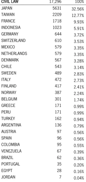
Table 1 - Consitution of the samples by countries (balanced samples)... 45

Table 2 - Consitution of the samples by countries (unbalanced samples) ... 45

Table 3 - Consitution of the samples by industries (balanced and unbalanced samples) ... 46

Table 4 - Consitution of the subsamples by industries (unbalanced samples) ... 47

Table 5 - Summary statistics ... 48

Table 6 - Variables used for the classification in different stages of maturity ... 49

Table 7 - Compound scores and stage attribution ... 49

Table 8 - Trade-off OLS regressions (full balanced and unbalanced samples) ... 50

Table 9 - Trade-off OLS regressions (subsamples) ... 51

Table 10 - Trade-off OLS regressions with control variables (subsamples) ... 52

Table 11 - Leverage OLS regressions ... 53

Table 12 - Correlation between the leverage variables ... 54

Table 13 - Leverage OLS Re, Fe and 2SLS regressions (full unbalanced samples) ... 55

Table 14 - Leverage 2SLS regressions (subsamples) ... 56

Table 15 - Pecking order OLS regressions (full balanced and unbalanced samples) ... 57

Table 16 - Pecking order OLS regression (dissociated deficit) ... 58

Table 17 - Pecking order OLS regression continued (full balanced and unbalanced samples) ... 59

Table 18 - Pecking order OLS regressions (subsamples) ... 60

Table 19 - Pecking order OLS regressions with control variables (subsamples) ... 61

(9)

8

1 - Introduction

Raising funds is a vital operation for any firm. Fortunately, when a firm seeks to raise capital, there is a vast collection of financing instruments at managers’ disposal. Retained earnings may not always be available or enough, but debt and equity, are both feasible alternatives for the same purpose. In the end, the real mystery, boils down to which financing strategies are adopted by firms and why.

Regrettably, many researchers and studies after the puzzle of corporation’s capital structure was first approached half a century ago by Modigliani & Miller (1958), the financial community is still clearly divided about which forces actually drive firms to select one funding source over another. Although many competing theories were developed over the last fifty years, none seems to tell the whole story yet, and some authors even argue that “there is no universal theory of the debt-equity choice, and no reason to expect one. There are several useful conditional theories, however.” Myers (2001, p. 81), “Thus it is probably time to stop running empirical horse races between them as stand-alone stories for capital structure.” Fama & French (2005, p. 580–581).

Despite the lack of consensus, among these theories, two opposing mainstreams appear to dominate the subject of capital structure: trade-off and pecking order theories. While the first prophesies that firms pursuit an optimum capital structure, the second, conceptualizes a hierarchical structure of financing sources. Another underlying cause of their antagonism lays on how both relate several determinants, including investment opportunities and profitability, with leverage. Where the trade-off theory conjectures that leverage is negatively related to growth1 and positively related to profitability2,

the pecking order anticipates an inverse relation3.

Fama and French (2005) believe that “profitability and growth characteristics of firms are central in evaluating their financing decisions.” Curiously, growth and profitability can also be traced back to specific organizational life cycle stages.

1_{The existence of risky debt can induce managers to give up on future positive NPV projects, leading to a suboptimal investment policy (Myers, 1977). For}

this reason, growth firms are expected to use it sparingly.

2_{Debt can be used to shield the taxable income (Modigliani & Miller, 1963) as well as control free cash flows (Jensen, 1986).}

3_{Since growth firms are likely to lack sufficient internal resources to finance their NPV opportunities, debt, will usually be the next best choice. Likewise,}

(10)

9

According to Mueller’s (1972) hypothesis, at early stages, agency problems are nearly nonexistent or negligible since, at this point, managers still own a significant portion of stock and as such, entrepreneurs and stockholders’ interests are conveniently aligned. Additionally, the existence of many investment opportunities that fuel a profit-oriented growth, together with the fact that insufficient internal funds compels firms to resort to external financing, receiving a heightened scrutiny, cements an harmonious relation between managers and stockholders.

Later as firms evolve and competition interferes, managers and stockholders grow apart, to a certain extent, as a result of the ownership dilution that managers undergo, in order to raise capital at previous stages. Furthermore, growth is threatened, and the absence of positive NPV projects, generates a surplus of unused funds, accrued from current activities. Hence, when a firm reaches maturity, dividends4 will often be considered by managers, as the next best alternative to reinvestment.

Eventually, once the initial opportunities fade completely, a stockholder-welfare maximizer manager will either rebuy the outstanding stocks or liquidate the remaining assets and distribute the earnings as a last stream of dividends, to stockholders.

In light of the exposed, could there be a link between the organizational life cycle hypothesis and the capital structure theories? To the best of our knowledge, no relevant past literature explicitly answers this question. Mueller (1972), describes each life stage as a precise set of key characteristics5 that

evolve dynamically during a firm’s existence however, most traditional studies, tend to focus on individual aspects of firms, as if they occurred independently one of another.

We argue that, the failure to acknowledge all the changes that firms endure at each stage, could lead to a dubious assessment of stages and inadequate extrapolations, regarding a firm’s life cycle. Therefore, only with a model that recognizes and incorporates all the relevant changes, simultaneously, are we able to accurately describe each stage of firm development and answer whether a life cycle of financing choices really exists.

4_{Other forms of payout may be considered by managers; i.e., shares repurchase (Grullon & Michaely, 2002).}

5_{Investment opportunities, profitability and dividend policy are some of the most obvious changes that a firm endures as it evolves from younger to more}

(11)

10

To bridge the gap in literature between the organizational life cycle hypothesis and the modern capital structure theories, this study intends to empirically test how the trade-off and pecking order theories perform with samples in different stages of maturity and hopefully, further enlighten our perception about the capital structure of firms.

Resting on a multivariate stage classification system, previously used by Anthony & Ramesh (1992), we find that, on a set of international broad samples, the pecking order theory is consistently outperformed by the trade-off model in every life cycle stage. Additionally, while the trade-off performance degrades when exposed to samples of firms in later stages of maturity, the pecking order displays a slight improvement. Complementary tests also show that the pecking order performance is highly related with other variables like tangibility and size. Altogether, we interpret the evidence as consistent with a life cycle of financing choices, considering that growth and mature firms follow different financing patterns.

The rest of this paper is structured as follows: in the next chapter we present the relevant literature. In chapter 3, we detail the methodology adopted, followed by the data description in section 4. In chapter 5, we examine the results and in section 6 we conclude our findings.

(12)

11

2 - Previous Research

What is the ‘cost of capital’ to a firm in a world in which funds are used to acquire assets whose yields are uncertain; and in which capital can be obtained by many different media, ranging from pure debt instruments, representing money-fixed claims, to pure equity issues, giving holders only the right to a pro-rata share in the uncertain venture? (Modigliani & Miller, 1958, p. 1) With the previous question in mind, Modigliani & Miller (1958), documented the irrelevance theory of capital structure, according to which, firms’ value is not a function of its financial decisions. In other words, backed by the idea that capital markets are perfect, under the deliberately utopic world proposed by Modigliani & Miller (1958), whether a firm decides to finance its assets by issuing pure debt, equity, or any mix of debt-equity, the outcome is the same.

Clearly, the assumptions were too restrictive to mirror a credible reality. However, even though to that extent, the original work could be considered somewhat limited, it rapidly raised the attention of several authors, propelling a series of studies that actively corner stoned the birth of the modern capital theories. Soon, the irrelevance theory became relevant.

2.1 - Trade-off Theory

The static trade-off theory saw light as many of the former assumption were dropped in favor of realism. This time, under the idea that markets are efficient but not perfect, different authors embraced a new reality that acknowledged the existence of taxes, bankruptcy and agency costs. Modigliani & Miller (1963) for one, recognize the positive role of tax shields on leverage while at the same time, alert for the fact that using debt may not always be optimal, due to certain limitations and costs associated with this financial choice. In turn, Jensen & Meckling (1976) and Jensen (1986), discuss potential conflicts of interests between managers and bondholders (shareholders), as a direct result from overusing (neglecting) leverage. While debt can be considered an effective instrument to control financial slack6 or even rebalance the interests of managers and stockholders through repurchase of

6_{A commitment to debt holders, implies the payment of interest with free cash flows that otherwise could be misused at the discretionary will of the}

(13)

12

stock, in excess, can lead to problems of asset substitution7. Also, according to Myers (1977), firms

should issue debt conservatively, as the accumulation of risky debt, could compromise valuable future investment opportunities.

In the current context, the pattern encoded in the trade-off theory becomes evident. Firms ought to track a delicate equilibrium – target capital structure – by carefully weighting the costs8 and benefits9 of

resorting to debt, in view to maximize its value. This constitutes the main precept of the classic, static trade-off theory10.

While the empirical relevance of this theory is far from consensual, many authors present evidence consistent with this view. For instance, Taggart (1977) and Marsh (1982), claim that firms’ financial decisions seem to be consistent with the pursuit of certain, both long-term and short-term, debt ratios. Bradley et al. (1984) account for similar leverage ratios between companies in the same sector which, together with the strong inverse relation between the volatility of firms’ earnings and leverage, suggests the existence of an optimal capital structure. MacKie-Mason (1990), Givoly, Hayn, Ofer, & Sarig (1992) and Trezevant(1992) not only positively relate taxation rate with leverage but also find that firms verging tax exhaustion11 are more likely to overlook debt as a financial choice. Soku (2008) concurs, stating that

not only the capital structure behavior is remarkably captured by the target adjustment model as the most noticeable adjustments occur when “a firm faces a financial surplus with above-target debt.” (Soku, 2008, p.3088).

Another line of studies, eagerly express some troubling concerns that distrusts the theory. Some are more debatable, as Hovakimian, Opler & Titman (2001) and Hovakimian, Hovakimian, & Tehranian (2004) who, besides expressing full support of the trade-off theory, also find that firms’ preference for internal resources and attempt to benefit from equity issues when shares are overpriced, unbalance their debt ratio relatively to their target. Similarly, Baker & Wurgler (2002) and Welch (2004), also disclose a certain firms’ capital structure lethargy, regarding an often pronounced and long lasting variation in stock prices.

7_{Shareholders might feel tempted to incur in riskier activities at the expense of debt holders. Once debt is in place and since debt holders expect a fixed}

return, equity holders will get all the upside generated from undertaking riskier projects than initially foreseen, while bond holders bare all the risks.

8_{I.e., Overleveraged firms will incur in increased financial distress - bankruptcy risk.} 9_{I.e., Interest payments reduce the taxable income -debt tax shield.}

10_{The trade-off theory also contemplates the dynamic version where a firm’s capital structure may not lay on a fixed target debt ratio, but within a range.} 11_{Those for which additional tax shields are unlikely to sort further beneficial effects.}

(14)

13

Their conclusions however, are questioned by Leary & Roberts (2005), who interpret their results in light of adjustment costs and argue that firms do rebalance their capital structure, just not continuously. Further subduing this matter, Alti (2006) claims that these attempts of market timing may shake firms’ financial structure in the short run but, the effect doesn’t persist over the long run, and firms rapidly fall to previous target leverage ratios. In fact, Flannery & Rangan (2006) argue that firms do correct their deviations from the target, as much as 30% per year, when certain shocks shift their capital structure. Therefore, according to Lemmon, Roberts, & Zender (2008), firms tend to constrain their leverage to fairly “narrow bands”, especially using debt rather than equity, supporting a less strict form of yet trade-off theory.

Other reports are more decisive and pose real inconsistencies, like Fama & French (2002) and Frank & Goyal (2003, 2009) who document a negative relation between leverage and profitability. An usual finding also accounted in Harris & Raviv (1991), Rajan & Zingales (1995) and Johnson (1997), that clearly cannot be explained by a theory, whose predictions are that firms who have more earnings to shield - profitable firms - should use debt more aggressively.

Finally, there are also some findings, whose results cannot be, unequivocally, identified with any of the capital structure theories, including the trade-off, arguing that their “results do not provide support for an effect on debt ratios arising from non-debt tax shields, volatility, collateral value, or future growth”. (Titman & Wessels, 1988, p.17)

The variety of evidence is such that, it was only a matter of time until alternative theories arouse. One of these alternatives is the pecking order theory.

2.2 - Pecking Order Theory

Opposing the trade-off, Myers & Majluf (1984) and Myers (1984) reject the existence of an optimal capital structure altogether, and clarify how information asymmetry and the signaling theory mingle together to provide a more suitable explanation for the financial decision process.

(15)

14

Cogitating about the rationality of investors, one easily foresees that every security issued by a given firm is carefully evaluated by the market. A task that by no means is easy, considering that investors cannot, at least accurately, measure neither the value of the firm’s assets in place nor its investment opportunities. This causes an issue commonly known as information asymmetry.

In a scenario such as this, investors can only conjecture about the true reasons behind a new issue of stock. Positive NPV projects would signal good news, but a sneak attempt to transfer value from newer to older investors, because the firm is currently overvalued by the market, would signal not so good news.

Based on similar arguments, Myers & Majluf (1984), claim that the superior information detained by shareholder-welfare maximizer managers, will often trigger a pessimist feeling in new investors, who will punish new issues of stock with a downgrade of prices that should be as severe as the information advantage of managers over new investors12. In response, managers will often pursue the path of least

resistance, avoiding undervalued securities and preserving current shareholder’s value, at the cost of positive NPV projects, if necessary.

In light of this, Myers (1984) ends up wrapping that there is a pecking order according to which, managers will consume the financial instruments that entail the lowest costs first - retained earnings. If that source is unavailable or insufficient, they will exhaust debt before considering equity13. This stack of

financing solutions, underpins the pecking order theory.

Most evidence supporting this theory comes from all the shortcomings pointed out to earlier theories, as the trade-off, but not all. Complement literature includes, Shyan-Sunder & Myers (1999), claiming that the pecking order provides a good fit for their restricted sample of mature companies which, seemingly, not only use debt to finance unexpected short run needs, but also anticipated deficits. Also, while they find that the trade-off performs well when tested alone, when together with the pecking order, its contribution to explain the paradigm of the financial behavior, is negligible at best. Additionally, Leary & Roberts (2005) found that firms with significant investment opportunities tend to

12_{This reasoning was later supported by Asquith & Mullins (1986), Masulis & Korwar (1986) and Mikkelson & Partch (1986).}

13_{Since debt claims over the firm’s assets and earnings come before equity, this should reduce significantly the problem of asymmetry. There might be,}

(16)

15

rely more on external capital markets than firms with sufficient internal funds, clearly emphasizing the importance of information asymmetry costs in capital decisions.

On the other side of the scale, Fama & French (2002), discuss that growth firms with low leverage ratios tend to issue substantial amounts of equity, which seems to challenge the pecking order. Results that are reiterated in Fama & French (2005), when they document the period from 1993 to 2002 as an epoch where the use of equity was quite recurrent. Furthermore, they advert that equity is not necessarily the last choice available to managers, advancing alternative solutions that could mitigate the gap of information asymmetry between agents and would allow the issue of equity with reduced costs.

Other authors, including Frank & Goyal (2003), using a broader sample than Shyan-Sunder & Myers (1999), increased the sample’s exposure to smaller firms and found that, on average, internal resources do not suffice to cover investment needs, resulting in a rather meaningful use of external funding by firms, where debt does not overpower equity. An argument that Tsyplakov (2008) realigned with the pecking order theory, arguing that smaller firms may be a proxy for greater “investment frictions”. Sharing a similar reasoning, Lemmon & Zender (2010), explain how the concept of debt-capacity can be articulated to validate these results under the pecking order framework.

At the end of the day, despite the multitude of evidence provided, the discussion about the capital structure of firms does not seem to be any closer to settle than the day when it all began. Without certainties, all we’re really left with is the determination to continue debating until a more definite answer can be found. Therefore, we believe it’s time to reconcile the modern capital structure theories with an equally old, yet overlooked topic – the organizational life cycle hypothesis.

2.3 – Organizational Life Cycle Hypothesis

One year after Modigliani & Miller (1958) launched the capital structure discussion, Haire (1959) pioneered another gem that has persisted to modern times. Looking past the inert concrete walls of firms, Haire (1959) observed a nonlinear development process similar to those of living organisms

(17)

16

which, Gardner (1965) metaphorizes, quite interestingly, in his work when he describes that “like people and plants, organizations have a life cycle. They have a green and supple youth, a time of flourishing strength, and a gnarled old age”. (Gardner, 1965, p.16) A rather unusual comparison, that thrived under the name of organizational life cycle theory.

Building on that concept, many life cycle models have followed, each, speculating about a possible path of firm development, and feeding a dispute about an unknown number of stages. Consequently, time has witnessed definitions with three (Mueller, 1972), four (Quinn & Cameron, 1983), five (Greiner, 1972; Miller & Friesen, 1984) and even ten (Adizes, 1990) stages.

Regardless of the disaggregation level assumed, the protruding fact is that, most scholars share the consensual agreement that firms are not immutable and, overtime, inevitably experience a common array of challenges and opportunities that can be synthesized into a well-defined set of unique stages. Despite the pertinence of this view, only recently, has the organizational life cycle theory stirred some interest in the field of corporate finance. Authors like, Fama & French (2001), Grullon et al. (2002) and DeAngelo & DeAngelo (2006), all, conducting studies on firms’ propensity to pay dividends, seem to have stumbled on patterns of dividends that resemble a financial life cycle. According to Fama & French (2001) results, large and profitable firms are classified as the main dividend-payers while small and high growth firms fill the prerequisites for firms that lack positive payouts. Grullon et al. (2002), explain similar findings through what they call “the maturity hypothesis”, where the propensity to pay dividends increases with the maturity of firms, converging with DeAngelo & DeAngelo (2006) predictions.

Not long after, perhaps enthused by the possibility, DeAngelo, DeAngelo & Stulz (2006), revive the organizational life cycle hypothesis and explicitly pursue the idea of a life cycle theory of dividends, successfully relating the propensity to pay dividends with the earned/ contributed capital mix, which they use as a proxy for different life cycle stages. They claim that, the ability to capture information about the financial autonomy of firms, confers the retained earnings ratio an outstanding capability to distinguish between firms in the capital infusion (low RE/TE) and the distribution (high RE/TE) stages. Additionally, DeAngelo, DeAngelo & Stulz (2006, p.228), stress that “the source of the cash impacts the dividend decision” which, immediately echoes back to the capital structure discussion and exalts

(18)

17

the plausibility of a connection between the modern capital structure theories and the organizational life cycle hypothesis.

To our surprise however, the literature conciliating both theories, is less than abundant, not to say, scarce. The most relevant, and probably single, explicit attempt to explore this idea, dates back to Berger & Udell (1998), whose work consisted in mere theoretical assertions pieced together from several strands of past, existing research. Their conclusions are that, small and large firms make use of different financing mechanisms that mirror the degree of information asymmetry embodied in each stage. Thus, small young firms, which are especially opaque, tend to gather most of their resources from insiders, as private equity and debt, rather than external public markets. As a result, they contend that different financing strategies may be optimal at different points in a life cycle that, they measure by size and age, respectively.

Since no further, known, evidence was pursued regarding this subject, the present study seeks to complement this line of research and test whether the concept of a life cycle of financing decisions holds any empirical truth or consists instead, on just an interesting “wannabe” theory, that should be better left alone. To this end, during the next chapter we expose a comprehensive description of the methodologies used to accomplish the goal set.

(19)

18

3- Methodology

Shyan-Sunder & Myers (1999), devised two models to benchmark the performance of the trade-off and pecking order theories. These models involve concepts as deficit and the target leverage ratio that shall be explained in further detail next, since, these are the same tests that will be used throughout this study. Alongside with Shyan-Sunder & Myers (1999) methodology and definitions we complement our work with alternatives proposed by Frank & Goyal (2003), Fama & French (2005) and Flannery & Rangan (2006), which should contribute to increase the robustness of this study.

3.1 - Trade-Off Model

According to the static trade-off theory, managers follow a predetermined proportion of debt – target debt ratio – and actively react to several events that shift their capital structure away from that target, by continuously adjusting their current leverage ratio. Thus, changes in the debt ratio must be explained by deviations from the target debt ratio. Econometrically, we can address the problem in a similar way to what Shyan-Sunder & Myers (1999) did:

* 1 ( ) it TA it it it D a b D D_ e      , (1) Where, it D

 , is the debt ratio variation (long term debt, total debt),

*

it

D , is the target debt ratio that managers try to achieve, and *

1

(D_itD_it_ ), is the deviation from the target ratio.

If the trade-off theory is confirmed then, in a frictionless world, we should have b_TA1. In fact, that’s

what the traditional story suggests us. Notwithstanding, a more plausible hypothesis is one that considers the existence of adjustment costs that induce some kind of lag to the correction process

(20)

19

(Myers, 1984). As such, we expect to find 0b_TA1, meaning that 1) leverage is partially corrected

towards the target and 2) there are significantly positive adjustment costs. One focus of concern worth mentioning, however, is the target debt ( *

it

D ). While an important piece in

the trade-off model, the target debt is unobservable. This means that alternative proxies must be constructed, so that we are able to quantify it. Naturally, different specifications of this variable can lead to potentially different conclusions. As a result, we test the most common answers, which usually rely on historical debt ratios, either specific to each firm or to its industry. More specifically, we considered the following definitions for the target debt ratio:

 Five years rolling debt ratio mean – calculated as the mean of the prior five, most recent, historical debt ratios, for a given firm year.

 Industry debt ratio mean – calculated as the industry mean for both, firm year T and T-1 (with



) between their current (MLRi,t) and desired (MLR*i,t+1) leverage ratios.

Finally, combining the equations (2) and (3), we can test:

, 1 ( ) , (1 ) , , 1

i t i t i t i t

MLR    X   MLR e  ₍₄₎

Lambda (



) is assumed to be the same for every firm and can vary between 0 and 1. If



=1, expresses that firms adjust their leverage ratios completely and immediately. Any values lower than 1 should help quantify the “speed” at which the partial adjustment is made at.

3.2 - Pecking Order Model

The pecking order theory emphasizes the role that information asymmetry plays concerning manager’s financial decisions. This logic implies that it will be in a firm’s best interest to use internal funds first, followed by debt and while equity should be avoided, it can become a choice, either when a firm struggles with duress or in case a pure debt strategy leads to an overleveraged condition. Shyan-Sunder & Myers (1999) captures that relationship in the following way:

( )

it Po it it

D a b Def e

    , (5)

(22)

21

it

D

 , is the variation of debt and

it

Def , is the firm’s deficit given by

it t t t t t

Def Div X    W R C ₍₆₎

Where,

t

Div , are the dividends paid,

t

X , are the capital expenditures,

t

W

 , is the net increase/ decrease in working capital,

t

R, is the current portion of long term debt at start of period, and

t

C , are the net operating cash flows

The difference between a firm’s cash outflows and inflows generates a deficit that according to the pecking theory should be financed with debt. If that assumption holds, than the strong-form of the pecking order requires a βpo= 1 and α = 0. While the pecking order theory is very strict when stating

that managers will always go with the financial source that bares the lowest cost for a given firm, it does leave room to imagine that under the right circumstances, equity could precede debt (discussed above). As a direct consequence of this, a weaker-form of the same theory, plausibly considers equity issues that would result in lower levels of issued debt, given by a βpo< 1 but, always close to the unit.

Correctly identifying all the variables that compose the deficit however, can prove to be challenging. In face of this, and following a similar reasoning, Frank & Goyal (2003) advance the following accounting cashflow identity:

it t t t t t t t

Def Div X        W R C D E ₍₇₎

(23)

22

t

D

 , is the net long term debt issued, and

t

E

 , is the net equity issued (difference between equity issued and redeemed).

By definition, the deficit has to be financed by external funds, which means using any mix of debt/ equity. Thus, the sum of debt and equity issued should match the deficit. Nonetheless, Fama & French (2005) identify a caveat in this approach. They argue that it fails to accurately measure equity issues that are commonly left out of cashflow statements namely, during mergers and to employees. Therefore, a better approach would be as follows:

it it it it it

Def    A RE    L SB ₍₈₎

Where,

it

A

 , is the variation in total assets,

it

RE

 , is the variation in retained earnings.

it

L

 , is the variation in long term debt

it it it SB SE RE      (9) Where, it SE

 , is the net equity issued

it

RE

 _{, is the change in retained earnings}

In this manner, according to Fama & French (2005) we achieve a superior measure of outside equity (∆SBit) that together with the change in long term debt should provide a more accurate value for the

deficit.

(24)

23

From the start, the main purpose of this study has been to ascertain if there is any plausible link between the modern capital theories discussed throughout this paper, and the organizational life cycle hypothesis. Naturally, to investigate such subject, it’s important to devise a reasonable system to classify firms into different stages of maturity, namely, growth, maturity and stagnancy.

Unfortunately, related literature doesn’t provide any suitable framework for the task at hand. In spite of this, widening the scope of research, lead to Anthony & Ramesh’s (1992) work about stock response to accounting performance measures where, kindly enough, they disclose a promising classification procedure.

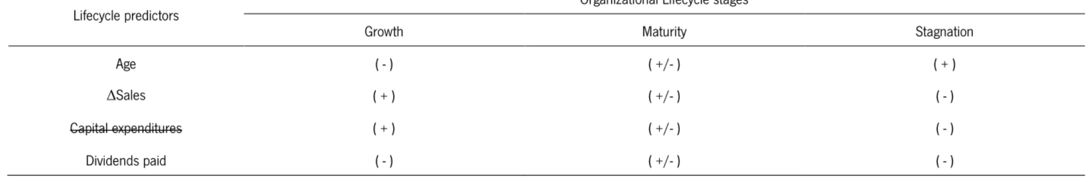
Rather than a single proxy approach, this is a multivariate method that contains variables, frequently documented in similar contexts, as age, capital expenditures, sales variation and dividends paid, all of which, fit perfectly into Mueller’s (1972) hypothesis, and where:

 Age – in years. Since the database was missing the foundation date variable, age was estimated using 1) the incorporation date and 2) the date of entry in the database14. Both

alternatives were used in the past, and not surprisingly, produced similar results.

 Capital Expenditures – capital expenditures as a percentage of total value. Despite being initially considered, this variable was eventually dropped and not used during the classification stage, since it can bias the classification of growth firms. As explained in Anthony & Ramesh (1992), some sectors show higher levels of capital expenditures than others, and firms in those sectors aren’t necessarily in growth stages.

 Sales variation – as percentage sales growth.

 Dividends paid – common dividends as a percentage of net income before extraordinary items and preferred dividends.

The logic behind each of these variables is very straightforward. Firms in growth stages should, on average, be younger, show higher sales growth and pay less, if any, dividends. Also, as they evolve, the relationships should reverse as shown in Table 6.

(25)

24

After sorting out the variables that are used as life stage predictors, the following few steps were involved, in order to reach a final classification:

 Calculate each predictor for every firm year in the sample;

 For each firm year, compute a five years mean of each of the predictors15;

 Rank each firm year according to each predictor mean, and group them into three quantiles.

 Give a partial score, ranging from 1 to 3, to each predictor mean, in accordance with the quantile occupied.

 Calculate a final composite score, given by the sum of the partial scores. Considering the lowest and highest scores in all three descriptors we know that the composite score can fluctuate between 3 and 9.

 Finally, assign a firm life stage based on the composite score, as shown in Table 7.

While the organizational life cycle theory is widely accepted, some researchers16 still discuss whether its

applicability is limited, sustaining their criticism on an eventual lack of support for a sequential progression between stages. In fact, already in the middle 60s, Gardner (1965) was sympathetic with this issue, when he writes that “organizations differ from people and plants in that their cycle isn’t even approximately predictable. An organization may go from youth to old age in two or three decades, or it may last for centuries. More important, it may go through a period of stagnation and then revive”. (Gardner, 1965, p.16)

That is one serious pitfall in which univariate (i.e. by age) classifications can easily incur. However, the multivariate system described earlier, does not solely constrain the maturity stages to time, thereby accomplishing two goals. First, regarding the problem of linear assignment of stages, where a mature

15_{This step enforces that each firm in the sample contains at least 6 years of consecutive data, prior to each firm year.}

16_{i.e., Churchill & Lewis (1983), Scott & Bruce (1987), O’Farrell & Hitchens (1988), Kazanjian & Drazin (1989), McMahon (2001), Lester et al. (2003),}

(26)

25

or even stagnant stage can precede a growth stage, as long as that particular firm observation displays other growth characteristics (i.e. high sales, low dividends). Secondly, the use of multiple variables should mirror more precisely the various changes that firms endure at each stage, increasing the reliability of the process.

To summarize, measuring and assigning stages of maturities is a complex task prone to errors of various sorts. Nevertheless, we find the methodology adopted especially flexible and adequate for its purpose.

(27)

26

4 - Sample and Data

All the accounting information was obtained from the international data bases – Datastream and Worldscope. The initial dataset, comprising data for firms from 31 industrial subsectors17 and all 49

countries18 listed in La Porta et al (1997), for the broadest period available (12 years), was properly

standardized19.

To ensure data validity and integrity, numerous sanitizing procedures and rules were applied. All non-industrial firms (i.e., financials, and regulated utilities) as well as firm repetitions20 were automatically

discarded. Other factors that could compromise the inclusion of a given firm included the occurrences of invalid and/ or insufficient data to compute the necessary summary variables, listed in appendix A, or the variables used to separate firms into different stages of maturity.

After completing the elimination process, all variables are winsorized at 5% to mitigate the adverse effects of outliers and the final sample is left with 12,235 firms and 56,420 valid firm observations between 1996 and 2007. While the date of 1996 imposed itself because of technical limitations (not enough data and/or firms for previous years), the date of 2007 was deliberately chosen to avoid a well-known period of world economic crisis that could lead to incorrect results21.

Also, because it’s not uncommon to find that similar studies often end with different results, only because of plain sample diversity22 and the use of different data structures23, all the 56,420 firm

observations are rearranged into different data panels and groups as shown in Figure 1. This way, following a similar intuition as La Porta et al (1997), instead of extracting a single USA sample, the observations are also sorted by country into two additional logical groups – Common Law and Civil Law. Withal, two types of data panels are created – Balanced and Unbalanced. Table 1 and Table 2 provide an insight about the countries comprising each sample.

17_{Following standard practice, all the sectors known to operate under special regulations are excluded (i.e., Financials, regulated utilities).} 18_{Except Uruguay which no longer seems to be part of the data base.}

19_{All the information was converted to 2007 dollars and deflated using the appropriate ICP (index consumer price).} 20_{Firms with various stock emissions will be double listed in the worldscope data base.}

21_{As far as this paper is concerned, crises are exceptions, not the rule. Sporadic events, that place firms under exceptional conditions of financial distress.}

This fact alone, could seriously compromise the performance of both capital structure models.

22_{Studies conducted in different countries.}

23_{Balanced or unbalanced data panels. This is important because balanced panels lead to problems of survivorship bias, where only firms that exist for}

(28)

27

Finally, due to insufficient firm observations in the balanced samples, only unbalanced samples are further refined into three distinct stages of the organizational life cycle namely, growth, maturity and stagnancy.

In the end, a total of 15 samples, that should help better understand just how randomly the trade-off and pecking order models, described in Section 3, perform under different scenarios, and more importantly, with firms in different stages of maturity.

4.1 - Characteristics of Samples

Opting for balanced panels in detriment of unbalanced ones has important repercussions. By definition, a balanced panel imposes that a firm cannot have any year gap during the whole observation period. In Table 3, we can see that this constraint alone causes both a significant reduction in the number of observations, and a slight skew in the composition of the samples, at the industry level24. More

precisely, enforcing this rule diminishes the exposure of the samples to firms in sectors generally associated with growth opportunities (i.e., technology, healthcare).

Additional peculiarities of the balanced samples are highlighted in Table 5. Taking the USA samples (1) and (4) for instance, we realize that firms contained in the balanced panel (1) are, in average, older (Age), bigger (Size) and more profitable (ROA) than firms in the unbalanced panel (4). Also, the first, tend to pay more dividends (Dividends), display higher tangibility (Tang.) and experience lower sales growth (Δ Sales) than the second. Overall, the same is true for the common and civil law samples (2 and 5; 3 and 6) suggesting that the balanced panels are biased towards older firms. Also, commonly used proxies for growth opportunities including the market to book (MB) and the retained earnings ratio (RE/TA)25, show that while balanced panels are mainly composed of older firms, they’re not necessarily

in a more mature stage (usually characterized by slower growth) since they exhibit similar MB ratios as the unbalanced samples.

24_{Omitted chi-square goodness of fit tests, show that all the balanced and unbalanced samples, as well as the respective subsamples, are composed by}

significantly different percentages of industries (at 1% level).

25_{According to DeAngelo, DeAngelo & Stulz (2006), firms in a capital infusion stage will show a lower RE/TA ratio, while a high ratio will often be a sign}

(29)

28

Turning our attention to unbalanced panels, if we contrast the unbalanced samples in Table 3 with their respective growth, mature and stagnant subsamples in Table 4, we can evaluate just how effective the classification procedure was from an industry point of view. Consistently, the composition of all growth subsamples shift towards Technological and Health sectors, while for mature subsamples the opposite happens, and industries like Services & Goods, Retail, and Construction & Material, move up in the pyramid. Concurrently, in the stagnant subsamples, we can observe how many of the top 5 industrial sectors present in the growth subsamples give place to sectors as Chemicals, Basic Resources, Media, and so on. Altogether, this configuration foreshadows an optimistic classification of firms by stages of maturity that propagates to Table 5, where all the variables contemplated by the organizational life cycle hypothesis (i.e. Age, Size, Δ Sales, MB, Dividends, etc.), behave as one would expect.

Further analysis of Table 5 shows that the most significant net equity issues are carried out by growth firms. Reporting equivalent findings, Fama & French (2002) and Frank & Goyal (2003), argue that from a pecking order perspective, this may pose a conundrum. They reason that, in contrast to mature firms which benefit from an increased diversification as well as a better reputation in debt markets, high-growth firms, usually undergo higher information asymmetry costs. Therefore, one would expect that firms of this nature would follow more diligently a theory that rests on the idea that, adverse selection problems are the engine empowering firms’ financial decisions – pecking order- which does not occur in their results.

Despite compromising the strict pecking order theory, another story tells, according to Lemmon & Zender (2010), that equity issues by high-growth firms are in fact contemplated by the weak-form of the pecking order theory. Not only that, but they also point out why high-growth firms may not be subject to higher asymmetry costs than their mature counterparts. One interpretation posits that the higher asymmetry regarding its assets in place is in reality overshadowed by the superior value of their growth opportunities. Additionally, they claim that the reduced debt capacity of smaller firms attenuates the negativity that is usually signaled together with the announcement of an equity issue, when investors realize their lack of financial alternatives.

(30)

29

Moving on to the book leverage, it does not seem to follow any clear pattern. In fact, with the exception of the USA samples, it’s not even statistically different26 between most stages of maturity and when it is,

the values are still very similar. A plausible reason could be the conflicting relation between leverage and the organizational life cycle hypothesis. As we discussed earlier, according to the organizational life cycle hypothesis, as firms evolve from younger to more mature stages, growth opportunities (MB) tend to decrease while profitability (ROA) increases and vice-versa. However, together with other proxies, MB and ROA are also part of a well-documented set of variables that are correlated with leverage. In particular, according to Rajan & Zingales (1995), Fama & French (2002) and Frank & Goyal (2009) leverage is negatively related to both. A relation for which we also provide evidence in Table 11, where after a common leverage regression, we find negative statically significant coefficients between leverage and both ROA and MB. In practice, this means that at any given stage they will be exerting opposite effects on leverage, explaining the homogenization present in Table 5.

One puzzle where the negative relation between ROA and leverage fails to fit is the trade-off theory, and could anticipate an overall inadequate fit of the trade-off as a valid capital structure theory to our samples. All the same, it’s worth mentioning that this already poses an early hindrance to the optimum capital structure theory.

(31)

30

5 - Results

In this section we discuss how the trade-off and pecking order models perform with our set of samples. Note that, even though tables present variables scaled by total assets, alternative scales were tested (net assets, sales, total debt + market equity) attaining similar results. Similarly, alternative non-reported dependent variables included the use of total debt, besides the long term debt. Also, common econometric disturbances as heteroskedasticity, cross-sectional and serial correlation are not left to chance. For that purpose, White, Breusch-Pagan and Wooldridge tests are performed and standard errors have been corrected accordingly. Finally, intending to control for firms specific uniqueness’s we conduct both a (OLS) fixed and a (GLS) random effects analysis. Considering that subsequent Hausman tests27 account for significant differences between the two approaches, only the fixed effects

estimations (simultaneously controlling for firm and time - year-) are reported.

5.1 - Trade-off Theory

The results for the trade-off and pecking order models are conveniently separated into different tables. Starting with the trade-off in Table 8, ΔLD denotes the dependent variable (Variation of long term debt ratio) and Target deviation 1 and Target deviation 2, two substitute definitions for the independent variable (target debt ratio deviation). As in Shyan-Sunder & Myers (1999), they are historic debt ratio means, but while the first is a five-year rolling average, the second is an average for the full period by which a firm enters the sample. A third specification regarding an industry average of debt ratios was also tested but, like Target deviation 1, although statistically significant, proved to be a weak proxy, with low adjustment coefficients and poor predictability. Target deviation 2, on the other hand, provides moderate support for the trade-off theory, with much better results where the adjusting coefficients and R2 are as high as 0.523 and 28,6% (unbalanced common law sample). These results are in line with

the ones presented by Shyan-Sunder & Myers (1999).

27_{Wooldridge (2002) explains that “since FE is consistent when ci and Xit are correlated, but RE is inconsistent, a statistically significant difference is}

(32)

31

A quick comparison of results, both within and between panels, indicates that the trade-off performs considerably better with our set of unbalanced samples where the adjustment factors and predictability are factored by a 50% increase. Take for instance, the balanced Common Law sample (β=0.346, R2=21.8%) and the unbalanced Common Law one (β=0.523, R2=28.6%). Moreover, one should note

that the adjustment coefficients in the balanced samples range from β=0.323 to β=0.370 while in the unbalanced samples from β=0.471 to β=0.523. Clearly, there is a more substantial variance in coefficients between samples of different data panels. This is a strong indication that firm specific characteristics (i.e. age, size, market-to-book, tangibility, etc.) play a major role in the financial decisions as opposed to other exogenous factors (geographically related). Particularly in this case, the trade-off shows a certain affinity to firms that show characteristics often recognized in younger firms (unbalanced samples).

In Table 9, we have our unbalanced samples (USA, Common Law and Civil Law) split into different maturity stages. This time, the variable Target deviation 1 was foregone in consequence of its poor results during previous tests. Our results show, that the trade-off model exhibits a consistent tendency throughout all the samples used. Coherent with our previous findings, where the trade-off performance was slightly better with the unbalanced samples (more exposed to younger firms), also here, we see that the coefficients are constantly higher for firms in growth stages and degrade nearly 14%, on average, as we progress to mature stages.

At stagnancy, there are some obvious differences, however. While the USA and Common Law samples, show similar coefficients for firms in the mature and stagnant stages, the Civil Law stagnant subsample stands out with a strikingly high coefficient, matching the ones observed only in growth firms.

Performing a similar analysis on Table 10, now using interaction variables for the maturity stages, as well as additional control variables (size, tang, roa and mb) to better isolate the effect of Target deviation 2, we find that the adjustment coefficients remain highly significant in all stages. Also, the generalized tendency continues to be characterized by a statistically significant degeneration of the trade-off results as we advance past growth stages, common to all the samples but the Common Law, where the coefficients linger around β=0.560. Overall, with coefficients oscillating between β=0.410 and β=0.579, our results reasonably seem to support the idea that firm’s leverage is mean reverting, at least, partially.

(33)

32

To further assess the degree of the adjustment we also present Table 12, Table 13 and Table 14, where Flannery & Rangan’s (2006) framework is used. Table 12 shows that the correlation indexes between variables range from -0.414 to 0.450, confidently alleviating any concerns about multicollinearity. In Table 13, we perform 3 different estimations.

As Flannery & Rangan (2006) mention in their work, the correlation between the independent variable LMLR (lagged market leverage ratio) and unobservables relegated to the error term, generates a problem of endogeneity, which in turn leads to overestimated adjustment coefficients (columns 1, 3 and 7). A method to deal with unobserved effects involves using fixed effects estimators (within regressions) that tend to perform well when the explanatory variables are strictly exogenous. However, due to endogeneity, this approach is also unfeasible and will often result in a downward bias of the estimates (columns 2, 4 and 8). Essentially, this means that the true adjustment speeds will be somewhere in between the estimates of the GLS (random effects) and OLS (fixed effects) regressions. One solution to mitigate the problem of omitted variables bias and finding the true estimates consists in using instrumental variables. Thus, we conduct a two-stage least squares regression (columns 3, 5 and 9) where the lagged book leverage ratio (LBLR), calculated as total debt to book value of assets, is used as an instrument for the lagged market leverage ratio (LMLR). LBLR displays a correlation of 89% with LMLR in the USA and Common Law samples, and 90.14% in the Civil Law sample (Table 12).

As expected, the new estimates for LMLR land between the ones computed previously. In Table 13, we report statistically significant adjustment speeds of 54.3% for the USA, 52.3% for the Common Law and 50.4% for the Civil law samples. Despite the similitude of coefficients, these results also show some degree of consistency with the view that legal environments that benefit from stronger investor protections as well as more developed capital markets, contribute to raise the willingness to exchange funds for securities (La Porta et al., 1997). This could explain why firms in the USA adjust their capital structure 3.9% faster than firms in Civil Law countries.

Moreover, in Table 14, we find that growth firms adjust faster than mature or stagnant firms. In fact, the Common Law and Civil Law growth samples adjust approximately 13% faster than the mature ones, displaying adjustment speeds as high as 64.5% (Common Law). Curiously, while the USA growth

(34)

33

samples display a slower adjustment speed of 60.7%, the mature USA firms, adjust 6-7% faster when compared to the Common Law or Civil Law counterparts.

Summing up the trade-off evidence provided so far, we believe that, despite some theoretical inconsistencies, this theory remains a strong contestant, empirically. Also, through the lens of the organizational life cycle hypothesis, we can confidently argue that firms financing decisions are not stage invariant either in amount or speed.

5.2 - Pecking Order Theory

Regarding the pecking order in Table 15, ΔLD is used as the dependent variable (variation of long term debt) and Deficit 1 and Deficit 2 as explanatory variables, representing the financial needs of a given firm. Here, Shyan-Sunder & Myers (1999) propose that the Deficit 2 is computed as the sum of dividends paid, capital expenditures, current portion of long term debt and increase in working capital, minus the net cash flow from operating activities. Frank & Goyal (2003) disagree, alleging that the current portion of long term debt does not belong in the equation and thus outlined Deficit 1, where CPLT (current portion of long term debt) is left out. Further illustrating Frank & Goyal’s (2003) critique, all columns in Table 16 show that ΔLD and CPLTD are inversely related (negative coefficients), meaning that any increase in the current portion of long term debt, leads to a decrease in long term debt issues, which contradicts the logic behind Deficit(2). Also, contrasting both approaches, Deficit 1 does provide, uniformly, slightly better results for all the samples. Nevertheless, despite the best effort, the coefficients achieved in our tests, using these two methods, are far less supportive of the pecking order than the ones presented in Shyan-Sunder & Myers (1999), with only β=0.373 and R2=27.3%

(balance civil law).

In Table 17, resorting to Fama & French (2005) accounting identity we defined Deficit 3 as the sum of the change in stockholder’s equity and the change in total liabilities, that proved to be a clear improvement over Deficit 1 and Deficit 2, especially concerning the predictability of the model. This time, while we found a similar β=0.398, the proportion of variance in the amount of debt issued, that can be explained by the Deficit3, doubled to 51.6% (balanced civil law). Despite the improvement,

(35)

34

support for the pecking order theory, is still dubious since, for every unit increase in the deficit only 19.7% to 39.8% is issued as debt, evidencing that equity is still a common choice among firms. The magnitude of these findings jeopardizes the arguments behind the pecking order, even if we consider the weak-form of this theory. This interpretation is transversally true for all the samples. The pecking order seems to explain the Civil law samples more accurately when compared to the USA or Common law samples but, the coefficients are disturbingly lower than expected by the theory. Also, returning to Table 11, and running a second leverage regression (columns 2 5 and 8), where we add the Deficit 3 as an explanation variable, does not wipe the effect of other conventional variables. In fact, it’s only statistically significant in the Common Law leverage regression and the impact is rather residual, meaning that while not insignificant, for itself, cannot explain leverage.

An interesting contrast with the previous theory is how the pecking order describes more closely our panels of balanced samples (containing older firms) as opposed to the unbalanced ones. Furthermore, while the coefficients of the balanced samples continue to display a certain similitude, the same does not happen with the unbalanced samples, where they oscillate between β=0.197 and β=0.337. Switching over to Table 18, this erratic behavior becomes slightly corrected and a thin trend starts to emerge among the growth and mature stages. Although less evident in the Civil Law subsamples, the coefficients still improve over the life cycle of the firm. Control variables added later, in Table 19, do not seem to disturb the previous results considering that, the USA and Common Law samples continue to display statistically superior (although still poor) coefficients at mature stages. Apparently evading this trend, the Civil Law results are found to be rather similar between all the maturity stages, possibly highlighting firm’s difficulties to shorten the gap of information asymmetry between managers and investors, even at later stages, which in this case, could be aggravated by the weaker investor’s protection and unsophisticated markets, inherent to civil law legal systems. These largely disappointing results of the pecking order could also suggest that the proxies used to factor in the different organizational life cycle stages, are not tightly related to the performance of the pecking order model. To answer this question and understand what factors are really driving the pecking order results, we follow a more conventional route and desegregate the organizational life cycle stage predictions by grouping the 56,420 firm observations into three quantiles, one variable at a time, until all the variables described in Table 5 are used. Then, we re-ran the pecking order tests for all the groups, in order to

(36)

35

pinpoint which variables produced, simultaneously, the worst and best results in the first and third quantiles or vice-versa. In this manner, we are able to evaluate how the pecking order model reacts when exposed to each individual aspect, namely age (Age), size (Size), dividends paid (Dividends), change in sales (Δ Sales), capital expenditures (Capex), tangibility (Tang), tobin’s q (Tobq), profitability (ROA), change in assets (Δ Assets), Market to book (MB) and retained earnings to total assets (RE/TA). After trying each factor individually as well as several combinations of proxies28, we realize that our

suspicions were right and the proxies used to map the different life cycle stages are not the most critical regarding the pecking order’s model performance. The most pertinent results are condensed in Table 20 where we find that a classification by tangibility (Tang) and size (Size) simultaneously, influence the pecking order tests the most, with special relevance for tangibility alone. It’s worth noting that, after retesting the pecking order model with this new configuration, the coefficients seem to be much more uniform across different samples, performing increasingly better for firms with higher tangibility and size (Q3). But do these findings make any sense regarding the pecking order theory? Actually, these results could help shed some light on why the pecking order seems to break down, especially when high-growth firms are included. To a firm, tangible assets can be described as those which have a physical form. To an investor, tangibility means collateral. If we assume that the pecking order premises are correct, while a firm would prefer to consume debt before equity, in reality, debt, either in the form of loans or bonds, can be blocked and collateral could be decisive to unlock that door.

Banks, in essence, are extremely risk averse, generally conducting thorough due diligence, demanding high collateral and putting firms under strict covenants, before any loan is conceded. Bonds on the other hand, are more flexible but tapping the bond market for the first time also poses some challenges. For a successful issue, a firm would need to be rated by a credible agency and already familiar to the investors base. In such a context, the financing behavior of younger firms may be explained by need instead of choice. Odds are that this kind of firms lack sufficient internal resources to finance their accelerated growth. Investors are not acquainted with them, and banks will often recognize that their tangible assets -collateral- is insufficient to accommodate the risk in which they

28_{The combination of multiple proxies was achieved using a compound score similar to the one described in section 3. For each factor, an additional}

variable was created containing the index of the quantile occupied by each firm observation. Summing these individual indexes, allows the ranking of firm observations into new quantiles, taking into account multiple variables.

Trade-off vs pecking order : a life cycle of financing decisions

Carlos Manuel Alves Domingues

Universidade do Minho

Escola de Economia e Gestão

Trade-off vs. Pecking order:

A life cycle of financing decisions

Dissertação de Mestrado

Mestrado em Finanças

Trabalho realizado sob a orientação do

Professor Doutor Artur Rodrigues

Carlos Manuel Alves Domingues

Universidade do Minho

Escola de Economia e Gestão

Trade-off vs. Pecking order:

Declaração

Agradecimentos

Trade-off vs. Pecking order:

Um ciclo de vida de decisões de financiamento

Resumo

Trade-off vs. Pecking order:

A life cycle of financing decisions

Abstract

Table of Contents

Table of Figures

Table of Tables

1 - Introduction

2 - Previous Research

3- Methodology







4 - Sample and Data

5 - Results