Identification of iberian large fires climate conditions

UNIVERSIDADE DE LISBOA

FACULDADE DE CIÊNCIAS

DEPARTAMENTO ENGENHARIA GEOGRÁFICA, GEOFÍSICA E ENERGIA

Identification of Iberian large fires climate conditions

Inês dos Santos Vieira

Mestrado em Ciências Geofísicas

Especialização em Meteorologia e Oceanografia

Dissertação orientada por:

Professor Doutor Ricardo Machado Trigo

Doutora Ana Cristina Machado Russo

Identification of Iberian large fires climate conditions

Acknowledgements

Firstly, I want to thank my two advisors, Ana and professor Ricardo, for all their advice, availability, patience and support during this journey.

Thanks to all colleagues in the lab 8.3.15. In particular to Miguel for his help in the initial data processing and Python's tips, to Sílvia for being always available and to Virgílio for his advice during the writing of the dissertation.

A very important and special thank you to my parents for always accompanying and supporting me during all phases of this academic career. Thank you very much.

Finally, this work was partially supported by national funds through FCT (Fundação para a Ciência e a Tecnologia, Portugal) under project IMPECAF (PTDC/CTA-CLI/28902/2017).

Identification of Iberian large fires climate conditions

Resumo

Os incêndios florestais são um risco que não é recente na Península Ibérica. No entanto, é inquestionável que alguns dos episódios mais dramáticos, tanto em termos de vítimas infligidas como de área total ardida, ocorreram durante este século, particularmente na região Oeste da Península Ibérica. A sua ocorrência é responsável, todos os anos, por uma grande quantidade de área ardida, traduzindo-se com frequência em impactos humanos e socioeconómicos significativos. Como tal, existe um reconhecimento crescente que a identificação de uma multiplicidade de padrões de circulação associados à ocorrência de fogos (Fire Weather Types, FWT) tem um interesse considerável em estudos de regimes de fogo, nomeadamente para 1) uma melhor compreensão da relação entre a meteorologia e a ocorrência de fogos; 2) explicar os padrões de severidade dos fogos; 3) melhorar as projeções/previsões e estratégias de combate aos fogos.

Neste estudo propõe-se a identificação e a análise dos fatores meteorológicos que controlam as variações da atividade associada aos grandes incêndios na Península Ibérica. Para isso, procede-se à classificação dos grandes de incêndios (aqueles cuja área ardida é superior ao percentil 95) para uma estação de fogos estendida (maio a outubro) para quatro regiões com regimes de fogo semelhantes. A identificação dessas regiões é feita de acordo com as condições meteorológicas locais (temperatura, humidade relativa, velocidade do vento e índices representativos da secura dos combustíveis), recorrendo-se a uma análise de compósitos para diferentes escalas temporais e de forma a captar a variabilidade interanual, subsazonal e sinótica. Para além disso, pretende-se ainda utilizar a análise de clusters (K-means) para identificar um conjunto limitado de FWT, sendo cada um caracterizado por uma certa combinação de condições meteorológicas sinergéticas condutoras do fogo.

A identificação dos limiares a partir dos quais um determinado fogo se considera um grande incêndio em cada uma das quatro regiões da Península Ibérica, permitiu a identificação de limiares distintos, sendo a região Este aquela que apresenta o valor mais elevado (171 ha).

A análise de compósitos aplicada a uma escala diária para as anomalias standardizadas das variáveis meteorológicas e para os índices que funcionam como proxies de seca, tendo em conta os percentis 1, 85, 95, 98 calculados para as áreas queimadas associados aos eventos ocorridos em cada uma das regiões, permite verificar um aumento das anomalias (em módulo) com o aumento da área queimada dos incêndios. A uma escala de 12 dias, as variáveis meteorológicas são aquelas que têm maior importância na distinção da atividade associada aos grandes incêndios, embora com desfazamentos (lags) temporais diferentes para as quatro regiões. A uma escala mais longa (oito meses), os índices que traduzem a secura dos combustíveis a diferentes camadas do solo são aqueles que têm maior importância.

A aplicação da análise de clusters permitiu identificar três FWT distintos para cada uma das regiões. O FWT_1 caracteriza-se por anomalias da velocidade do vento elevadas (acima de um desvio padrão). No caso do FWT_2, as anomalias das variáveis meteorológicas são bastante menores, situando-se abaixo de um desvio padrão. Por fim, o FWT_3 distingue-situando-se por apresituando-sentar elevadas anomalias da temperatura e humidade relativa (acima de um desvio padrão). As quatro regiões apresentam, no entanto, resultados diferentes para cada um dos FWT identificados. Para além disso, verifica-se que o FWT_3 é aquele a que estão associadas as condições de secura dos combustíveis mais intensa para todas as regiões.

Identification of Iberian large fires climate conditions

A uma escala de 12 dias, verifica-se que: 1) para o caso do FWT_1 a influência do vento está restrita ao dia do fogo; 2) para o FWT_2 as anomalias variam em torno de zero sem nenhum padrão definido; 3). O FWT_3 não apresenta uma influência restrita ao dia do fogo, mas a sua influência varia nas quatro regiões.

A análise do estado da secura dos combustíveis associados aos eventos caracterizados por cada um dos FWT permitiu identificar que o FWT_3 é aquele a que corresponde a uma situação em que os os índice representativos da secura dos combustíveis apresentam anomalias mensais mais elevadas quando comparadas com as anomalias do FWT_1 e FWT_2 para as quatro regiões.

Esta análise permitiu identificar as condições climáticas associados à ocorrência dos grandes incêndios para quatro regiões da Península Ibérica tendo em conta as características meteorológicas das regiões, permitindo assim, diferenciar as condições meteorológicas e as diferentes escalas temporais entre a atividade que está na origem de todos os incêndios e aquela que está associada aos grandes incêndios.

Identification of Iberian large fires climate conditions

Abstract

The Mediterranean region is characterized by the frequent occurrence of summer wildfires representing an environmental and socioeconomic burden. Some Mediterranean countries (or provinces) are particularly prone to Large Fires (LF), namely Portugal, Galicia, Greece, and southern France. On the other hand, the Mediterranean basin corresponds to a major hotspot of climate change, and anthropogenic warming is expected to increase the total burned area due to fires in Mediterranean Europe.

Here, we propose to classify summer large fires for four regions of Iberia (with similar fire regimes) according to their local-scale weather conditions (i. e. temperature, relative humidity, wind speed) and fire danger weather indices (Duff Moisture Code and Drought Code). The composite analysis was used to investigate the impact of local and regional climate drivers at different time scales, and to identify distinct climatologies associated with the occurrence of LF in Iberia for an extended fire season (May to October). A Principal Component Analysis (PCA) was applied to identify the variables with the highest variance explained for the fire day. Also, cluster analysis was used to identify a limited set of Fire Weather Types (FWT), each characterized by a combination of meteorological conditions leading to a better understanding of the relationship between meteorology and fire.

For each of the regions, three FWTs were identified with different characteristics. The FWT_1 is characterized by high anomalies (above one std) of zonal wind velocity. The FWT_2 presents anomalies of the meteorological variables within the average (bellow one std). Finally, the FWT_3 is categorized by high positive temperature anomalies (above one std) and strong negative relative humidity anomalies (bellow one std). The methodology followed allowed to objectively identify for different regions of Iberia multiple fire climatologies associated with the occurrence of LF.

Identification of Iberian large fires climate conditions

Index

Acknowledgements ... II Resumo ... III Abstract ... V Table of figures ... VII List of tables ... VIII List of abbreviations and symbols ... IX

1. Introduction ... 1

2. Data ... 3

2.1. Rural fires ... 3

2.2. Meteorological variables ... 4

2.3. Fuel moisture codes ... 5

3. Methodology ... 8

3.1. Large fires classification ... 8

3.2. Composite Analysis ... 9

3.3. Principal Component Analysis (PCA)... 9

3.4. K – Means algorithm ... 11

4. Results and Discussion ... 13

4.1. Characterization of the study area ... 13

4.2. Large fires classification ... 14

4.3. Composite Analysis ... 16

4.3.1. Day of fire ... 16

4.3.2. Twelve days ... 19

4.3.3. Five Weeks ... 20

4.3.4. Eight months ... 22

4.4. Principal Component Analysis ... 23

4.5. K – Means Analysis: Fire Weather Types identification ... 24

4.6. Fire Weather Types characterization ... 27

4.6.1. Twelve days ... 27

4.6.2. Eight months ... 29

5. Conclusions ... 30

6. References ... 33

Identification of Iberian large fires climate conditions

Table of figures

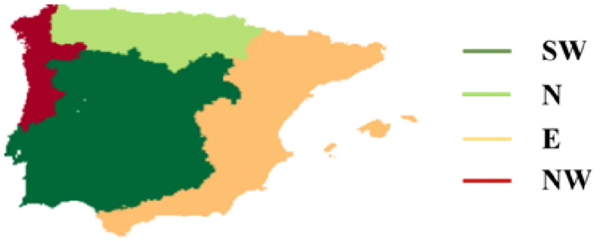
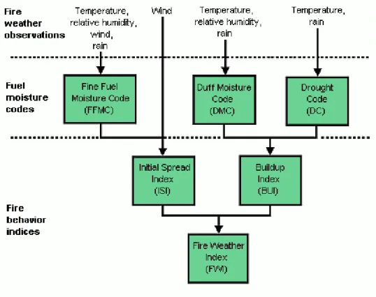
Figure 2.1. - Geographical boundaries of the four spatially homogeneous regions of IP: Southwest (SW), North (N), East (E) and Northwest (NW). ... 5 Figure 2.2 – Schematic representation of the structure of the Fire Weather Index (FWI) system. Source: CWFIS. ... 6 Figure 3.1 – Summary of the Principal Components Analysis Approach. ... 11 Figure 4.1 - Monthly average values of temperature (⁰C), relative humidity (%), zonal wind (m/s), meridional wind (m/s) and precipitation (mm) for the four regions: Southwest (SW), North (N), East (E) and Northwest (NW). ... 13 Figure 4.2 - As in Fig. 4.1 but for DMC and DC. ... 14 Figure 4.3 - Percentage of burned area during the months of May, June, July, August, September and October for the four regions. ... 14 Figure 4.4 - Representation of the following representative percentiles: 1, 85, 95 and 98 for the four regions. ... 15 Figure 4.5 - Interannual variability of the number of large fires per year observed in the four considered regions. ... 16 Figure 4.6 – Composites of standardized anomalies of temperature, relative humidity (RH) and zonal velocity of the wind (U) of the day of fire for the SW, N, E and NW regions according to the percentiles 1 (gray), 85 (purple), 95 orange), 98 (red) of the final burned areas. ... 18 Figure 4.7 – As in Fig. 4.6 but for DMC and DC. ... 18 Figure 4.8 - Composites of standardized anomalies of temperature, relative humidity and zonal wind velocity at 12 days for all fires (gray) and for large fires (red) for regions under study. ... 19 Figure 4.9 - As in Fig. 4.8 but for DMC and DC. ... 20 Figure 4.10 - Composites of standardized anomalies of temperature, relative humidity and zonal wind velocity at 5 weeks for all fires (gray) and for large fires (red) for the regions. ... 21 Figure 4.11 - As in Fig. 4.10 but for DMC and DC. ... 21 Figure 4.12 - Composites of the monthly standardized anomalies for eight months temperature, relative humidity and zonal wind velocity for all fires (grey) and for large fires (red). ... 22 Figure 4.13 - As in Fig. 4.12 but for DMC and DC. ... 23 Figure 4.14 – Explained variance for the six principal components (PC 1 through PC 6) corresponding to the temperature (red), relative humidity (green), wind direction (blue), DMC (black), DC (pink) and precipitation (yellow) for the four regions of Iberia. The dashed blue line symbolizes the cumulative explained variance. ... 24 Figure 4.15 - Composites of the standardized anomalies of the meteorological variables (temperature, relative humidity and zonal wind) of the fire day associated with the three Fire Weather Types identified by K-means, FWT_1 (blue), FWT_2 (green) and FWT_3 (red). ... 25 Figure 4.16 - As in Fig. 4.15 but for DMC and DC. ... 26 Figure 4.17 - Composites of the standardized anomalies of the meteorological variables (temperature, relative humidity and zonal wind) at 12 days timescale associated with the three Fire Weather Types identified by K-means, FWT_1 (blue), FWT_2 (green) and FWT_3 (red)... 28 Figure 4.18 – As in Fig. 4.17 but for DMC and DC. ... 28 Figure 4.19 - Composites of the standardized anomalies of DC and DMC at 8 months timescale associated with the three FWT. ... 29 Figura A.1 – Trends of FWT_1 annual number of large fires (Mann- Kendall Test p<0.001) for the SW, N and E with a negative trend and NW with no trend. ... 37 Figure A.2 – Trends of FWT_2 annual number of large fires (Mann- Kendall Test p<0.001) for the SW and NW with a negative trend and N and E regions with no trend. ... 38 Figure A.3 - Trends of FWT_3 annual number of large fires (Mann- Kendall Test p<0.001) for the N and E with a negative trend and NW and SW regions with no trend. ... 39

Identification of Iberian large fires climate conditions

List of tables

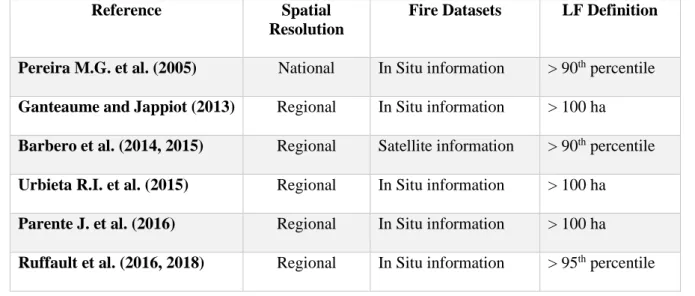
Table 2.1 - Monthly amounts of the empirical Daylength factor used to compute DMC and the Daylenght Adjustment to calculate DC (Wagner, 1987). ... 7 Table 3.1 - Bibliographical references on the spatial resolution used in the studies on the importance of meteorological factors in the development of large fires, the type of databases for the fire event and also the definition of a large fire considered. ... 8 Table 4.1 - Values of representative percentiles: 1, 85, 95 and 98 for the four regions ... 15 Table 4.2 - Representation of the relative importance of the Fire Weather Types identified in each region in terms of the percentage of Large Fires (LF) of the contribution of the respective burned area. ... 27

Identification of Iberian large fires climate conditions

List of abbreviations and symbols

BA Burned Areas

BUI Buildup Index

CWFIS Canadian Wildland Fire Information System

D Present day’s DC

DC Drought Code

DMC Duff Moisture Code

E East Reagion

ECMWF European Centre for Medium-Range Weather Forecasts EFFIS European Forest Fire Information System

EMS Emergency Management Service FFMC Fine Fuel Moisture Code

FWI Fire Weather Index

FWT Fire Weather Types

ha Hectares

ICNF Institute of Nature Conservation and Forests

IP Iberian Peninsula

IPCC Intergovernmental Panel on Climate Change ISI Inicial Spread Index

K log drying rate in DMC

Le Daylenght Factor in DMC

Lf Daylenght Adjustment in DC

LF Large Fires

M Moisture Content after rain in DMC

M0 Moisture Content from previous day in DMC

MARM Spanish Ministry of the Environment, and Rural and Marine Affairs MSG Meteosat Second Generation

N North Region

NGP Normalised Geostationary Projection

NW Northweast Region

P Precipitation

P0 Previous day’s DMC

PCA Principal Components Analysis PE Potencial Evapotranspiration

Q Moisture Equivalent of DC

Q0 Moisture Equivalent of previous day in DC

Qr Moisture Equivalent after rain

r0 Precipitation of latest 24 hours

rd Effective Rainfall, DC

re Effective Rainfall, DMC

RH Relative Humidity

std Standard Deviation

SVD Singular Values Decomposition

SW Southwest Region

T Temperature

U Zonal Wind Component

V Meridional Wind Component

Identification of Iberian large fires climate conditions

1. Introduction

Wildfires are a recurrent natural phenomenon (Bowman et al. 2009) which occurs with varying regularity and severity across almost every biome on Earth (Archibald et al. 2013). The Mediterranean region is characterised by the frequent occurrence of large summer wildfires and constitutes the region where most of the total burned area in Europe occurs, with an average of 4500 km2 _{per year (Turco et}

al., 2017). However, the relevance of wildfires is not homogeneous within the Mediterranean basin, with some specific countries (or provinces) being particularly prone to Large Fires (LF), namely Portugal, Galicia (Spain), Greece, southern France (Trigo et al., 2013; Ruffault et al., 2016; Pinto et al., 2018). Unquestionably, some of the most dramatic episodes occurred during this century, particularly in the western region of the Iberian Peninsula (Sousa et al. 2015), often translating into significant human and socio-economic impacts (Trigo et al. 2013, Sanchéz-Benitez et al., 2018). Numerous features make the landscape of Mediterranean Europe dissimilar from those of the rest of European continent, and these differences are mostly related to the climate and the long and intense impact of humans, but also reflect the role of fire (Pausas and Vallejo, 2011).

In the last decades, the European Mediterranean countries have experienced profound social and economic changes, in particular, the depopulation of rural areas, leading to the abandonment of large areas of cultivated areas which have led to the recovery of vegetation and an increase in accumulated fuel causing an increase in fire frequency (Pereira et al. 2005, Costa et al. 2011). Apart from the social and economic factors, weather and climate play a vital role as a distinguishing factor, so that most fires occurring in Europe occur in the Mediterranean basin. Moreover, most of the fires occur during the summer months, when the high temperatures and the low air humidity and fuel moisture increase the risk of fire (Trigo et al. 2006, Turco et al. 2013, Amraoui et al. 2015, Erickson et al. 2016). Furthermore, according to the latest report by IPCC (SR 1.5, 2018), it is expected an increase in mean global temperatures, including for the Mediterranean Europe area. However, whereas in the Mediterranean regions a decrease in precipitation is projected which has already started to occur (Ozturk al. 2015, Polade et al. 2017), leading to the occurrence of more frequent, prolonged and intense droughts in the Mediterranean, the remaining regions of Europe, especially in the North, an increase in precipitation is expected, and an increase in the occurrence of droughts is not anticipated (IPCC SR1.5, 2018). Besides these differences, the total burned area depends on a multiplicity of another factor, such as topography, biomass production and its availability to burn, ignitions patterns (Archibald et al. 2009).

The role played by climate and weather in LF occurrence has been frequently discussed (Flannigan et al., 2000; Pereira et al., 2005), putting in evidence that they both act at different time scales (Barbero et al., 2015). Ruffault et al. (2016, 2018) describe in details the role of meteorological and climatological variables in the occurrence of fires of different sizes in southern France, showing that at an annual to seasonal time scales, the atmospheric conditions are essential to the growth of the fine fuels. Besides, before and after the fire season, daily to monthly atmospheric conditions are responsible by the changes in moisture content, and finally, the instantaneous conditions (hourly to daily) in meteorological variables may influence fire ignition, intensity and propagation (Riley et al. 2013, Barbero et al. 2015). The dependency of fire activity on meteorological conditions can be quantified using directly meteorological variables or using indices that combining several meteorological variables. Fire danger rating systems try to anticipate periods of heightened fire risk, mainly for early warning to the authorities. One of these systems, most likely the best known in Europe and North America, is the

Identification of Iberian large fires climate conditions

often used to rate the fire danger. The FWI is based on daily values of temperature, relative humidity, wind at noon and 24-hour accumulated precipitation, and has been operational since 1970 in Canada (Van Wagner, 1987) being the most extensive fire danger rating system used operationally in the world (Field et al., 2015).

In Europe, the FWI system is fully operational and is provided every day by the EFFIS (European Forest Fire Information System) which is part of the Copernicus Emergency Management Service (Copernicus EMS). The Copernicus EMS was developed so it “provides information for emergency response in relation to different types of disasters, including meteorological hazards, geophysical hazards, deliberate and accidental man-made disasters and other humanitarian disasters as well as prevention, preparedness, response and recovery activities”. The Copernicus EMS is composed of an on-demand mapping component providing rapid maps for emergency response and risk and recovery maps for prevention and planning and of the early warning and monitoring component which includes systems for floods, droughts and forest fires (Copernicus Emergency Management Service, 2019).

However, there is considerable interest in identifying the meteorological factors that control the variations in LF activity under a global change context, since, there are still few studies on the impacts of climate change on fire risk for the Iberian Peninsula. For example, Sousa et al. (2015) projected for future climate scenarios, an increase in mean burnt areas for the considered pyro-regions of the Iberian Peninsula, with an increase of burned areas that can be two to three times higher than the current one. Whereby there is growing recognition that the identification of a multiplicity of Fire Weather Types (FWT) has a considerable interest in studies of fire regimes, namely for (1) a better understanding of the relationship between meteorology and the occurrence of fires; 2) explain the patterns of fire severity; 3) to improve projections/forecasts and fire-fighting strategies at a regional scale (Ruffault et al. 2016).

This study focuses on the analysis of historical meteorological data and records of fires and it aims to classify large summer fires for four regions of Iberia according to their local-scale weather conditions (i. e. temperature, relative humidity, wind speed) and fire danger weather indices that are components of the Canadian FWI (duff moisture code and drought code). The composite analysis was used to investigate the impact of local and regional climate drivers at different time scales, and to identify distinct climatologies associated with the occurrence of LF in Iberia.

Identification of Iberian large fires climate conditions

2. Data

2.1. Rural fires

Information on each fire event recorded between 1980 and 2015 is taken from two separate databases. For Portugal, it was used the information provided by the Institute of Nature Conservation and Forests (ICNF), and for Spain, the data was provided by the Ministry of Environment, Rural, and Marine Affairs (MARM) of the Government of Spain.

The ICNF rural fire database is not consistent throughout the study period, and the information provided is different (Pereira et al., 2011). Two different periods can be considered, the first from 1980 to 2000, which for each fire includes information about the district, municipality and the parish of the ignition, the date and time of the beginning and the extinction of the fire, the total burned area of the fire in hectares, which corresponds to the sum of the forested areas and non-wooded areas and, finally, the cause of the fire when known. After 2001, the great addition to the previous information is that the “exact” location of the beginning of the fire in XY coordinates was added instead of considering as previously that the fire began in the centre of the parish (Pereira et al., 2011).

The Spanish database is considered one of the oldest in Europe, providing fires data since 1968 (Velez, 2001), though the records are not considered entirely consistent until 1988. All the information included in this dataset is compiled from the information provided by the forest fire reports from the autonomous regions (Moreno et al., 2011). Accurate information about the fire location is only available since 2000, where the utilization of GPS improved the knowledge of fire ignitions. Here the fire ignition documented is based on a spatial reference grid of 10×10 km provided by ICONA, the firefighting services use this grid for the determination of the approximate location of fire events, and moreover, the municipality origin of the ignition is also recorded. The method described by De la Riva et al. (2004) to locate the start of the fires successively refines and decreases the potential location area of the ignition points by excluding areas where the fire could not have occurred. It starts in the 10×10 grid, i.e. with a potential location area of 100 km2_{. Later this area is decreased by intersecting with the frontiers of the}

municipality origin of the fire. Lastly, the location area is restricted to the forest perimeter (MARM, 1997) to determine the final potential location area. The use of this technique leads to a substantially smaller area where the ignition points are then randomly distributed (Rodrigues and De la Riva, 2014). For this study, it is considered a prolonged fire season is spanning between May and October, since, most of the large fires in the Iberian Peninsula occurs during the summer period. The analysis was also restricted to burned areas above 1 ha in order to exclude fires whose development was not forced by meteorological factors. Besides that, the fire events of both datasets are organised by date. Each event is also spatially organised by the 18 districts in Portugal and 48 provinces in Spain (Fig. 2.1).

Afterwards, each fire was associated to one of the four regions identified by Trigo et al. (2013) for the Iberian Peninsula (IP), where a cluster analysis allowed the identification of four spatially homogeneous regions (Southwest (SW), North (N), East (E) and Northwest (NW)) with a similar fire regime (Figure 2.1).

Identification of Iberian large fires climate conditions

2.2. Meteorological variables

The meteorological variables used in this analysis are taken from the ERA-Interim archive (Dee et al., 2011). ERA-Interim is a global atmospheric reanalysis produced by the European Centre Medium-Range Weather Forecasts (ECMWF) and is provided with a sequential data assimilation scheme, ad-vancing forward in time using 12-hourly analysis cycles, where the observations are combined with prior information from the forecast model to estimate the evolving state of the global atmosphere and its underlying surface (Dee et al. 2011). This reanalysis covers the period since 1979 and continues to be updated until 31 August 2019. The ERA-Interim project was developed with the purpose of preparing a future reanalysis covering the whole of the 20th century but the main objectives of the project were to improve some critical features of ERA-40, such as the representation of the hydrological cycle, the quality of the stratospheric circulation, and the handling of biases and changes in the observing system (Berrisford et al. 2011).

The spatial resolution used by ERA-Interim configured for the data set is approximately 79 km (reduced Gaussian grid) on 60 vertical levels from the surface up to 0.1 hPa. The ERA-Interim data assimilation and forecast suite produce four analyses per day, at 00, 06, 12 and 18 UTC and two 10-day forecasts per day, initialised from analyses at 00 and 12 UTC. For detailed documentation of the ERA-Interim archive, see Berrisford et al. (2011) and Dee et al. (2011).

For this study, five daily surface variables at 12 UTC were extracted from the ERA-Interim rea-nalysis database, namely, dewpoint temperature at 2 m, the temperature at 2 m, zonal wind component at 10 m, meridional wind component at 10 m and accumulated precipitation of the last 24 hours. In addition to these variables, the relative humidity was computed from the Magnus formula, depending on dewpoint temperature and temperature at the surface, described by Lawrence (2005).

The wind intensity was calculated from the module of the zonal and meridional wind components for each grid point.

The meteorological data were re-projected in the normalised geostationary projection (NGP) of Meteosat Second Generation (MSG) following Pinto et al. (2018) since the FWI database is calculated for the MSG disk, as well as the respective indexes that give rise to it, including DMC and DC. After-wards, each grid point is attributed to one of the four regions identified by Trigo et al. (2013) for the IP (Figure 2.1).

The meteorological data were then put through a preliminary pre-processing sequence according to the following procedure:

1. Calculation of daily, weekly and monthly climatologies for the mentioned var-iables and using as reference period the years from 1980 to 2015.

2. Calculation of daily, weekly and monthly anomalies for all variables in the study.

Identification of Iberian large fires climate conditions

2.3. Fuel moisture codes

The FWI system is organised into six different components reflecting distinct aspects of the impact of meteorological variables in the fuels flammability and fire spreading characteristics (Figure 2.2). FWI system computation requires measurements of instantaneous temperature at 2 m, relative humidity at 2 m and sustained wind speed at 10 m, all at noon and precipitation totalled over the previous 24 h. Firstly the FWI system computes the fuel moisture codes that follow daily changes in the moisture contents of three different layers of forest fuel with varying rates of drying, in second place is performed the two intermediate components of the system which demonstrating rate of spread and amount of available fuel. Moreover, finally, it is calculated the Fire Weather Index (Figure 2.2). The FWI is an amalgamation of the ISI (Initial Spread Index) that quantifies the rate of spread alone without the influence of variable quantities of fuel, and the BUI (Buildup Index) that accounts for the total fuel available to the spreading fire, indicating the intensity of the spreading fire as energy output rate per unit length of the fire front (Wagner, 1987).

In this study, two codes associated to the BUI calculation were considered in further detail, namely the Duff Moisture Code (DMC) and the Drought Code (DC). Both the DMC and DC are nu-merical values that represent the average moisture content of fuels. In case of the DMC, of the loosely compacted organic layers of moderate depth equivalent, a duff layers about 7 cm deep and 5 kg/m2 _in

dry weight and the primary goal of this code is indicating fuel consumption in moderate duff layers and medium-size woody material. The DMC is computed through the following equation (Van Wagner, 1987):

𝐷𝑀𝐶 = 𝑃 + 100𝐾 (2.1) DMC is computed following a two-stage process. The first one is the rainfall phase, which aims to calculate the actual moisture content that rises with dryness through the following expression:

Figure 2.1. - Geographical boundaries of the four spatially homogeneous regions of IP:Southwest (SW), North (N), East (E) and Northwest (NW).

Identification of Iberian large fires climate conditions

𝑃 = 244.72 − 43.43 ln(𝑀 − 20) (2.2) The computation of the moisture content after rain (M) that is a function of effective rain (re), a

coefficient b which is performed by one of a set of three empirical equations depending on the value of the initial code (P0), and initial moisture content (M0):

𝑀 = 𝑀0+ 1000 𝑟𝑒⁄(48.77 + 𝑏𝑟𝑒) (2.3)

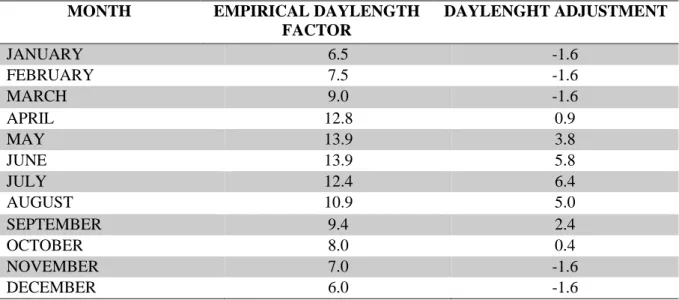
Subsequently, to perform the drying phase, we must compute the log of the drying rate K (given by the following expression) at noon, which is a function of temperature (T) and relative humidity (RH), and also an empirical daylength factor (Le) listed by month in Table 2.1, which is given by the equation:

𝐾 = 1.894 (𝑇 + 1.1)(100 − 𝑅𝐻)𝐿𝑒 10−6 (2.4)

The DC, on the other hand, represents the average moisture content of deep, compacted organic layers and heavy surface fuels, about in average 18 cm deep and 25 kg/m2 _{in dry weight. DC is calculated}

through the following equation Van Wagner, 1987):

𝐷𝐶 = 𝐷 + 0.5𝑃𝐸 (2.5) Where D represents the current drought, and PE corresponds to potential evapotranspiration. As in the DMC, the DC computation involves the calculation of the rainfall phase and the drying phase. The calculation begins with a rainfall phase, which represents the moisture equivalent after rain, which is in the function of the effective rainfall (rd) and the existing moisture equivalent, given by the following

expression:

Identification of Iberian large fires climate conditions

𝑄𝑟 = 𝑄0+ 3.937𝑟𝑑 (2.6)

𝑟𝑑= 0.83𝑟0− 1.27 (2.7)

If the precipitation (r0) of the latest 24 hours it is smaller than 2.8 mm, the component of the

rainfall is ignored for the DC calculation. Therefore, we can perform the calculation of the numerical value of the current drought through the next equation:

𝐷 = 400 ln(800 𝑄⁄ ) (2.8) The drying phase, which is represented through an empirical expression, evaluates the potential

evapotranspiration (PE) depending on the temperature (T) at noon and the seasonal Daylength adjust-ment (Lf) – values at table 2.1:

𝑃𝐸 = 0.36(𝑇 + 2.8) + 𝐿𝑓 (2.9)

The DMC and the DC were both computed using ERA-Interim reanalysis described in the previ-ous section. Moreover, both DMC and DC followed the same procedure described in the previprevi-ous sec-tion for the meteorological variables where it is performed the climatology for the described period, the anomalies (diary, weekly and monthly) calculation and respective standardization of the anomalies to the four regions in the study.

MONTH EMPIRICAL DAYLENGTH FACTOR DAYLENGHT ADJUSTMENT JANUARY 6.5 -1.6 FEBRUARY 7.5 -1.6 MARCH 9.0 -1.6 APRIL 12.8 0.9 MAY 13.9 3.8 JUNE 13.9 5.8 JULY 12.4 6.4 AUGUST 10.9 5.0 SEPTEMBER 9.4 2.4 OCTOBER 8.0 0.4 NOVEMBER 7.0 -1.6 DECEMBER 6.0 -1.6

Table 2.1 - Monthly amounts of the empirical Daylength factor used to compute DMC and the Daylenght Adjustment to calculate DC (Wagner, 1987).

Identification of Iberian large fires climate conditions

3. Methodology

3.1. Large fires classification

There is an extensive bibliography on the meteorological factors that control the activity of large fires (e.g. Vázquez, Moreno J.M. 1995, Kasischke et al. 2002, Bradstock et al. 2009). However, there is no unique definition from which a fire is considered a large fire and different studies use distinct defi-nitions (Table 3.1). While some studies follow official national defidefi-nitions (e.g. Parente et al. (2016) follows the ICNF definition of a LF if the burned area is higher than 100 ha), other studies use statistical definitions (e.g. Pereira et al., 2005; Barbero et al., 2014, 2015). These later consider all those fires with burned areas higher than the 90th percentile of the respective distribution as an LF. Ruffault et al. (2016, 2018) use an even higher threshold, considering that fire is a LF if the burned area is above the 95th percentile of the respective distribution. The use of a percentile based definitions at the national level may not be the correct one, since, a range of factors influences the incidence and size of fires, besides the weather and climate, such as ignition sources, fuels, terrain and suppression forces (Ganteaume et al., 2013). Therefore, the use of a statistical definition should be used for piroregions where fire behav-iour behaves similarly and not based on the borders of a country.

Therefore, following the definition proposed by Ruffault et al. (2016), each fire event was classi-fied into four classes according to the final burned area. Each class is defined by the calculation of percentiles 1, 85, 95 and 98. Thus, within the scope of this work, a fire was considered a large fire if the burned areas, express in hectares (ha), presented a value higher than of the 95th percentile of the respec-tive distribution, which was determined based on all dataset from 1980 to 2015. This definition is applied to the fire events attributed to the four regions under study (Fig 2.1), previously identified with similar fire regimes. In general, a fire regime characterises the spatial and temporal patterns and ecosystem impacts of fire on the landscape. Accordingly, these regions may be distinguished by how often fires typically occur (frequency, fire interval, fire rotation) and vegetation type (or ecosystem), in conse-quence of similar weather and climate patterns. As a result, it is estimated that the threshold from which one considers an LF in each of the regions has a different value.

Table 3.1 - Bibliographical references on the spatial resolution used in the studies on the importance of meteorological factors in the development of large fires, the type of databases for the fire event and also the definition of a large fire considered.

Reference Spatial Resolution

Fire Datasets LF Definition

Pereira M.G. et al. (2005) National In Situ information > 90th _percentile

Ganteaume and Jappiot (2013) Regional In Situ information > 100 ha

Barbero et al. (2014, 2015) Regional Satellite information > 90th _percentile

Urbieta R.I. et al. (2015) Regional In Situ information > 100 ha

Parente J. et al. (2016) Regional In Situ information > 100 ha

Identification of Iberian large fires climate conditions

3.2. Composite Analysis

One of the objectives of this study is the identification and analysis of the meteorological factors that control the variations of the LF activity that occur in the four Iberian regions (Figure 2.1). For this purpose, a similar approach to Ruffault et al. (2016, 2018) was used, i.e. a composite analysis for different temporal scales: twelve days, five weeks and eight months, in order to capture the synoptic, subsazonal and interannual variability, respectively.

After a preliminary treatment of the variables (described at section 2.2, 2.3), and considering the thresholds identified by the calculation of the percentiles of the burned areas for each area, two different subsets were considered for each region of the IP: i) for all the fires and ii) the fires with areas burned above the 95th percentile according to the different periodicities to analyse:

Daily: The daily composites of the variables were performed on a time scale of up to twelve

days. The composites are computed based on the mean of the anomalies for several days. Firstly, the days of the ignitions are identified, and after identifying the day of the beginning of the fires is associated with the anomaly of temperature, relative humidity, zonal wind velocity, DMC and DC. Next, the mean of the anomalies for the identified fire days is calculated. This procedure was adapted for the remaining days, where after identifying itself, each of the days of the fire is calculated the mean of the anomalies for each of the days up to 8 days before and in the two days after the day of the beginning of the fire.

Weekly: The weekly composites of the variables are carried out on a time scale of five weeks.

The same procedure was followed as for daily composites, but in this case, after identification of the fire day the climatological anomaly of each of the variables of the week in which the fire occurs is calculated and the weekly average of every week up to 4 weeks before the event and a week later.

Monthly: The monthly composites of the variables are performed on a time scale of eight

months. Once again, after identifying the fire day, the average of the anomalies of the study variables associated with these days was calculated, but in this case, the monthly anomalies associated with each event was considered, and the average of the monthly anomalies are compiled up to 7 months before the fire month and a month after.

3.3. Principal Component Analysis (PCA)

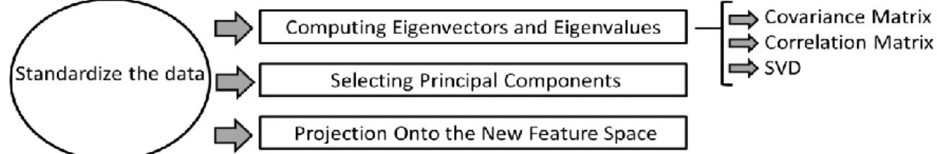
Principal component analysis (PCA) is a statistical procedure where its main objective is to reduce the dimensionality of a dataset consisting of many interrelated variables while retaining as much as possible of the variation present in the data set (Jolliffe, 2002). This is achieved by performing an orthogonal transformation to obtain a new set of linearly uncorrelated variables, the principal components, and which are ordered so that the first few retain most of the variation present in all the original variables. Figure 3.1 is a schematic summary of the PCA approach.

Identification of Iberian large fires climate conditions

The PCA method is widely used in many scientific fields of study such as in agriculture (Nikkhah et al. 2019), chemistry (Malik et al. 2018), climatology (João A. Santos and Margarida Belo‐Pereira, 2019), ecology (Ciuti S. et al. 2018), economics (Fatoki Olawale and David Garwe, 2010), geology (Unglert et al. 2016), meteorology (Peña-Gallardo M. et al. 2019) and in many other areas.

Here, the PCA was implemented using Python Scikit-Learn library (F. Pedregosa et al., 2011), and it was used in order to identify the meteorological variables with higher explained variance at the start of the fire. In other words, PCA algorithm allows converting high dimensional data, which in this case includes temperature, relative humidity, zonal wind, duff moisture code, drought code and precipitation, to a lower dimensional data by selecting the most critical features that capture maximum information about the dataset in the day of the fire.

First, and since PCA yields a feature subspace that maximises the variance along the axes, it makes sense to standardise the data, especially, as in this case, if the different meteorological fields considered use widely different units and range of values. This procedure prevents that principal component from being biased towards features with high variance, leading to false results (Wilks, 2011). After preparing the dataset, PCA followed three main steps (Jolliffe, 2002):

1. Identification of the eigenvectors/eigenvalues: The foundation of the PCA is represented by the eigenvectors and eigenvalues of the covariance matrix or correlation matrix. The eigenvectors, also called principal components, determine the directions of the new feature space, and the eigenvalues determine their magnitude. That is, the eigenvalues explain the variance of the data along the new feature axes. Although eigen-decomposition of the covariance or correlation matrix may be more intuitive, the majority of PCA algorithms are based in a Singular Vector Decomposition (SVD) to improve the computational efficiency (M. Navas et al. 2009). The Scikit-Learn library that contains the function to perform the principal components uses the Singular Value Decomposition, and, in this case, with was performed the ‘full’ algorithm, where the exact full SVD is computed.

2. Reduction of dimensionality: As mentioned earlier, PCA is generally used to reduce the dimensionality of a dataset of the original feature space by projecting it onto a smaller subspace, where the eigenvectors will form the axes. However, the eigenvectors only define the directions of the new axis, to decide which eigenvectors can be dropped without losing too many information for the construction of lower-dimensional subspace, it is also necessary to know the corresponding eigenvalues. The lowest eigenvalues bear the minimum information about the distribution of the data, and those are the ones that can be dropped.

3. Calculation of explained variance: The algorithms used to perform PCA calculates a useful measure called "explained variance," which can be calculated from the eigenvalues. The explained variance tells us how much information can be attributed to each of the principal components. After deciding how much information we want to keep we finally passed to the construction of the projection matrix (matrix of our concatenated top k eigenvectors) that will be used to transform the data set onto the new feature subspace.

After the PCA algorithm was applied, the explained variance of each of the main components corresponding to each of the variables was calculated. The variables with the highest percentage of explained variance were selected, and together, they explained at least 80% of the total variance.

Identification of Iberian large fires climate conditions

3.4. K – Means algorithm

The data clustering, also called as cluster analysis, is an essential tool of unsupervised learning and is defined in Introduction to Data Mining and its applications (2006), where it is described that the main objective of cluster analysis is to verify if the objects within a group are similar (or related) to one another and different from (or unrelated to) the objects in other groups. The higher the similarity (or homogeneity) within a group and the higher the difference between groups, the better or more distinct the clustering.

However, the concept of a group or cluster does not have a unique and precise definition. Thus, there is a wide range of methods and algorithms to perform cluster analysis, all of them with different procedures to define a cluster. Generally, clustering algorithms can be divided into three main groups, namely hierarchical, Bayesian and partitional algorithms (Saraswath S. and Sheela I. M, 2014). Hierarchical clustering algorithms recursively find clusters in an agglomerative mode, in other words, an algorithm starts by consider that each data point is a cluster and merge the most similar pair of groups successively to form a cluster hierarchy or in divisive mode, where all the data points is in one cluster and recursively dividing each cluster into smaller clusters. Bayesian algorithms follow a completely different approach, as they try to generate a posteriori distribution over the collection of all partitions of the data. Finally, partitional clustering algorithms find all the clusters simultaneously decomposing a data set into a set of disjoint clusters where the algorithms try to minimize an objective function (Jin X., Han J. 2011). One of the most popular and straightforward partitional algorithms is the K-means algorithm, which has been used across a broad range of application areas in many different fields. In fact, in the fields of meteorology and climatology, it has been successfully used by several authors, namely by Trigo I. F. et al. (1999), Skinner. et al. (2002) and Kassomenos P. (2010).

In the study, the K-means algorithm was implemented using Python Scikit-Learn library (F. Pedregosa et al. 2011) with the module sklearn.cluster.Kmeans.

The K-means algorithm clusters data by trying to separate samples in K groups of equal variances, such that the squared error between the empirical mean of a cluster and the points in the cluster is minimized (minimising the inertia or within-of-squares). The main goal of K-means algorithm is to reduce the sum of the squared error over all K clusters (inertia), where µk is the mean of cluster ck, also

called the within-cluster sum-of-squares criterion (A.K. Jain, 2010):

Identification of Iberian large fires climate conditions

∑ ∑𝑥𝑖∈𝑐𝑘(‖𝑥𝑖− 𝜇𝑗‖)2 𝐾

𝑘=1 (3.1)

This expression describes a measure of how internally coherent clusters are. Where X = {xi}, i

= 1,…,n correspond to dataset of n-dimensional points which the goal is to be clustered into K clusters, C = {ck, k = 1,…,K}.

The crucial steps of the K-means algorithm are as follow (Tan et al. 2005):

1. Choose K initial points as centroids, with the most basic method being to choose K samples from the dataset X, where K is the number of clusters.

2. Each point is allocated to the nearest centroid.

3. After, the algorithm generates new centroids by taking the mean value of all the samples allocated to each previous centroid.

4. The difference between the last and the new centroids are computed, and the process is continued while this difference remains below a certain threshold defined by the user.

The initialisation of the K-means algorithm on Python language requires that the user specifies (scikit-learn user guide, 2019): the number of clusters, method of initialisation, the number of times the K-means algorithm will be run with different centroid seeds, the maximum number of iterations, relative tolerance to declare convergence and the algorithm to use. Nevertheless, one of the significant challenges in cluster analysis is the estimation of the optimal number of clusters. In this study, the ‘gap’ method was used (Tibshirani et al., 2001) before applying the cluster analysis to estimate the optimum number of clusters.

The K-means algorithm implemented, based on the results of the gap statistics method, was defined by the number of clusters for each region. Besides that, 'K-means ++' was used as the initialisation method that smartly selects initial cluster centres to speed up convergence. K-means will always converge, but different initialisations can lead to distinct final clustering because K-means can converge to a local minimum. Nevertheless, in this case, the K-means algorithm was run for 500 times with varying seeds of the centroid. Besides that, the relative convergence considered was the usual one, 0.0001, to declare convergence and for a single run, the maximum number of iterations considered was 300.

In this study, to reduce the dimensionality of the problem, the Principal Component Analysis method described in the previous section was applied. Afterwards, a cluster analysis algorithm based on the K-means method was applied to identify the FWT from standardized local scale anomalies associated with the LF previously identified for each of the four Iberian regions.

Identification of Iberian large fires climate conditions

4. Results and Discussion

4.1. Characterization of the study area

The seasonal variability of the main meteorological variables considered for the period under study (1980-2015) can be observed in Figure 4.1 for the four regions of Iberia.

As expected, mean temperature (relative humidity and precipitation) values follow an annual cycle characterised by higher (lower) values during summer months. Usually, the SW and E regions present similar values in all the referred variables, whereas the NW is more similar to the N region. The zonal and meridional components of the wind present different behaviours for the four regions. The annual cycle of precipitation shows a well defined wettest season. In the winter months, the northernmost regions (NW and N) stand out with higher mean precipitation values.

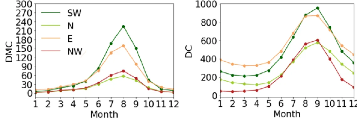
In the case of DMC and DC (Figure 4.2), as in the case of meteorological variables, two groups of regions can be highlighted. The SW and E regions stand out with higher mean values of DMC and DC when compared to N and NW values. Moreover, the highest DMC (DC) values occur in August (September) in all four regions.

Identification of Iberian large fires climate conditions

The choice of these four regions of the Iberian Peninsula confirms the distinct spatial-temporal clusters that characterize them in the first place (Trigo et al., 2013). In fact, it is possible to observe that the relative amount of burned area associated with each of the regions differs, as well as the peak time month, with the region E presenting its maximum of BA (Burned Area) in July, while in the N region that occurs in September and the SW and NW clusters, that include all the Portuguese territory, present a maximum in August.

4.2. Large fires classification

As described in the methodology, all events with burned areas above the 95th _{percentile of the}

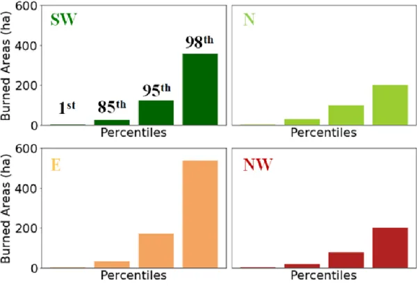
total distribution are considered as LF. Figure 4.4 shows the four histograms where the bars represent the 1st_{, 85}th_{, 95}th _{and 98}th _{percentile, respectively, for each of the described regions with the same colours}

used in Figure 2.1 (this approach will be followed in all the remaining figures). In addition to figure 4.4, and in order to facilitate analysis, the corresponding percentile values are shown in table 4.1. The analysis allows us to verify that the thresholds of the BA are quite different among the regions. The exception being the 1st _{percentile, since the BA are filtered to consider the fires with final burned areas}

higher than 1 ha, the 1st _{percentile is 1 ha for all regions. The 85}th _{percentile, although presenting}

different values for the four regions, is not drastically different among different regions. The E region presents the highest value (~32 ha), and the N region presents the lowest value (~20 ha). However, if

Figure 4.2 - As in Fig. 4.1 but for DMC and DC.

Figure 4.3 - Percentage of burned area during the months of May, June, July, August, September and October for the four regions.

Identification of Iberian large fires climate conditions

we consider the 95th _{percentile the threshold from which an LF is considered, the differences between}

regions are already considerable. The E region presents the highest burned area value of the four regions with 171 ha. The SW region is the one with the second highest threshold for an event to be considered an LF with about 125 ha there followed by the N region with 100 ha. Finally, the NW region is the one with the lowest threshold (~78 ha).

The very large fires (VLF) are characterised by having burnt area values above the 98th _percentile

thresh-old. Again, taking into account the results from Table 4.1, the E region is the one presenting the highest value of the burned area with 538 ha. In turn, the NW region has a threshold for which a VLF is consid-ered with 200 ha.

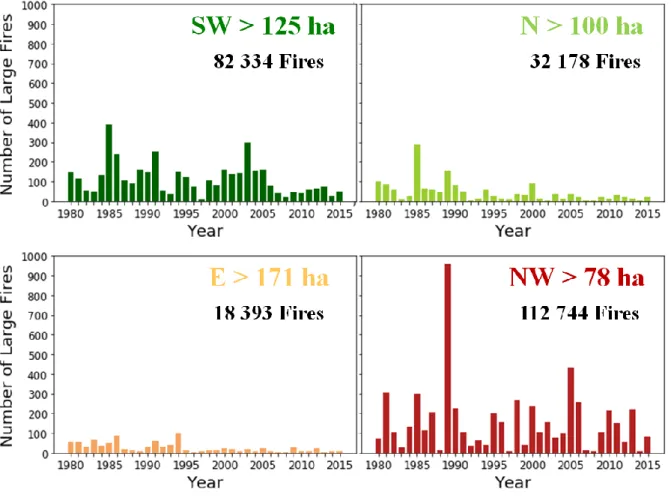
There is wide variability in the number of LF for the four regions of the IP (Figure 4.5). The NW region, although presenting the lowest LF threshold, is the one with the highest LF number and with the most fires (above 1 ha). The year of 1989 stands out with almost a thousand events. On the other hand, the E region, which presents the ultimate LF threshold of the four regions, is the one with the smallest LF number (below one hundred annual events).

Region 1st _{(ha) 85}th _{(ha) 95}th _{(ha) 98}th _(ha)

SW 1 25 125 357

N 1 30 100 202

E 1 32 171 538

NW 1 20 78 200

Figure 4.4 - Representation of the following representative percentiles: 1, 85, 95 and 98 for the four regions.

Identification of Iberian large fires climate conditions

4.3. Composite Analysis

4.3.1. Day of fire

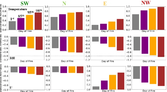
The standardized anomalies of the meteorological variables (temperature, relative humidity and zonal wind) for the day of the ignitions are recorded according to the percentile 1, 85, 95 and 98 of the total burned area for the four regions are represented in Figure 4.6. It is verified that for all regions, the anomalies of the meteorological variables increase in modulus according to the increase of the value of the total BA of the events. For the case of temperature, the standardized anomalies of the fire day are always positive and follow the behaviour already described, i.e., fires with a higher burned area are associated with days with higher temperature anomalies. In addition to this generalized behaviour, there are differences in the value of the anomalies when we compare results among the four considered re-gions. The NW region is the one that stands out with the highest anomalies of the meteorological varia-bles for all classes of burned areas. At the opposite extreme lies the E region, where fires occurring in this region exhibit the lowest temperature anomalies associated with fire days, although the distinction

Figure 4.5 - Interannual variability of the number of large fires per year observed in the four considered regions and the total number of all fires (> 1 ha).

Identification of Iberian large fires climate conditions

between all fires and large fires is visible. On the other hand, the SW and N regions have similar behav-iour in the case of the temperature anomalies for LF and the VLF, although, in the case of the N region, the difference between LF and VLF is not significant. When we consider all the fires indiscriminately, the N region stands out with the highest temperature anomalies (1st _percentile).

Relative humidity follows the opposite behaviour of temperature, as RH anomalies are increas-ingly negative for fires with higher burnt areas since its calculation depends directly on this variable.

Conversely, anomalies of zonal wind velocity present two very distinctive behaviours in the four regions, that accommodate the distinct signal (positive or negative) of zonal wind anomalies (U). Gen-erally speaking the SW, N and NW regions present negative zonal wind (U) anomalies on the fire days, with this relationship getting stronger with the fire size. For these three regions, the negative anomalies are indicative of prevailing winds from the eastern quadrant. Moreover, once again, the NW region presents anomalies, in this case of U, more intense when compared with the other regions, and the N region does not present significant differences between the U anomalies associated with the LF and the VLF. On the contrary, for the E region, the U anomalies grow positively with the increase of the burned area associated with an event. The positive sign of U anomalies is indicative of prevailing winds from the western quadrant.

A similar analysis was made for the FWI indices (Figure 4.7), displaying the standardized anom-alies of the indices of fuel dryness (DMC and DC). As in the case of the majority of the meteorological variables, DMC and DC present higher anomalies for higher burned areas. For the DMC, and contrary to the anomalies of the meteorological variables, it is the N region that presents the highest anomalies, and both, LF and VLF have DMC anomalies higher than one standard deviation. There is no difference between these two classes of burned areas and the same also occurs for the NW region, but with lower DMC anomaly values. Again, the E region is the one presenting the lowest anomalies when compared to the other regions, and it is possible to distinguish between the four classes of agreement of the final burned area, as in the SW region.

The magnitude of DC anomalies differs from the DMC anomalies. Both the NW and the N regions reveal the highest values of DC anomalies associated with the ignition days. In these two regions, there are variations in the value of DC anomalies for the four percentiles. Nevertheless, for the SW region, there are no differences in the anomalies between the four classes of burned areas.

Identification of Iberian large fires climate conditions

Figure 4.6 – Composites of standardized anomalies of temperature, relative humidity (RH) and zonal velocity of the wind (U) of the day of fire for the SW, N, E and NW regions according to the percentiles 1 (gray), 85 (purple), 95 orange), 98 (red) of the final burned areas.

Figure 4.7 – As in Fig. 4.6 but for DMC and DC.

Identification of Iberian large fires climate conditions

4.3.2. Twelve days

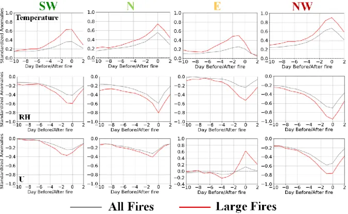
The daily standardized anomalies at a 12-day time scale (ten days before the start of the fire and two days after the beginning of the fire) of the temperature, relative humidity and zonal wind velocity are described on figure 4.8. With the representation of the composites for all the fires (grey) and the LF (red), it is intended to evaluate the influence of each of the meteorological variables on the activity of the fires and how the activity associated with the LF differs from the one associated to all fires activity. The zonal wind has a restricted influence on the day of the fire itself. In all cases, the anomalies decrease immediately after the fire day.

Looking at the SW region, it is possible to observe that both temperature and RH anomalies are higher (in absolute value) for the day of ignition and the previous day, particularly for LF. At the analyzed scale

(12 days), the difference in the distribution of the value of the anomalies for both variables for all fires and LF starts approximately six days before the fire day. The same temporal scale (six days) of signifi-cant separation between all fires and LF occurs in the E region, although it has lower anomalies than in the SW region. For the NW region, there is a much-hampered difference between the anomalies for all the fires and the LF than in the SW region. Subsequently, there is a significant increase in the value of the anomalies of temperature and RH, in the case of large fires, with only two days in advance of fire day. Finally, in the N region, although temperature and RH anomalies are always higher in the case of LF, the difference between the anomalies for both classes is constant.

For the indices representing the dryness of the fuels at different layers of the soil (Figure 4.9), it is observed that although the anomalies associated with the LF are always higher (except at SW region), the DMC as the DC does not have significant variations on a scale of 12 days. This behaviour was already expected since the DMC acts to evaluate a dryness of the fuels at 7 cm of depth and the DC at

Figure 4.8 - Composites of standardized anomalies of temperature, relative humidity and zonal wind velocity at 12 days for all fires (gray) and for large fires (red) for regions under study.

Identification of Iberian large fires climate conditions

18 cm of depth, and these indices do not, therefore, reflect the meteorological variations of the day, presenting a temporal lag.

4.3.3. Five Weeks

On a five-weeks scale (four weeks before fire and one week later) the standardized weekly tem-perature, relative humidity and zonal wind velocity anomalies show diverse anomalies for the different regions (Figure 4.10). The temperature has higher weekly anomalies for the fire week with anomalies ranging from 0.2 to 0.6 standard deviation (std) for LF in the four regions. In the SW, N and E regions, in both temperature and relative humidity, there is an increase in the weekly LF anomalies than those associated with all fires one week before the week of the event. For the NW region, although the anom-alies associated with the LF are always higher, there is no clear separation of the distribution of the weekly anomalies (temperature and relative humidity) of the LF and all the fires. Regarding the wind speed, there are no significant variations of the zonal component of the wind on this scale, except for the NW region, where the highest anomalies occur for both all fires and LF (LF reaches a maximum wind anomaly of 0.6 std).

Considering the previous analysis of the 12-day scale for the meteorological variables (section 4.3.2), the non-significance of the results at a 5-weeks scale was already expected, since the influence of the wind is limited to the day of the fire itself. Regarding temperature (and relative humidity) the anomalies are also in line with the results of the previous section with the weekly anomalies for the significant LF for the previous week or for the fire week itself.

The standardized weekly anomalies of the DMC and the DC (Figure 4.11) show that for the four regions considered the LF are associated with positive and higher anomalies of these two indices than when considering all fires. There is, however, an exception for the SW region when considering DC, in which case both fire classes have equal anomalies following the same behaviour of 12 days timescale.

However, this five-weeks time scale does not seem to be the most appropriate as a distinctive factor for the dryness of fuels between the two classes considered. Although the anomalies associated

Identification of Iberian large fires climate conditions

with the LF are higher, in particular in the N region for the DMC, the slopes of the anomaly curves are the same for the two classes, and it is not possible to determine for this time scale from which moment the anomalies associated with the LF distanced themselves from the other fires.

Figure 4.11 - As in Fig. 4.10 but for DMC and DC.

Figure 4.10 - Composites of standardized anomalies of temperature, relative humidity and zonal wind velocity at 5 weeks for all fires (gray) and for large fires (red) for the regions.

Figure 4.11 - As in Fig. 4.10 but for DMC and DC.Figure 4.10 - Composites of standardized anomalies of temperature, relative humidity and zonal wind velocity at 5 weeks for all fires (gray) and for large fires (red) for the regions.

Identification of Iberian large fires climate conditions

4.3.4. Eight months

At a timescale of 8 months, the standardized monthly anomalies of the meteorological variables are shown in Figure 4.12. For the case of the temperature, it is possible to verify that the monthly anomalies are always below 0.4 std for all the regions and for the two classes in the analysis (all the fires and the LF), where it is emphasized that the highest values occur during the fire season. The anomalies range from negative to positive between one and three months before the fire season considered, depending on the region. For relative humidity, the behaviour is analogous, but with negative anomalies, as previously described in this study. The anomalies on the monthly zonal wind velocity scale remain close to zero for both classes, with a slight peak during the fire season. When analysing the eight months composites, the anomalies decrease immediately after the fire season similarly to what was seen in the other temporal scales. Contrariwise to what happens in the remaining timescales, on the eight months timescale it is difficult to differentiate between the behaviour of LF and all the fires that occur for each one of these four regions.

Similarly to the previous timescales, the DMC and the DC composites were calculated for a time scale of 8 months (Figure 4.13). This longer time scale is appropriate to infer the dryness, not only of the fuels at different depths but also of the soil dryness itself, since both variables have as input the precipitation and the temperature, functioning as proxies of the drought and indicative of the pre-season fire conditions.

DMC and DC present rather different behaviour for this time scale. Although with different levels of standardized anomalies, two to three months before the fire season, the DMC anomalies for the LF generally start to rise, a month before the same escalation starts to become evident for the all fires curve.

Figure 4.12 - Composites of the monthly standardized anomalies for eight months temperature, relative humidity and zonal wind velocity for all fires (gray) and for large fires (red).

Identification of Iberian large fires climate conditions

Moreover, for the N and E regions, there is a clear difference in the distribution between all the fires and the LF from two months before the fire season. Finally, for the NW region, monthly DMC anomalies are practically identical.

The monthly distributions of the DC anomalies of all fires and the LF are not coincident, except for the SW region, and these become positive roughly two months before the fire season. In the N and SW regions, until two months before the fires, the distribution of the monthly anomalies associated with the LF is always below the anomalies where all the fires are included, which could be associated to the fact that the fire season being less dry. Only afterwards there is a reversal of this pattern and, in the previous month to the fire event, the registered DC anomalies for LF are considerably higher than for all fires.

4.4. Principal Component Analysis

. In order to quantify the importance of each of the meteorological variables and the indices that are representative of the dryness of the fuels to the LF activity on the ignition day, a Principal Component Analysis (PCA) was applied to each of the four regions of Iberia.

The explained variance attributed to each principal component is represented in figure 4.14, assigning a different colour in accordance to the meteorological variables depicted: temperature (red), relative humidity (green), zonal wind (blue), DMC (black), DC (pink) and precipitation (yellow), respectively, for the Southwest (SW), North (N), East (E) and Northwest (NW) regions.

For all regions, the variable with higher variance explained for the day of the fire, and thus the variable which dominates the activity associated with the LF is temperature. However, the amount of explained variability expressed by the temperature for each region is different. Temperature is followed

Identification of Iberian large fires climate conditions

Taking into account these results, and in order to reduce the dimensionality of the problem before applying the clusters analysis to each of the regions, it was decided to retain the first three principal components. These components represent the temperature, relative humidity and zonal wind speed, and explain more than 80% of the explained variance of all regions and thus, should be sufficient to identify the various groups of meteorological conditions (FWT) for the LF days. Therefore, the standardized anomalies associated with the days of ignition of temperature, RH and zonal wind velocity were used for each region before applying the K-Means algorithm.

4.5. K – Means Analysis: Fire Weather Types identification

Before applying the K-means algorithm, it was necessary to estimate the optimal number of clus-ters for each of the regions. To achieve this, the gap statistic method was applied, and three clusclus-ters were obtained for all regions.

The application of the cluster analysis to aggregate fire day standardized anomalies for the varia-bles identified by the PCA can be observed in figure 4.15, showing that in all four regions, three distinct

Figure 4.14 – Explained variance for the six principal components (PC 1 through PC 6) corresponding to the temperature (red), relative humidity (green), wind direction (blue), DMC (black), DC (pink) and precipitation (yellow) for the four regions of Iberia. The dashed blue line symbolizes the cumulative explained variance.

Figure 4.16 - As in Fig. 4.15 but for DMC and DC.Figure 4.14 – Explained variance for the six principal components (PC 1 through PC 6) corresponding to the temperature (red), relative humidity (green), wind direction (blue), DMC (black), DC (pink) and precipitation (yellow) for the four regions of Iberia. The dashed blue line symbolizes the cumulative explained variance.