Multivariate Copula-based SUR Tobit Models: A Modified Inference Function for Margins and Interval Estimation

(1)

Models: A Modified Inference Function for

Margins and Interval Estimation

Paulo Henrique Ferreira da Silva

Advisor: Prof. Dr. Francisco Louzada Neto

(2)

Models: A Modified Inference Function for

Margins and Interval Estimation

Paulo Henrique Ferreira da Silva

Advisor: Prof. Dr. Francisco Louzada Neto

Thesis submitted to Department of Statistics at Federal University of S˜ao Carlos for the award of degree of Doctor of Philosophy.

(3)

Ficha catalográfica elaborada pelo DePT da Biblioteca Comunitária/UFSCar

S586mc

Silva, Paulo Henrique Ferreira da.

Multivariate Copula-based SUR Tobit Models : a modified inference function for margins and interval estimation / Paulo Henrique Ferreira da Silva. -- São Carlos : UFSCar, 2015. 154 f.

Tese (Doutorado) -- Universidade Federal de São Carlos, 2015.

1. Probabilidades. 2. Intervalos de confiança. 3. Bootstrap

(Estatística). 4. Cópula. 5. Ampliação de dados. 6. Método de inferência para marginais modificado. I. Título.

(4)

(5)

Acknowledgements

I would like to express my special appreciation and thanks to my advisor Prof. Dr. Francisco Louzada Neto, for encouraging my research and for allowing me to grow as a research scientist. Your advice on both research as well as on my career have been invaluable.

I take this opportunity to express gratitude to all of the members of the Department of Statistics at Federal University of S˜ao Carlos, for their help and support.

A special thanks to my lovely parents, Alzira and Paulo S´ergio. Words can not express how grateful I am to you for all of the sacrifices that you have made on my behalf. I would also like to thank to my fianc´ee, Ana Paula, for her love, patience and ongoing faith on me.

(6)

Abstract

(7)

Resumo

Nesta tese de doutorado, consideramos os chamados modelos SUR (da expressão Seem-ingly Unrelated Regression) Tobit multivariados e estendemos a análise de tais modelos ao empregar fun¸cões de cópula para modelar estruturas com dependência não linear. As cópulas, dentre outras caracter´ısticas, possuem a importante habilidade (vantagem) de capturar/modelar a dependência na(s) cauda(s) do modelo SUR Tobit em que alguns dados são censurados (por exemplo, em análise econométrica, ensaios cl´ınicos e em ampla gama de fenômenos pol´ıticos e sociais, dentre outros, os dados são geralmente censurados à esquerda no ponto zero, ou à direita em um ponto d > 0 qualquer). Neste trabalho, propomos uma versão modificada do método clássico da Inferência para as Marginais (IFM, da expressão Inference Function for Margins), originalmente proposto por Joe & Xu (1996), a qual chamamos de MIFM, para estima¸cão (pontual) dos parâmetros do modelo SUR Tobit multivariado baseado em cópula. Mais especificamente, empregamos uma técnica (frequentista) de amplia¸cão de dados no segundo estágio do método IFM (o primeiro estágio do método MIFM é igual ao primeiro estágio do método IFM) para gerar as observa¸cões censuradas e, então, estimamos o parâmetro de dependência da cópula. Repetimos tal procedimento (amplia¸cão de dados e estima¸cão do parâmetro da cópula) até obter convergência. As razões para esta modifica¸cão no segundo estágio do método usual, são as seguintes: primeiro, construir/obter distribui¸cões marginais cont´ınuas, atendendo, então, ao teorema de unicidade da cópula resultante de Sklar (Sklar, 1959); e segundo, fornecer uma estimativa não viesada para o parâmetro da cópula (uma vez que o método IFM produz estimativas viesadas do parâmetro da cópula na presen¸ca de observa¸cões censuradas nas marginais). Tendo em vista a dificuldade adicional em calcular/obter a matriz de covariâncias assintótica das estimativas dos parâmetros, também propomos o uso de procedimentos de reamostragem (métodos bootstrap, tais como normal padrão e percentil, propostos por Efron & Tibshirani (1993), e básico, proposto por Davison

(8)

(9)

List of Figures

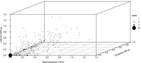
1.1 Distributions of the salad dressing (left panel), tomato (middle panel) and lettuce (right panel) consumption. The vertical line at zero on x axis repre-sents individuals that did not consume salad dressings, tomatoes or lettuce during the survey period. . . 5 1.2 3D scatter plot of salad dressing versus tomato versus lettuce. The bold

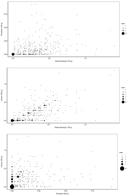
ball sizes are related to the number of pair of data with the same dependent variable values. . . 6 1.3 2D scatter plots of salad dressing versus tomato (upper panel), salad

dress-ing versus lettuce (middle panel) and tomato versus lettuce (lower panel). The bold ball sizes are related to the number of pair of data with the same dependent variable values. . . 12 1.4 Distributions of the log(time) to churn Product A (left panel), log(time) to

churn Product B (middle panel) and log(time) to churn Product C (right panel) variables. The vertical line at 2.3 on x axis represents customers still with the bank at the acquisition date. . . 13 1.5 3D scatter plot of log(time) to churn Product A versus log(time) to churn

Product B versus log(time) to churn Product C. The bold ball sizes are related to the number of pair of data with the same dependent variable values. . . 13 1.6 2D scatter plots of log(time) to churn Product A versus log(time) to churn

Product B (upper panel), log(time) to churn Product A versus log(time) to churn Product C (middle panel), and log(time) to churn Product B versus log(time) to churn Product C (lower panel). The bold ball sizes are related to the number of pair of data with the same dependent variable values. . . 14

(12)

2.1 Bias and MSE of the MIFM estimate of the Clayton copula parameter versus sample size, percentage of censoring in the margins and degree of dependence between them (normal marginal errors). . . 28 2.2 Bias and MSE of the MIFM estimate of the Clayton copula parameter

versus sample size, percentage of censoring in the margins and degree of dependence between them (power-normal marginal errors). . . 29 2.3 Bias and MSE of the MIFM estimate of the Clayton copula parameter

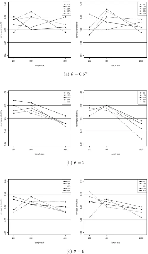
versus sample size, percentage of censoring in the margins and degree of dependence between them (logistic marginal errors). . . 30 2.4 Coverage probabilities (CPs) of the 90% standard normal (panels on the

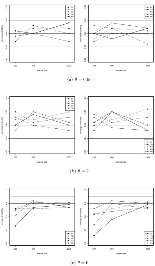
left) and percentile (panels on the right) confidence intervals for the Clayton copula parameter versus sample size, percentage of censoring in the margins and degree of dependence between them (normal marginal errors). The horizontal line at CP = 0.90 and the two horizontal lines at CP = 0.85 and 0.95 correspond, respectively, to the lower and upper bounds of the 90% confidence interval of the CP = 0.90. Thus, if a confidence interval has exact coverage of 0.90, roughly 90% of the observed coverages should be between these lines. . . 31 2.5 Coverage probabilities (CPs) of the 90% standard normal (panels on the

(13)

2.6 Coverage probabilities (CPs) of the 90% standard normal (panels on the left) and percentile (panels on the right) confidence intervals for the Clayton copula parameter versus sample size, percentage of censoring in the margins and degree of dependence between them (logistic marginal errors). The horizontal line at CP = 0.90 and the two horizontal lines at CP = 0.85 and 0.95 correspond, respectively, to the lower and upper bounds of the 90% confidence interval of the CP = 0.90. Thus, if a confidence interval has exact coverage of 0.90, roughly 90% of the observed coverages should be between these lines. . . 33 2.7 Comparison between the IFM and MIFM estimates of the Clayton copula

parameter, for n = 2000 (normal marginal errors). The averages of the parameter estimates are shown with a star symbol. The dotted horizontal line represents the true value of the Clayton copula parameter. . . 34 2.8 Comparison between the IFM and MIFM estimates of the Clayton copula

parameter, for n = 2000 (power-normal marginal errors). The averages of the parameter estimates are shown with a star symbol. The dotted horizontal line represents the true value of the Clayton copula parameter. 35 2.9 Comparison between the IFM and MIFM estimates of the Clayton copula

parameter, for n = 2000 (logistic marginal errors). The averages of the parameter estimates are shown with a star symbol. The dotted horizontal line represents the true value of the Clayton copula parameter. . . 36 2.10 Bias and MSE of the MIFM estimate of the Clayton survival copula

param-eter versus sample size, percentage of censoring in the margins and degree of dependence between them (normal marginal errors). . . 53 2.11 Bias and MSE of the MIFM estimate of the Clayton survival copula

param-eter versus sample size, percentage of censoring in the margins and degree of dependence between them (power-normal marginal errors). . . 54 2.12 Bias and MSE of the MIFM estimate of the Clayton survival copula

(14)

2.13 Coverage probabilities (CPs) of the 90% standard normal (panels on the left) and percentile (panels on the right) confidence intervals for the Clayton survival copula parameter versus sample size, percentage of censoring in the margins and degree of dependence between them (normal marginal errors). The horizontal line at CP = 0.90 and the two horizontal lines at CP = 0.85 and 0.95 correspond, respectively, to the lower and upper bounds of the 90% confidence interval of the CP = 0.90. Thus, if a confidence interval has exact coverage of 0.90, roughly 90% of the observed coverages should be between these lines. . . 56 2.14 Coverage probabilities (CPs) of the 90% standard normal (panels on the

left) and percentile (panels on the right) confidence intervals for the Clayton survival copula parameter versus sample size, percentage of censoring in the margins and degree of dependence between them (power-normal marginal errors). The horizontal line at CP = 0.90 and the two horizontal lines at CP = 0.85 and 0.95 correspond, respectively, to the lower and upper bounds of the 90% confidence interval of the CP = 0.90. Thus, if a confidence interval has exact coverage of 0.90, roughly 90% of the observed coverages should be between these lines. . . 57 2.15 Coverage probabilities (CPs) of the 90% standard normal (panels on the

left) and percentile (panels on the right) confidence intervals for the Clayton survival copula parameter versus sample size, percentage of censoring in the margins and degree of dependence between them (logistic marginal errors). The horizontal line at CP = 0.90 and the two horizontal lines at CP = 0.85 and 0.95 correspond, respectively, to the lower and upper bounds of the 90% confidence interval of the CP = 0.90. Thus, if a confidence interval has exact coverage of 0.90, roughly 90% of the observed coverages should be between these lines. . . 58 2.16 Comparison between the IFM and MIFM estimates of the Clayton survival

(15)

2.17 Comparison between the IFM and MIFM estimates of the Clayton survival copula parameter, forn = 2000 (power-normal marginal errors). The aver-ages of the parameter estimates are shown with a star symbol. The dotted horizontal line represents the true value of the Clayton survival copula parameter. . . 60 2.18 Comparison between the IFM and MIFM estimates of the Clayton survival

copula parameter, for n = 2000 (logistic marginal errors). The averages of the parameter estimates are shown with a star symbol. The dotted horizontal line represents the true value of the Clayton survival copula parameter. . . 61

3.1 Bias and MSE of the MIFM estimate of the Clayton copula parameter versus sample size, percentage of censoring in the margins and degree of dependence among them (normal marginal errors). . . 79 3.2 Bias and MSE of the MIFM estimate of the Clayton copula parameter

versus sample size, percentage of censoring in the margins and degree of dependence among them (power-normal marginal errors). . . 80 3.3 Bias and MSE of the MIFM estimate of the Clayton copula parameter

versus sample size, percentage of censoring in the margins and degree of dependence among them (logistic marginal errors). . . 81 3.4 Coverage probabilities (CPs) of the 90% standard normal (panels on the

(16)

3.5 Coverage probabilities (CPs) of the 90% standard normal (panels on the left), percentile (middle panels) and basic (panels on the right) confidence intervals for the Clayton copula parameter versus sample size, percentage of censoring in the margins and degree of dependence among them (power-normal marginal errors). The horizontal line at CP = 0.90 and the two horizontal lines at CP = 0.85 and 0.95 correspond, respectively, to the lower and upper bounds of the 90% confidence interval of the CP = 0.90. Thus, if a confidence interval has exact coverage of 0.90, roughly 90% of the observed coverages should be between these lines. . . 83 3.6 Coverage probabilities (CPs) of the 90% standard normal (panels on the

left), percentile (middle panels) and basic (panels on the right) confidence intervals for the Clayton copula parameter versus sample size, percentage of censoring in the margins and degree of dependence among them (logistic marginal errors). The horizontal line at CP = 0.90 and the two horizontal lines at CP = 0.85 and 0.95 correspond, respectively, to the lower and upper bounds of the 90% confidence interval of the CP = 0.90. Thus, if a confidence interval has exact coverage of 0.90, roughly 90% of the observed coverages should be between these lines. . . 84 3.7 Comparison between the IFM and MIFM estimates of the Clayton copula

parameter, for n = 2000 (normal marginal errors). The averages of the parameter estimates are shown with a star symbol. The dotted horizontal line represents the true value of the Clayton copula parameter. . . 85 3.8 Comparison between the IFM and MIFM estimates of the Clayton copula

parameter, for n = 2000 (power-normal marginal errors). The averages of the parameter estimates are shown with a star symbol. The dotted horizontal line represents the true value of the Clayton copula parameter. 86 3.9 Comparison between the IFM and MIFM estimates of the Clayton copula

(17)

3.10 Bias and MSE of the MIFM estimate of the Clayton survival copula param-eter versus sample size, percentage of censoring in the margins and degree of dependence among them (normal marginal errors). . . 104 3.11 Bias and MSE of the MIFM estimate of the Clayton survival copula

param-eter versus sample size, percentage of censoring in the margins and degree of dependence among them (power-normal marginal errors). . . 105 3.12 Bias and MSE of the MIFM estimate of the Clayton survival copula

param-eter versus sample size, percentage of censoring in the margins and degree of dependence among them (logistic marginal errors). . . 106 3.13 Coverage probabilities (CPs) of the 90% standard normal (panels on the

left), percentile (middle panels) and basic (panels on the right) confidence intervals for the Clayton survival copula parameter versus sample size, percentage of censoring in the margins and degree of dependence among them (normal marginal errors). The horizontal line at CP = 0.90 and the two horizontal lines at CP = 0.85 and 0.95 correspond, respectively, to the lower and upper bounds of the 90% confidence interval of the CP = 0.90. Thus, if a confidence interval has exact coverage of 0.90, roughly 90% of the observed coverages should be between these lines. . . 107 3.14 Coverage probabilities (CPs) of the 90% standard normal (panels on the

(18)

3.15 Coverage probabilities (CPs) of the 90% standard normal (panels on the left), percentile (middle panels) and basic (panels on the right) confidence intervals for the Clayton survival copula parameter versus sample size, percentage of censoring in the margins and degree of dependence among them (logistic marginal errors). The horizontal line at CP = 0.90 and the two horizontal lines at CP = 0.85 and 0.95 correspond, respectively, to the lower and upper bounds of the 90% confidence interval of the CP = 0.90. Thus, if a confidence interval has exact coverage of 0.90, roughly 90% of the observed coverages should be between these lines. . . 109 3.16 Comparison between the IFM and MIFM estimates of the Clayton survival

copula parameter, for n = 2000 (normal marginal errors). The averages of the parameter estimates are shown with a star symbol. The dotted horizontal line represents the true value of the Clayton survival copula parameter. . . 110 3.17 Comparison between the IFM and MIFM estimates of the Clayton survival

copula parameter, forn = 2000 (power-normal marginal errors). The aver-ages of the parameter estimates are shown with a star symbol. The dotted horizontal line represents the true value of the Clayton survival copula parameter. . . 111 3.18 Comparison between the IFM and MIFM estimates of the Clayton survival

(19)

List of Tables

1.1 Variable definitions and sample statistics (n= 400). . . 4 1.2 Variable definitions and sample statistics (n= 927). . . 5

2.1 Estimation results of bivariate Clayton copula-based SUR Tobit model with normal marginal errors for salad dressing and lettuce consumption in the U.S. in 1994-1996. . . 38 2.2 Estimation results of bivariate Clayton copula-based SUR Tobit model with

power-normal marginal errors for salad dressing and lettuce consumption in the U.S. in 1994-1996. . . 39 2.3 Estimation results of bivariate Clayton copula-based SUR Tobit model with

logistic marginal errors for salad dressing and lettuce consumption in the U.S. in 1994-1996. . . 40 2.4 Estimation results of basic bivariate SUR Tobit model with logistic marginal

errors for salad dressing and lettuce consumption in the U.S. in 1994-1996. 42 2.5 Estimation results of bivariate Clayton survival copula-based SUR Tobit

right-censored model with normal marginal errors for the customer churn data (Products A and B). . . 63 2.6 Estimation results of bivariate Clayton survival copula-based SUR Tobit

right-censored model with power-normal marginal errors for the customer churn data (Products A and B). . . 63 2.7 Estimation results of bivariate Clayton survival copula-based SUR Tobit

right-censored model with logistic marginal errors for the customer churn data (Products A and B). . . 64 2.8 Estimation results of basic bivariate SUR Tobit right-censored model for

the customer churn data (Products A and B). . . 64

(20)

3.1 Estimation results of trivariate Clayton copula-based SUR Tobit model with normal marginal errors for salad dressing, tomato and lettuce con-sumption in the U.S. in 1994-1996. . . 89 3.2 Estimation results of trivariate Clayton copula-based SUR Tobit model

with power-normal marginal errors for salad dressing, tomato and lettuce consumption in the U.S. in 1994-1996. . . 90 3.3 Estimation results of trivariate Clayton copula-based SUR Tobit model

with logistic marginal errors for salad dressing, tomato and lettuce con-sumption in the U.S. in 1994-1996. . . 91 3.4 Estimation results of basic trivariate SUR Tobit model with logistic marginal

errors for salad dressing, tomato and lettuce consumption in the U.S. in 1994-1996. . . 93 3.5 Estimation results of trivariate Clayton survival copula-based SUR Tobit

right-censored model with normal marginal errors for the customer churn data. . . 114 3.6 Estimation results of trivariate Clayton survival copula-based SUR Tobit

right-censored model with power-normal marginal errors for the customer churn data. . . 114 3.7 Estimation results of trivariate Clayton survival copula-based SUR Tobit

right-censored model with logistic marginal errors for the customer churn data. . . 115 3.8 Estimation results of basic trivariate SUR Tobit right-censored model for

(21)

Chapter 1 Introduction

The Tobit model refers to a class of regression models whose range of the dependent variable (or response variable) is somehow constrained. It was first proposed in 1958 by the 1981 Nobel Prize winner in Economic Sciences, James Tobin, to describe the relationship between a non-negative dependent variabley(the ratio of total durable goods expenditure to total disposable income, per household) and a vector of independent variables x (the age of the household head, and the ratio of liquid asset holdings to total disposable income) (see Tobin, 1958). Tobin called his model thelimited dependent variable model. However, it and its various generalizations are popularly known among economists asTobit models, a phrase coined by Goldberger (1964) because of similarities to probit models (the term Tobit aims to synthesize in one word the concept “Tobin’s probit”). Tobit models are also known ascensored ortruncated regression models.

Particularly, the presence of censoring (left-censoring, right-censoring or both) occurs when data on the dependent variable is limited or lost. Examples are:

1. Left-censoring. Antibody concentration values in Haitian 12-month-old infants vaccinated against measles are determined through neutralization antibody assays with the lower detection limit of 0.1 IU (Moulton & Halsey, 1995). Thus, concen-tration values under or equal to 0.1 are reported as 0.1.

2. Right-censoring. People of all income levels are included in the sample, but for some reason high-income people have their income coded as R$ 100,000 (Bolfarine, Santos, Correia, Mart´ınez, Gom´ez & Baz´an, 2013).

3. Both left- and right-censoring. Scores of students on an academic aptitude test can be any value between 200 and 800, and it is not rare to observe students

(22)

answering all questions in the test correctly, thus receiving a score of 800 (even though it is likely that these students are not “truly” equal in aptitude); or students answering all of the questions incorrectly, thus receiving a score of 200 (although they may not all be of equal aptitude).

The Tobit specification is appropriate for the situation in which the sample proportion of censored observations is roughly equivalent to the remaining tail area of the assumed parametric distribution. The Cragg (1971) model, which in the classical literature is known as the two-part model, is an alternative to Tobit when the data rate below or above the threshold is quite different from the probability of the tail obtained with the assumed parametric model.

The censoring problem also arises in situations with the presence of multiple dependent variables. For example, Chen & Zhou (2011) consider the joint problem of censoring and simultaneity when working with multivariate microeconomic data.

The next section describes two real datasets that show such characteristics (i.e. cen-soring and multiple correlated dependent variables).

1.1 The data

This section introduces the datasets that will be used to illustrate the approaches proposed in this thesis.

1.1.1 U.S. salad dressing, tomato and lettuce consumption data

(23)

eat large amounts of tomatoes, lettuce and other vegetables are curtailing consumption of salad dressings perceived as high in fat, calories and sodium.

Our study aims at establishing some factors (age, region/location and income, among others) that influence the consumption of tomatoes (including raw and cooked tomatoes, tomato juices, tomato sauces and mixtures having tomatoes as a main ingredient), lettuce (including all plain, Boston and Romaine lettuce reported separately or as part of a mixed salad or sandwich) and salad dressing products (including mayonnaise-type salad dressing reported separately or as part of a sandwich, and pourable salad dressings reported sep-arately or as part of a mixture such as a salad) by U.S. individuals. This study is based on part of a dataset extracted from the 1994-1996 Continuing Survey of Food Intakes by Individuals (CSFII) (USDA, 2000). In the CSFII, two non-consecutive days of dietary data for individuals of all ages residing in the United States were collected through in-person interviews using 24-hour recall. Each sample in-person reported the amount of each food item consumed. Where two days were reported there is also a third record contain-ing daily averages. Socioeconomic and demographic data for the sample households and their members were also collected in the CSFII. The size of the extracted sample here is

n= 400 adults age 20 or older. We only consider one member per household.

Table 1.1 provides the definitions and sample statistics for all considered variables, where we observe the proportions of consuming individuals in the dataset to range from 85.00% for salad dressings, to 63.25% for tomatoes and 67.25% for lettuce. Among those consuming, an individual on average consumes 32.84 g of salad dressings, 66.56 g of tomatoes and 60.52 g of lettuce per day.

(24)

Table 1.1: Variable definitions and sample statistics (n= 400).

Variable Definition Mean Standard

Deviation Dependent variables: amount consumed

Salad dressing (in 100 g) Quantity of salad dressings consumed 0.2791 0.2371

Among the consuming (n= 340; 85.00%) 0.3284 0.2235

Tomato (in 400 g) Quantity of tomatoes consumed 0.1052 0.1526

Lettuce (in 200 g) Quantity of lettuce consumed 0.2035 0.2348

Continuous explanatory variable

Income Household income as the proportion of 2.3160 0.8404

poverty threshold

Binary explanatory variables (yes = 1; no = 0)

Age 20-30 Age is 20-30 0.1375

Age 31-40 Age is 31-40 0.1600

Age 41-50 Age is 41-50 0.1900

Age 51-60 Age is 51-60 0.1725

Age>60 Age>60 (reference) 0.3400

Northeast Resides in the Northeastern states 0.1850

Midwest Resides in the Midwestern states 0.2450

South Resides in the Southern states (reference) 0.3500

West Resides in the Western states 0.2200

Source: Compiled from the CSFII, USDA, 1994-1996.

the reported salad dressing, tomato and lettuce consumption could be modeled through a trivariate regression model with limited (left-censored at zero) dependent variables.

1.1.2 Brazilian commercial bank customer churn data

Customer churn, also known as customer attrition or customer defection, has become a major issue for most banks in terms of representing the loss of clients or customers as they stop using certain products or services. According to Wang, Liu, Peng, Nie, Kou & Shi (2010), an important reason for customer churn analysis is that the cost of acquiring/developing a new customer is much higher than that of retaining an existing one. Generally, it costs up to five times as much to make a new sale to a new customer as it does to make an additional sale to an existing customer (Dixon, 1999; Slater & Narver, 2000). Reichheld & Sasser (1990) found that a bank can increase its profits by 85% by enhancing the customer retention rate by 5%.

(25)

Quantity (100 g)

Frequency

0.0 0.5 1.0 1.5

0

20

40

60

80

●

Quantity (400 g)

Frequency

0.0 0.2 0.4 0.6 0.8 1.0

0

50

100

150 ●

Quantity (200 g)

Frequency

0.0 0.5 1.0 1.5

0

20

40

60

80

100

120

140

●

Figure 1.1: Distributions of the salad dressing (left panel), tomato (middle panel) and lettuce (right panel) consumption. The vertical line at zero on x axis represents individuals that did not consume salad dressings, tomatoes or lettuce during the survey period.

Table 1.2: Variable definitions and sample statistics (n= 927).

Variable Definition Mean Standard

Deviation Dependent variables: in log of years

Product A Log of time to churn Product A 1.1200 0.9118

Among the uncensored (n= 777; 83.82%) 0.8925 0.8192

Product B Log of time to churn Product B 1.2610 0.8325

Product C Log of time to churn Product C 1.1500 0.8987

Continuous explanatory variable

Age Age in completed years 43.2000 15.0241

Income Monthly income in Brazilian reais (BRL) 1,524.0000 2,385.3710

acquisition (M&A) or takeover (Hildebrandt, 2007). Thus, the range of each dependent variable (time to churn Product A, time to churn Product B and time to churn Product C) is bounded by the interval zero year (i.e. customers close their accounts before completing the first year of the relationship) to ten years (i.e. customers still with the bank at the acquisition date).

Table 1.2 provides the definitions and sample statistics for all considered variables, where we observe the proportions of uncensored observations (i.e. customers whose log of time to churn is less than 2.3 or 10 years) in the dataset to range from 83.82% for Product A, to 80.37% for Product B and 82.52% for Product C. Among those uncensored, a customer on average churns Product A in 0.8925 log of years or 2.44 years; Product B in 1.0070 log of years or 2.74 years; and Product C in 0.9069 log of years or 2.48 years.

(26)

0.0 0.2 0.4 0.6 0.8 1.0 1.2 1.4 0.0 0.2 0.4 0.6 0.8 1.0 1.2 1.4 0.0 0.2 0.4 0.6 0.8 1.0

Salad dressings (100 g)

Lettuce (200 g)

Tomatoes (400 g)

● ●● ● ● ● ● ● ● ● ● ● ● ● ● ● ● ● ● ● ●●● ● ● ● ● ● ● ● ● ● ● ● ● ● ● ● ● ● ● ● ● ● ● ● ● ● ●● ● ● ● ● ● ● ●●● ● ● ● ● ● ● ● ● ● ● ● ● ● ● ● ● ● ● ● ● ● ● ● ● ● ● ● ● ● ● ● ● ● ● ● ● ● ● ● ● ● ● ● ● ● ● ● ● ● ● ● ● ● ● ● ● ● ● ●● ● ● ● ● ●● ● ● ● ● ● ● ● ● ● ● ● ● ● ● ● ● ● ● ● ● ● ● ● ● ● ● ● ● ● ● ● ● ● ● ● ● ● ● ● ● ● ● ● ● ● ● ● ● ● ● ● ● ● ● ● ● ● ● ● ● ● ● ● ● ● ● ● ● ● ● ● ● ● ● ● ● ● ● ● ● ● ● ● ● ● ● ●●● ● ● ● ● ● ● ● ● ● ● ● ● ● ● ● ● ● ● ● ● ● ● ● ● ● ● ● ● ● ● ● ● ● ● ● ● ● ● ● ● ● ● ● ● ● ● ● ● ● ● ● ● ● ● ● ● ● ● ● ● ● ● ● ● ● ● ● ● ● ● ● ● ● ● ● ● ● ● ● ● ● ● ● ● ● ● ● ● ● ● ● ● ● ● ● ● ● ● ● ● ● ● ● ● ● ● ● ● ● ● ● ● ● ● ● ● ● ● ● ● ● 1 2 3 60 count

Figure 1.2: 3D scatter plot of salad dressing versus tomato versus lettuce. The bold ball sizes are related to the number of pair of data with the same dependent variable values.

or approximately 10 years) and there is a considerable positive association among the log of times to churn Products A, B and C (the Kendall tau rank correlation coefficient between the log of times to churn Products A and B, Products A and C, and Products B and C is 0.6386, 0.5389 and 0.5928, respectively). These features, as well as the presence of covariates (age and income), suggest that the relationship among the reported log of times to churn Products A, B and C could be modeled through a trivariate regression model with limited (right-censored at pointd= 2.3) dependent variables.

1.2 Literature review

(27)

since the error terms are assumed to be correlated across the equations. See, e.g., Zell-ner (1962), Greene (2003, Chapter 14), Davidson & MacKinnon (2003, Chapter 12) and Zellner & Ando (2010) for more details on the SUR models; and Amemiya (1984) for a thorough review of various types of Tobit models.

Several estimation techniques have been proposed to implement the SUR Tobit model. See, e.g., Wales & Woodland (1983), Brown & Lankford (1992) and Kamakura & Wedel (2001) for the maximum likelihood (ML) estimation; Huang, Sloan & Adamache (1987) for the expectation-maximization; Meng & Rubin (1996) for the expectation-conditional maximization (ECM); and Huang (1999) for the Monte Carlo ECM (MCECM). Moreover, Huang (2001), Baranchuk & Chib (2008) and Taylor & Phaneuf (2009) implement the SUR Tobit model through the Bayesian approach using Gibbs samplers, while Chen & Zhou (2011) estimate the model parameters in the semiparametric context. However, all these estimation methods are cumbersome (i.e. computationally demanding and difficult to implement), especially for high dimensions. Trivedi & Zimmer (2005) suggest this as a reason why the SUR Tobit model is not well applied. These methods also assume nor-mal marginal error distributions, which may be inappropriate in many real applications. In addition, modeling the dependence structure of the SUR Tobit model through the multivariate normal distribution is restricted to the linear relationship among marginal distributions through the correlation coefficients.

(28)

U.S. out-of-pocket and non-out-of-pocket medical expenses data, finding that the two-stage ML/Inference Function for Margins (IFM) estimation results are unstable. This is not surprising considering the previous findings about the inconsistency of ML estima-tors of the parameters of the Tobit model with non-normal errors (Cameron & Trivedi, 2005). Yen & Lin (2008) estimate the copula-based censored equation system (a system of four meat products - beef, pork, poultry and fish - consumed by U.S. individuals) via the quasi-ML estimation method, yet considering the Frank copula with generalized log-Burr margins (the generalized log-log-Burr distribution nests the logistic distribution, which is kin to the normal distribution) exclusively. Finally, Wichitaksorn et al. (2012) apply and combine the data augmentation techniques by Geweke (1991), Chib (1992), Chib & Greenberg (1998), Pitt et al. (2006) and Smith & Khaled (2012) to simulate the unob-served marginal dependent variables and proceed with the bivariate copula-based SUR Tobit model implementation through Bayesian Markov Chain Monte Carlo methods as in other copula models with continuous margins. In their work, the relationship between the self-reported out-of-pocket and non-out-of-pocket medical expenses of elderly Amer-icans, as well as the relationship between the wage earnings income of household head and members living in the rural households in Thailand, are described by bivariate SUR Tobit models with Student-t margins through four different copulas (Gaussian, Student-t, Frank and Clayton).

1.3 Objectives

(29)

(30)

variables could be modeled through the bivariate SUR Tobit model with right-censored (at point d= 2.3) normally-, power-normally- or logistically-distributed dependent variables based on the Clayton survival copula. In this work, we also decided for the Clayton and Clayton survival copulas guided by the literature, which states that these copula families have a remarkable and useful (as will be seen in Sections 2.1.1.1, 2.2.1.1, 3.1.1.1, 3.2.1.1, 4.1.1.1 and 4.2.1.1) invariance property under truncation.

In short, the MIFM method proposed in this thesis uses a (frequentist) data aug-mentation technique at the second stage of the IFM method (the IFM method provides biased estimates of the Clayton and Clayton survival copulas’ association parameter, as will be seen in Sections 2.1.2.2, 2.2.2.2, 3.1.2.2 and 3.2.2.2) to generate the censored obser-vations/margins and thus obtain a better (unbiased) estimate of the copula dependence parameter. This modification also aims to satisfy the Sklar’s theorem, which states that marginal distributions should be continuous to ensure the uniqueness of the resulting cop-ula. Since the usual asymptotic approximation, that is the computation of the asymptotic covariance matrix of the parameter estimates, is cumbersome in this case, we consider re-sampling procedures (a parametric rere-sampling plan) to obtain confidence intervals for the copula-based SUR Tobit model parameters. More specifically, we use the standard normal and percentile methods by Efron & Tibshirani (1993), and the basic method by Davison & Hinkley (1997), to build bootstrap confidence intervals.

1.4 Overview

(31)

thesis for the m-variate (m ≥2) case. Finally, Chapter 5 concludes the thesis with final remarks and a few indications for further studies.

(32)

● ●● ● ● ● ● ● ● ● ● ● ● ● ● ● ● ● ● ● ●● ● ● ● ● ● ● ● ● ● ● ● ● ● ● ● ● ● ● ● ● ● ● ● ● ● ● ● ● ● ● ● ● ● ● ● ● ●● ● ● ● ● ● ● ● ● ● ● ● ● ● ● ● ● ●● ● ● ● ● ● ● ● ● ● ● ● ● ● ● ● ● ● ● ● ● ● ● ● ● ● ● ● ● ● ● ● ● ●● ● ●● ● ● ● ● ● ● ● ● ● ●● ● ● ● ● ● ●● ● ● ● ● ● ● ● ● ● ● ● ● ● ● ● ●● ● ● ● ● ● ● ● ● ● ●●● ● ● ● ● ●● ● ● ● ● ● ● ● ● ● ● ● ● ● ● ● ● ●●● ● ● ● ● ● ● ● ● ● ● ● ● ● ● ● ● ● ● ● ● ● ● ● ● ● ● ● ● ● ● ● ● ● ● ● ● ● ● ● ● ● ● ● ●● ● ● ● ● ● ● ● ● ● ● ● ● ● ● ● ● ● ● ● ● ● ● ● ● ● ● ● ● ● ● ● ● ● ● ● ● ● ● ● ● ● ● ● ● ● ● ● ● ● ● ● ● ● ● ● ● ● ● ● ● ● ● ● ● ● ● ● ● ● ● ● ● ● ● ● ● ● ● ● ● ● ● ● ● ● ● ● ● ● ● ● ● ● 0.00 0.25 0.50 0.75

0.0 0.5 1.0

T

omatoes (400 g)

count ● ● ● 1 2 3 60 ● ●● ● ● ●●● ● ● ● ● ● ●● ● ●●● ● ● ● ● ●● ● ● ● ● ● ● ● ● ● ● ● ● ● ● ● ● ● ● ● ● ● ● ● ● ● ● ●● ● ● ● ● ● ● ● ● ● ● ● ● ● ● ● ● ● ● ● ● ● ● ● ● ● ● ● ● ● ● ● ● ● ● ● ● ● ● ● ● ● ● ● ● ●● ● ● ● ● ● ● ● ● ● ● ● ● ● ● ● ● ● ● ● ● ● ● ● ● ● ●● ● ● ● ● ● ● ● ● ● ● ● ● ● ● ● ● ● ● ● ● ● ● ● ● ● ● ● ● ● ● ● ● ● ● ● ● ● ● ● ● ● ● ● ● ● ● ● ● ● ● ● ● ● ● ● ● ● ● ● ● ● ● ● ● ● ● ● ● ● ● ● ● ● ● ● ● ● ● ● ● ● ● ● ● ● ● ●● ● ● ● ● ● ● ● ● ● ● ● ● ● ● ● ● ● ● ● ● ● ●● ● ● ● ●● ● ● ● ● ● ● ● ● ● ● ● ● ● ● ● ● ● ● ● ● ● ● ● ● ● ● ● ● ● ● ● ● ● ● ● ● ● ● ● ● ● ● ● ● ● ● ● ● ● ● ● ● ● ● ● 0.0 0.5 1.0

0.0 0.5 1.0

Lettuce (200 g)

count ● ● ● ● ● 1 2 3 4 5 60 ● ● ● ● ● ● ● ● ● ● ● ● ● ● ● ● ● ● ● ● ● ● ● ● ● ● ●●● ● ● ● ● ● ● ● ● ● ● ● ● ● ● ● ● ● ● ● ● ● ● ● ● ● ● ● ● ● ● ● ● ● ● ● ● ●● ● ● ● ● ● ● ● ● ● ● ● ● ● ● ● ● ● ● ● ● ● ● ● ● ● ● ● ● ● ● ● ● ● ● ● ● ● ● ● ● ● ● ● ● ● ● ● ● ● ● ● ●● ● ● ● ● ● ● ● ● ● ● ● ● ● ● ● ● ● ●● ● ● ● ● ● ● ● ● ● ● ● ● ● ● ● ● ● ● ● ● ● ● ● ● ● ● ● ● ● ● ● ● ● ● ● ● ● ● ● ● ● ● ● ● ● ● ● ● ● ● ● ● ● ● ● ● ● ● ● ● ● ● ● ● ● ● ● ● ● ● ● ● ● ● ● ● ● ● ● ● ● ● ●● ● ● ● ● ● ● ●●● ● ● ● ● ● ● ● ● ● ● ● ● ● ● ● ● ● ● ● ●● ● ● ● ● ● ● ● ● ● ● ● ● ● 0.0 0.5 1.0

0.00 0.25 0.50 0.75

Tomatoes (400 g)

Lettuce (200 g)

count ● ● ● ● ● 1 2 3 5 7 99

(33)

log(time) to churn Product A

Frequency

−2 −1 0 1 2

0 50 100 150 200 ●

log(time) to churn Product B

Frequency

−1.0 −0.5 0.0 0.5 1.0 1.5 2.0

0 50 100 150 200 ●

log(time) to churn Product C

Frequency

−1 0 1 2

0 50 100 150 200 ●

Figure 1.4: Distributions of the log(time) to churn Product A (left panel), log(time) to churn Product B (middle panel) and log(time) to churn Product C (right panel) variables. The vertical line at 2.3 on x axis represents customers still with the bank at the acquisition date.

−3 −2 −1 0 1 2 3

−2 −1 0 1 2 3 −2 −1 0 1 2 3

log(time) to chur

n Product C

log(time) to chur n Product B

● ● ● ● ● ● ● ● ● ● ● ● ● ● ● ● ● ● ● ● ● ● ● ● ● ● ● ● ● ● ● ● ● ● ● ● ● ● ● ● ● ● ● ● ● ● ● ● ● ● ● ● ● ● ● ● ● ● ● ● ● ● ● ● ● ● ● ● ● ● ● ● ● ● ● ● ● ●● ● ● ● ● ● ● ● ● ● ● ● ● ● ● ● ● ● ● ● ● ● ● ● ● ● ● ● ● ● ● ● ● ● ● ● ● ● ● ● ● ● ● ● ● ● ● ● ● ● ● ● ● ● ● ● ● ● ● ● ● ● ● ● ● ● ● ● ● ● ● ● ● ● ● ● ● ● ● ● ● ● ● ● ● ● ● ● ● ● ● ● ● ● ● ● ● ● ● ● ● ● ● ● ● ● ● ● ● ● ● ● ● ● ● ● ● ● ● ● ● ● ● ● ● ● ● ● ● ● ● ● ● ● ● ● ● ● ● ●● ● ● ● ● ● ● ● ● ● ● ● ● ● ● ● ● ● ● ● ● ● ● ● ● ● ● ● ● ● ● ● ● ● ● ● ● ● ● ● ● ● ● ● ● ● ● ● ● ● ● ● ● ● ● ● ● ● ● ● ● ● ● ● ● ● ● ● ● ● ● ● ● ●● ● ● ● ● ● ● ● ● ● ● ● ● ● ● ● ● ● ● ● ● ● ● ● ● ● ● ● ● ● ● ● ● ● ● ● ● ● ● ● ● ● ● ● ● ● ● ● ● ● ● ● ● ● ● ● ● ● ● ● ● ● ● ● ● ● ● ● ● ● ● ● ● ● ● ● ● ● ● ● ● ● ● ● ● ● ● ● ● ● ● ● ● ● ● ● ● ● ● ● ● ● ● ● ● ● ● ● ● ● ● ● ● ● ●● ● ● ●● ● ● ● ● ● ● ● ● ● ● ● ● ● ● ● ● ● ● ● ● ● ● ● ● ● ● ● ● ● ● ● ● ● ● ● ● ● ● ● ● ● ● ● ● ● ● ● ● ● ● ● ● ● ● ● ● ● ● ● ● ● ● ● ● ● ● ● ● ● ● ● ● ● ● ● ● ● ● ● ● ● ● ● ● ● ● ● ● ● ● ● ● ● ● ● ● ● ● ● ● ● ● ● ● ● ● ● ● ● ● ● ● ● ● ● ● ● ● ● ● ● ● ● ● ● ● ● ● ● ● ● ● ● ● ● ● ● ● ● ● ● ● ● ● ● ● ● ● ● ● ● ● ● ● ● ● ● ● ● ● ● ● ● ● ● ● ● ● ● ● ● ● ● ● ● ● ● ● ● ● ● ● ● ● ● ● ● ● ● ● ● ● ● ● ● ● ● ● ● ● ● ●● ● ● ● ● ● ● ● ● ● ● ● ● ● ● ● ● ● ● ● ● ● ● ● ● ● ● ● ● ● ● ● ● ● ● ● ● ● ● ● ● ● ●● ● ● ● ● ● ● ● ● ● ● ● ● ● ● ● ● ● ●● ● ● ● ● ● ● ● ● ● ● ● ● ● ● ● ●● ● ● ● ● ● ● ● ● ● ● ● ● ● ● ● ● ● ● ● ● ● ● ● ● ● ● ● ● ● ● ● ● ● ● ● ● ● ● ● ● ● ● ● ● ● ● ●● ● ● ● ● ● ●●●● ● ● ● ● ● ● ● ● ● ● ● ● ● ● ● ● ● ● ●● ● ●● ● ● ● ● ● ● ● ● ● ● ● ● ● ● ● ● ● ● ● ● ● ● ● ● ● ● ● ●● ● ● ● ● ● ● ● ● ● ● ● ● ● ● ● ● ● ● ● ● ●●●● ● ● ● ● ● ● 1 95 count

(34)

● ● ● ● ● ● ● ● ● ● ● ● ● ● ● ● ● ● ● ● ● ● ● ● ● ● ● ● ● ● ● ● ● ● ● ● ● ● ● ● ● ● ● ● ● ● ● ● ● ●● ● ● ● ● ● ● ● ● ● ● ● ● ● ● ● ● ● ● ● ● ● ● ● ● ● ● ● ● ● ● ● ● ● ● ● ● ● ● ● ● ● ● ● ● ● ● ● ● ● ● ● ● ● ● ● ● ● ● ● ● ● ● ● ● ● ● ● ● ● ● ● ● ● ● ● ● ● ● ● ● ● ● ● ● ● ● ● ● ● ● ● ● ● ● ● ● ● ● ● ● ● ● ● ● ●● ● ● ● ● ● ● ● ● ● ● ● ● ● ● ● ● ● ● ● ● ● ● ● ● ● ● ● ● ● ● ● ● ● ● ● ● ● ● ● ● ● ● ● ● ● ● ● ● ● ● ● ● ● ● ● ● ● ● ● ● ● ● ● ● ● ● ● ● ● ● ● ● ● ● ● ● ● ● ● ● ● ● ● ● ● ● ● ● ● ● ● ● ● ● ● ● ● ● ● ● ● ● ● ● ● ● ● ● ● ● ● ● ● ● ● ● ● ● ● ● ● ● ● ● ● ● ● ● ● ● ● ● ● ● ● ● ● ● ● ● ● ● ● ● ● ● ● ● ● ● ● ● ● ● ● ● ● ● ● ● ● ● ● ● ● ● ● ● ● ● ● ● ● ● ● ● ● ● ● ● ● ● ● ● ● ● ● ● ● ● ● ● ● ● ● ● ● ● ● ● ● ● ● ● ● ● ● ● ● ● ● ● ● ● ● ● ● ● ● ● ● ● ● ● ● ● ● ● ● ● ● ● ● ● ● ● ● ● ● ● ● ● ● ● ● ● ● ● ● ● ● ● ● ● ● ● ● ● ● ● ● ● ● ● ● ● ● ● ● ● ● ● ● ● ● ● ● ● ● ● ● ● ● ● ● ● ● ● ● ● ● ● ● ● ● ● ● ● ● ● ● ● ● ● ● ● ● ● ● ● ● ● ● ● ● ● ● ● ● ● ● ● ● ● ● ● ● ● ● ● ● ● ● ● ● ● ● ● ● ● ● ● ● ● ● ● ● ● ● ● ● ● ● ● ● ● ● ● ● ● ● ● ● ● ● ● ● ● ● ● ● ● ● ● ● ● ● ● ● ● ● ● ● ● ● ● ● ● ● ● ● ● ● ● ● ● ● ● ● ● ● ● ● ● ● ● ● ● ● ● ● ● ● ● ● ● ● ● ● ● ● ● ● ● ● ● ● ● ● ● ● ● ● ● ● ● ● ● ● ● ● ● ● ● ● ● ● ● ● ● ● ● ● ● ● ● ● ● ● ● ● ● ● ● ● ● ● ● ● ● ● ● ● ● ● ● ● ● ● ● ● ● ● ● ● ● ● ● ● ● ● ● ● ● ● ● ● ● ● ●● ● ● ●● ● ● ● ● ● ● ● ● ● ● ● ● ● ● ● ● ● ● ● ● ● ● ● ● ● ● ● ● ● ● ● ● ● ● ● ● ● ● ● ●● ● ● ●● ● ● ● ● ● ● ● ● ● ● ● ● ● ● ● ●● ● ● ● ● ● ● ● ● ● ● ● ● ● ● ●● ● ● ● ● ● ● ● ●●●● ● ● ● ● ● ● ● ● ● ● ● ● ●● ● ● ● ● ● ● ● ● ● ● ● ● ● ● ● ● ● ● ● ● ● ● ● ● ● ● ● ● ● ● ● ● ● ● ● ● ● ● ● ● −1 0 1 2

−2 −1 0 1 2

log(time) to chur

n Product B

count ● 1 122 ● ● ● ● ● ● ● ● ● ● ● ● ● ● ● ● ● ● ● ● ● ● ● ● ● ● ● ● ● ● ● ● ● ● ● ● ● ● ● ● ● ● ● ● ● ● ● ● ● ● ● ● ● ● ● ● ● ● ● ● ● ● ● ● ● ● ● ● ● ● ● ● ● ● ● ● ● ● ● ● ● ● ● ● ● ● ● ● ● ● ● ● ● ● ● ● ● ● ● ● ● ● ● ● ● ● ● ● ● ● ● ● ● ● ● ● ● ● ● ● ● ●● ● ● ● ● ● ● ● ● ● ● ● ● ● ● ● ● ● ● ● ● ● ● ● ● ● ● ● ● ● ● ● ● ● ● ● ● ● ● ● ● ● ● ● ● ● ● ● ● ● ● ● ● ● ● ● ● ● ● ● ● ● ● ● ● ● ● ● ● ● ● ● ● ● ● ● ● ● ● ● ● ● ● ● ● ● ● ● ● ● ● ● ● ● ● ●● ● ● ● ● ● ● ● ● ● ● ● ● ● ● ● ● ● ● ● ● ● ● ● ● ● ● ● ● ● ● ● ● ● ● ● ● ● ● ● ● ● ● ● ● ● ● ● ● ● ● ● ● ● ● ● ● ● ● ● ● ● ● ● ● ● ● ● ● ● ● ● ● ● ● ● ● ● ● ● ● ● ● ● ● ● ● ● ● ● ● ● ● ● ● ● ● ● ● ● ● ● ● ● ● ● ● ● ● ● ● ● ● ● ● ● ● ● ● ● ● ● ● ● ● ● ● ● ● ● ● ● ● ● ● ● ● ● ● ● ● ● ● ● ● ● ● ● ● ● ● ● ● ● ● ● ● ● ● ● ● ● ● ● ● ● ● ● ● ● ● ● ● ● ● ●● ● ● ● ● ● ● ● ● ● ●● ● ● ● ● ● ● ● ● ● ● ● ● ● ● ● ● ● ● ● ● ● ● ● ● ● ● ● ●● ● ● ● ● ● ● ● ● ● ● ● ● ● ● ● ● ● ● ● ● ● ● ● ● ● ● ● ● ● ● ● ● ● ● ● ● ● ● ● ● ● ● ● ● ● ● ● ● ● ● ● ● ● ● ● ● ● ● ● ● ● ● ● ● ● ● ● ● ● ● ● ● ● ● ● ● ● ● ● ● ● ● ● ● ● ● ● ● ● ● ● ● ● ● ● ● ● ● ● ● ● ● ● ● ● ● ● ● ● ● ● ● ● ● ● ● ● ● ● ● ● ● ● ● ● ● ● ● ● ● ● ● ● ● ● ● ● ● ● ● ● ● ● ● ● ● ● ● ● ● ● ●● ● ● ● ● ● ● ● ● ● ● ● ● ● ● ● ● ● ● ● ● ● ● ● ● ● ●● ● ● ● ● ● ● ● ● ● ● ● ● ● ● ● ● ● ● ● ● ● ● ● ● ● ● ● ● ● ● ● ● ● ● ● ● ● ● ● ● ● ●● ● ● ●● ● ● ● ● ● ● ● ● ● ● ● ● ●●● ● ● ● ● ● ● ● ● ● ● ● ● ● ● ● ● ● ● ● ● ● ● ● ● ● ● ● ● ● ● ● ● ● ● ● ● ● ● ● ● ● ● ●● ● ● ● ● ● ● ● ● ● ● ● ● ● ● ● ● ● ● ●● ● ● ● ● ● ● ●●●● ● ● ● ● ● ● ●● ● ● ● ● ● ● ● ● ● ● ●● ● ● ● ● ● ● ● ● ● ● ● ● ● ● ● ● ● ● ● ● ● ● ● ● ● ● ● ● ● ● ● ● ● ● ● ● ● ● ● ● ● ● ● ● −1 0 1 2

−2 −1 0 1 2

log(time) to chur

n Product C

count ● 1 112 ● ● ●● ● ● ● ● ●● ● ● ● ● ● ● ● ● ● ● ● ● ● ● ● ● ● ● ● ● ● ● ● ● ● ● ● ● ● ● ● ● ● ● ● ● ● ● ● ● ● ● ● ● ● ● ● ● ● ● ● ● ● ● ● ● ● ● ● ● ● ● ● ● ● ● ● ●● ● ●● ● ● ● ● ● ● ●● ● ● ● ● ● ● ● ● ● ● ● ● ● ● ● ● ● ● ● ● ● ● ● ● ● ● ● ● ● ● ●● ● ● ● ● ● ● ● ● ● ● ● ● ● ● ● ● ● ● ● ● ● ● ● ● ● ● ● ● ● ● ● ● ● ●●● ● ● ● ● ● ● ● ● ● ● ● ● ● ● ● ● ● ● ● ● ● ● ● ● ● ● ● ● ● ● ● ● ● ● ● ● ● ● ● ● ● ● ● ● ● ● ● ● ● ● ● ● ● ● ● ● ● ●● ● ● ● ● ● ● ● ● ● ● ● ● ● ● ● ● ● ● ● ● ● ● ● ● ● ● ● ● ● ● ● ● ● ● ● ● ● ● ● ● ● ● ● ● ● ● ● ● ● ● ● ● ● ● ● ● ● ● ● ● ● ● ● ● ● ● ● ● ● ● ● ● ● ● ● ● ● ● ● ● ● ● ● ● ● ● ● ● ● ● ● ● ● ● ● ● ● ● ● ● ● ● ● ● ● ● ● ● ● ● ● ● ● ● ● ● ● ● ● ● ● ● ● ● ● ● ● ● ● ● ●● ● ● ● ● ● ● ● ● ● ● ● ● ● ● ● ● ● ● ● ● ● ● ● ● ● ● ● ● ●● ● ● ● ● ● ● ● ● ● ● ● ● ● ● ● ● ● ● ● ● ● ● ● ● ● ● ● ● ● ● ● ● ● ● ● ● ● ● ● ● ● ● ● ● ● ● ● ● ●● ● ● ● ● ● ● ● ● ● ● ● ● ● ● ● ● ● ● ● ● ● ● ● ● ● ● ● ● ● ● ● ●● ● ● ● ● ● ● ● ● ● ● ● ● ● ● ● ● ● ● ● ● ● ● ● ● ● ● ● ● ● ● ● ● ● ● ● ● ● ● ● ● ● ● ●● ● ● ● ● ● ● ● ● ● ● ● ● ● ● ● ● ● ● ● ● ● ● ● ● ● ● ● ● ● ● ● ● ● ● ● ● ● ● ● ● ● ● ● ● ● ● ● ● ●● ● ● ● ● ● ● ● ● ● ● ● ● ● ● ● ● ● ● ● ● ● ● ● ● ● ● ● ● ● ● ● ● ● ● ● ● ● ● ● ● ● ● ● ● ●● ● ● ● ● ● ● ● ● ● ● ● ● ● ● ● ● ● ● ● ● ● ● ● ● ● ● ● ● ● ● ● ● ● ● ● ● ● ● ●● ● ● ● ● ● ● ● ● ● ● ● ● ● ● ● ● ● ● ● ● ● ● ● ● ● ● ● ● ● ● ● ● ● ● ● ● ● ● ● ● ● ● ● ● ● ● ● ● ● ● ● ● ● ● ● ● ● ● ● ● ● ● ● ● ● ● ● ● ● ● ● ● ● ● ● ● ●●● ● ● ● ● ●● ● ● ● ● ● ● ● ● ● ● ● ●● ● ● ● ● ● ● ● ● ● ● ● ● ● ● ● ● ● ● ● ● ● ● ● ● ● ● ● ● ● ● ● ● ● ● ● ● ● ● ● ● ● ● ● ● ● ● ● ● ● ● ● ● ● ● ● ● ● ● −1 0 1 2

−1 0 1 2

log(time) to churn Product B

log(time) to chur

n Product C

count

● ₁

129

(35)

Chapter 2 Bivariate Copula-based SUR Tobit

Models

In this chapter, we present the bivariate copula-based SUR Tobit models proposed in this thesis. We first present the bivariate Clayton copula-based SUR Tobit model, i.e. the SUR Tobit model with two left-censored (at zero point) dependent variables whose dependence between them is modeled through the Clayton copula. Then, we present the bivariate Clayton survival copula-based SUR Tobit right-censored model, which is the SUR Tobit model with two right-censored (at pointdj >0, j = 1,2) dependent variables

whose dependence structure between them is modeled by the Clayton survival copula. In both cases, we assume symmetric, asymmetric and heavy-tailed distributions for the marginal error terms. Discussions concerning the model implementation through the pro-posed MIFM method, as well as the confidence intervals construction from the bootstrap distribution of model parameters, are made for each proposed model. Simulation studies and applications to real datasets are also provided in this chapter.

2.1 Bivariate Clayton copula-based SUR Tobit model

formulation

The SUR Tobit model with two left-censored (at zero point) dependent variables, or simply bivariate SUR Tobit model, is expressed as

y∗_ij =x′_ijβ_j +ǫij,

yij =

    

y∗

ij if yij∗ >0,

0 otherwise,

(36)

for i = 1, ..., n and j = 1,2, where n is the number of observations, y∗

ij is the latent (i.e.

unobserved) dependent variable of margin j, yij is the observed dependent variable of

marginj (which is defined to be equal to the latent dependent variable y∗

ij whenever yij∗

is above zero and zero otherwise), x_ij is the k ×1 vector of covariates, β_j is the k×1 vector of regression coefficients andǫij is the marginj’s error that follows some zero mean

distribution.

Suppose that the marginal errors are no longer normal, but they are assumed to be distributed according to the power-normal (Gupta & Gupta, 2008) and logistic models, thus providing asymmetric and heavy-tailed alternatives to Tobin’s model (Tobin, 1958). These choices of error distribution consist of expressing the density function of yij in the

following forms.

• Normal marginal errors (i.e. ǫij ∼N 0, σj2

):

fj yij|xij,βj, σj

=

      

1−Φ

x′_ijβj

σj

if yij = 0,

1

σjφ

yij−x′ijβj

σj

if yij >0,

(2.1)

(Trivedi & Zimmer, 2005), where φ(.) and Φ (.) are the standard normal probability density function (p.d.f.) and cumulative distribution function (c.d.f.), respectively. Note that if ǫij ∼N 0, σj2

, then we have marginal standard Tobit models or Type I Tobit models (Amemiya, 1984). The corresponding distribution function of yij

is denoted by Fj yij|xij,βj, σj and is obtained by replacing φ(.) with Φ (.) and

removing 1/ σj from the second part of (2.1) (i.e. where yij >0).

• Power-normal marginal errors (i.e. ǫij ∼P N(0, σj, αj)):

fj yij|xij,βj, σj, αj

=

      

Φ

−x

′

ijβj

σj

αj

if yij = 0,

αj

σjφ

yij−x

′

ijβj

σj Φ

yij−x

′

ijβj

σj

αj−1

if yij >0,

(2.2)

where αj > 0 is a shape parameter that controls the amount of asymmetry in

the distribution, as well as the distribution kurtosis (for αj > 1, the kurtosis is

greater than that of the normal distribution, and for 0 < αj < 1 the opposite

is observed). Note that (2.1) is recovered when αj = 1. For further details on

the power-normal distributions, see Gupta & Gupta (2008). If we assume ǫij ∼

(37)

Bolfarine & G´omez, 2013). The corresponding distribution function ofyij is denoted

by Fj yij|xij,βj, σj, αj

and is obtained by replacing φ(.) with Φ (.) and removing

αj/ σj from the second part of (2.2) (i.e. where yij >0).

• Logistic marginal errors (i.e. ǫij ∼L(0, sj)):

fj yij|xij,βj, sj=

      

1−G

x′_ijβ_j

sj

if yij = 0,

1

sjg

yij−x

′

ijβj

sj

if yij >0,

(2.3)

whereg(z) =ez_/_{(1 +}_ez₎2

andG(z) = 1/(1 +e−z_{) are the}_L₍₀_,_{1) p.d.f. and c.d.f.,}

respectively. The corresponding distribution function of yij, Fj yij|xij,βj, sj

, is obtained by replacing g(.) with G(.) and removing 1/ sj from the second part of

(2.3) (i.e. where yij >0).

Usually, the dependence between the error terms ǫi1 and ǫi2 is modeled through a

bi-variate distribution, especially the bibi-variate normal distribution (such specification char-acterizes the basic bivariate SUR Tobit model; see, e.g., Huang et al. (1987) for more details on this model). However, as commented before (in Section 1.2), a restriction in applying a bivariate distribution to the bivariate SUR Tobit model is the linear re-lationship between marginal distributions through the correlation coefficient. One way to overcome this restriction is to use a copula function to capture/model the nonlinear dependence structure in the bivariate SUR Tobit model.

Thus, for the censored outcomes yi1 and yi2, the bivariate copula-based SUR Tobit

distribution is given by

F (yi1, yi2) =C(ui1, ui2|θ),

where, e.g., uij = Fj yij|xij,βj, σj if ǫij ∼ N 0, σj2

, Fj yij|xij,βj, σj, αj if ǫij ∼

P N(0, σj, αj), andFj yij|xij,βj, sj

ifǫij ∼L(0, sj), forj = 1,2, andθis the association

parameter (or parameter vector) of the copula, which is assumed to be scalar.

SupposeC is the bidimensional Clayton (1978) copula, also referred to as the Cook & Johnson (1981) copula, originally studied by Kimeldorf & Sampson (1975). It takes the form

C(ui1, ui2|θ) = ui−1θ+u−i2θ−1

−1

θ _, _(2.4)

(38)

dependence. The Clayton copula does not allow for negative dependence. In the survival analysis framework, there is an equivalence between the Clayton copula and the shared gamma frailty model (see, e.g., Goethals, Janssen & Duchateau, 2008). Trivedi & Zimmer (2005) point out that the Clayton copula is widely used to study correlated risks because it shows strong left tail dependence and relatively weak right tail dependence. Indeed, when correlation between two events is stronger in the left tail of the joint distribution, Clayton is usually an appropriate modeling choice.

2.1.1 Inference

In this subsection, we discuss inference (point and interval estimation) for the parameters of the bivariate Clayton copula-based SUR Tobit model. Particularly, by considering/as-suming normal, power-normal and logistic distributions for the marginal errors.

2.1.1.1 Estimation through the MIFM method

According to Trivedi & Zimmer (2005), the log-likelihood function for the bivariate Clay-ton copula-based SUR Tobit model can be written in the following form1

ℓ(η) =

n

X

i=1

logc(F1(yi1|xi1,υ1), F2(yi2|xi2,υ2)|θ) +

n

X

i=1

2

X

j=1

logfj(yij|xij,υj), (2.5)

where η = (υ1,υ2, θ) is the vector of model parameters, υj is the marginj’s parameter

vector,fj(yij|xij,υj) is the p.d.f. ofyij,Fj(yij|xij,υj) is the c.d.f. ofyij, andc(ui1, ui2|θ),

with uij = Fj(yij|xij,υj), is the p.d.f. of the Clayton copula, which is calculated from

(2.4) as

c(ui1, ui2|θ) =

∂2_C₍_u

i1, ui2|θ) ∂ui1∂ui2

= (θ+ 1) (ui1ui2)−θ−1 u−i1θ+u−i2θ−1

−1

θ−2_.

For model estimation, the use of copula methods, as well as the log-likelihood function form given by (2.5), enables the use of the (classical) two-stage ML/IFM method by Joe & Xu (1996), which estimates the marginal parametersυ_j at a first step through

b

υj,IFM = arg max

υj

n

X

i=1

logfj(yij|xij,υj), (2.6)

forj = 1,2, and then estimates the association parameterθ given υb_j,_IFM by

b

θIFM = arg max

θ n

X

i=1

logc F1(yi1|xi1,υb1,IFM), F2(yi2|xi2,υb2,IFM)|θ

. (2.7)

(39)

Note that each maximization task (step) has a small number of parameters, which reduces the computational difficulty. However, the IFM method provides a biased estimate for the parameter θ in the presence of censored observations for both margins (as will be seen in Section 2.1.2.2). Since we are interested in the bivariate Clayton copula-based SUR Tobit model where both marginal distributions are censored/semi-continuous, we are dealing with the case where there is not a one-to-one relationship between the marginal distributions and the copula, i.e. there is more than one copula to join the marginal distributions. This constitutes a violation of the Sklar’s theorem (Sklar, 1959). When it occurs, researchers often face problems in the copula model fitting and validation.

In order to facilitate the implementation of copula models with semi-continuous mar-gins, the semi-continuous marginal distributions could be augmented to achieve continuity. More specifically, we can use a (frequentist) data augmentation technique to simulate the latent (i.e. unobserved) dependent variables in the censored margins, that is, we generate the unobserved data with all properties, e.g., mean, variance and dependence structure that match with the observed ones, and obtain the continuous marginal distributions (Wi-chitaksornet al., 2012). Thus, in order to obtain an unbiased estimate for the association parameter θ, we replace yij by the augmented data yija, or equivalently and more simply

(thus, preferred by us), we can replaceuij by the augmented uniform data uaij at the

sec-ond stage of the IFM method and proceed with the copula parameter estimation as usual for the continuous margin cases. This process (uniform data augmentation and copula parameter estimation) is then repeated until convergence occurs (MIFM method). The (frequentist) data augmentation technique we employ here is partially based on Algorithm A2 presented in Wichitaksorn et al.(2012). For alternative ways of implementing copula models with censored observations in the margins, but in a survival analysis framework, see, e.g., the classical work of Shih & Louis (1995), as well as its Bayesian counterpart developed by Romeo, Tanaka & Pedroso-de Lima (2006).

(40)

yi2 = 0, oryi1 = 0 and yi2 >0), the uniform data augmentation is performed through the

truncated conditional distribution of the Clayton copula. If the inverse conditional distri-bution of the copula used has a closed-form expression, which is the case of the Clayton copula (see, e.g., Armstrong, 2003), we can generate random numbers from its truncated version by applying the method by Devroye (1986, p. 38-39). Otherwise, numerical root-finding procedures are required. By observing the results in Oakes (2005), we see that the Clayton copula has a remarkable invariance property under truncation, such that the conditional distribution ofui1 andui2 in a sub-region of a Clayton copula, with one corner

at (0,0), can be written by means of a Clayton copula. That formulation enables a simple simulation scheme (see, e.g., the following online short note: http://web.cecs.pdx.edu/ ~cgshirl/Documents/Research/Copula_Methods/Clayton%20Copula.pdf) in the cases where both dependent variables/margins are censored (i.e. whenyi1 =yi2 = 0). For

cop-ulas that do not have the truncation-invariance property, an iterative simulation scheme could be used.

The implementation of the bivariate Clayton copula-based SUR Tobit model with arbitrary margins through the proposed MIFM method can be described as follows. In particular, if the marginal error distributions are normal, then set υj = βj, σj and

Hj(z|xij,υj) = Φ z−x

′

ijβj

/ σj

; if marginal error distributions are power-normal, so υj = βj, σj, αj and Hj(z|xij,υj) = Φ z−x

′

ijβj

/ σj αj

; and if marginal error distributions are logistic, then υ_j = β_j, sj

and Hj(z|xij,υj) = G z−x

′

ijβj

/ sj

=

1 + exp− z−x′_ijβ_j/ sj −

1

, for j = 1,2 and z ∈R.

Stage 1. Estimate the marginal parameters using (2.6). Set υˆj,MIFM = υˆj,IFM, for j = 1,2.

Stage 2. Estimate the copula parameter using e.g., (2.7). Set ˆθ(1)_MIFM = ˆθIFM and then

consider the algorithm below.

Forω = 1,2, ...,

Fori= 1,2, ..., n,

Ifyi1 =yi2 = 0, then draw (uai1, uai2) from C

ua

i1, uai2|θˆ

(ω)

MIFM

(41)

1. Draw (p, q) fromCp, q|θˆ(_MIFMω) =p−θˆ_MIFM(ω) ₊_q−θˆ_MIFM(ω) ₋₁−1/θˆ (ω) MIFM

. See, e.g., Arm-strong (2003) for the Clayton copula data generation.

2. Compute bij =Hj(0|xij,υˆj,MIFM), for j = 1,2.

3. Set ua

i1 =

b−θˆ

(ω) MIFM

i1 +b

−θˆ(_MIFMω)

i2 −1

p−θˆ_MIFM(ω) _{+ 1}₋_b−θˆ(MIFMω) i2

−1/θˆ(_MIFMω)

.

4. Set ua

i2 =

b−θˆ

(ω) MIFM

i1 +b

−θˆ(_MIFMω)

i2 −1

q−θˆ(_MIFMω) _{+ 1}₋_b−θˆMIFM(ω) i1

−1/θˆ(_MIFMω)

.

Ifyi1 = 0 andyi2 >0, then drawuai1fromC

ua

i1|ui2,θˆ(MIFMω)

truncated to the interval (0, bi1). This can be done according to the following steps.

1. Compute ui2 =H2(yi2|xi2,υˆ2,MIFM).

2. Compute bi1 =H1(0|xi1,υˆ1,MIFM).

3. Draw t fromU nif orm(0,1).

4. Compute vi1 =t

 

b−θˆ

(ω) MIFM

i1 +u

−θˆ_MIFM(ω)

i2 −1

−1/θˆ(_MIFMω) −1

u−θˆ

(ω)

MIFM−1

i2 .

5. Set ua

i1 =

v− ˆ

θ_MIFM(ω) /θˆ(_MIFMω) +1

i1 −1

u−θˆ

(ω) MIFM

i2 + 1

−1/θˆ(_MIFMω)

.

Ifyi1 >0 andyi2 = 0, then drawuai2fromC

ua

i2|ui1,θˆ(MIFMω)

truncated to the interval (0, bi2). This can be done by following the five steps of the previous case (i.e. yi1 = 0 and yi2 >0) by switching subscripts 1 and 2.

If yi1 > 0 and yi2 > 0, then set uai1 = ui1 = H1(yi1|xi1,υˆ1,MIFM) and uai2 = ui2 = H2(yi2|xi2,υˆ2,MIFM).

Given the generated/augmented marginal uniform dataua

ij, we estimate the association

parameterθ by2

ˆ

θ_MIFM(ω+1) = arg max

θ n

X

i=1

logc(ua_i₁, ua_i₂|θ).

The algorithm stops if a termination criterion is fulfilled, e.g. if |θˆ(_MIFMω+1) −θˆ_MIFM(ω) | < ξ, whereξ is the tolerance parameter (e.g.,ξ = 10−3_).

2_{The generated/augmented marginal uniform data} _ua

ij should carry (ω) as a superscript, i.e. u

a(ω)