Received: 25 May 2009 – Published in Hydrol. Earth Syst. Sci. Discuss.: 19 June 2009 Revised: 29 October 2009 – Accepted: 7 November 2009 – Published: 3 December 2009
Abstract. From the point of view of multisite stochastic daily rainfall modelling, there are two new ideas introduced in this paper. The first is the use of asymmetrical copulas to model the spatial interdependence structure of the rainfall amounts together with the rainfall occurrences in one rela-tionship. The second is in the evaluation of the (necessary but often ignored) congregating behaviour of the higher val-ues of simulated rainfall; this evaluation is performed by cal-culating the entropy of the observations at all the near equi-lateral triangles that can be formed from the sequences at the gauge sites, as a function of their mutual separation distance. It turns out that the model captures the qualities desired and offers a fresh approach to a relatively mature problem in hy-drometeorology.
1 Introduction
In 21st century hydrology, there is a growing need to match precipitation simulation to the fine spatial scale of distributed hydrological models. Random fields mimicking radar rain-fields offer an attractive possibility, but the lowly rain-gauge is still the instrument of choice for conditioning such fields. Without a good model for multi-site daily rainfall at gauge sites, a random field model would likely be missing some connection to the reality of the detail, particularly those as-pects dependent on location. It is the purpose of this paper to delve into the underlying interdependence between daily rain-gauge readings in a variable terrain and model it faith-fully.
Careful study of the dependence structure of many hy-drometeorological data sets, both spatial and temporal, re-veals that the dependence is more complex than that mod-elled by conventional correlation of the multivariate normal.
Correspondence to:A. B´ardossy ([email protected])
The tool used in this paper for modelling this complex de-pendence is the multivariate copula, relating observations at many sites in space and time. The advantages that can be as-cribed to using copula densities to represent interdependence between variables include the following properties:
– The empirical copulas (probability density scatterplots in many dimensions) are independent of their corre-sponding marginal distributions, so that copulas display interdependence between variables in its purest or es-sential form.
– Empirical copulas are easily computed from data. – Differences in types of association between variables
are readily identified by copula shape.
– A suite of theoretical copula density functions has been developed to model these attributes.
A careful examination of sample copulas of hydrometeo-rological processes reveals, however, that there is frequently a significant departure of the dependence structure from that of the bivariate Gaussian which is simply defined by its cor-relation coefficient. The question posed and answered in this paper is: How does one exploit this knowledge in simulation of multi-site daily rainfall?
1.1 Simulation of multi-site Time Series of daily precipitation
Srikanthan and McMahon (2001) gave an extensive review of rainfall models, including multisite network modelling. There has since been continued interest in the subject and we name some of the activity (this is not an exhaustive list as we use a different modelling procedure in this pa-per). Srikanthan (2005) generated the daily rainfall values via a season-dependent multisite AR(1) model, based on the work of Wilks (1998), which was then post-conditioned to give the observed monthly and annual variations. Mehro-tra et al. (2006) compared three multi-site stochastic weather generators, including (i) a parametric hidden Markov model (HMM), (ii) the Srikanthan (2005) multi-site stochastic pre-cipitation generation model proposed by Wilks (1998) and (iii) a non-parametric K-nearest neighbour (KNN) model, concluding that Wilks-based model had the edge. Apipat-tanavis et al. (2007) used a semiparametric blend of Markov chains and Bootstrap resampling. Mehrotra and Sharma (2007) proposed a modification of the traditional Markov chain approach for modelling the occurrences, using an ana-lytically derived factor that represents the influence of rain-fall aggregated over long time periods in an attempt to incor-porate low-frequency variability in simulation. Srikanthan and Pegram (2009) extended the post-conditioning in the ear-lier work of Srikanthan (2005) to include spatial as well as temporal dependence to the same end.
One of the notable features of rainfall estimated by radar is that the low frequency fluctuations of the random field are ev-ident in zones of higher rainfall distinct from zones of lower rainfall. Data sampled from raingauge networks also exhibits this behaviour (the grouping of high separate from low val-ues) but is not so obvious. This strong spatial dependence has its origins in the physics of rainfall accumulations and has traditionally been modelled by two-dimensional tools in the past (covariance and variogram functions, for example) and we suggest that the spatial interdependence is stronger than can be captured by pairwise modelling.
To model this spatial dependence we go part of the way to multidimensional copulas by introducing stronger depen-dence structures for high rainfall values than low ones. To test this congregating property by using bivariate correlations is not enough. To ascertain whether rainfall data and simula-tions can capture the higher dimensional spatial dependence structure, we have devised a spatial statistic based on the joint probabilities of rainfall behaviour, above certain thresholds,
measured at the vertices of nearly equilateral triangles over a range of sizes in the gauge network. The measure of associ-ation depends on the entropy of the 3-variate 2-state proba-bilities of each triangular set, defined by a quantile threshold of choice. We chose this configuration because acute angled triangles, in the limit, degenerate to straight lines, destroy-ing the spatial property we wish to explore. We choose to call this behaviour “congregating” rather than use the word “clustering” which has other connotations.
By congregation, we mean that on a particular day of rain on a region, the wet gauges will tend to group in a small num-ber of sub-regions, with the interior of each of the congrega-tions experiencing more rainfall than the edges fringed by dry gauges, as observed in the records. We suggest that the multisite copula-based model will dynamically model that feature better, because the wet-dry process and the amount process are jointly described by the dependencies captured by the multivariate copulas. This is the important innovation of the modelling procedure introduced herein.
Turning to the detail of jointly modelling occurrences and amounts of rainfall at more than one site, Herr and Krzyszto-fowicz (2005) developed a normal quantile based procedure for modelling pairs of rain gauge records, in particular they separately modelled the dry and wet probabilities and the marginal and joint wet distributions. In this paper, we use that approach as a point of departure to model many sites through the use of multivariate copulas which implicitly cap-ture the pair-wise joint wet and dry processes as well as the mixed wet and dry possibilities. The approach goes be-yond the combination of Markov chains for occurrences and the separate generation of correlated amounts for the wet sites used previously by most authors quoted above. These are typified by Srikanthan and Pegram (2009), who used a two-tiered model: a multi-site bivariate Markov chain to model the wet-dry occurrences and a multivariate Gamma AR(1) process to model the jointly wet events. Although that model satisfactorily mimics and reproduces the histor-ical daily, monthly and annual statistics, there is no feature built in to that approach to mimic the congregation of high values, other than cross-correlation.
The sites of the records studied in this paper appear in Fig. 1 in a region which has non-homogeneous meteoro-logical characteristics, effectively a mesoscale sized area in Baden-W¨urtemberg in South-West Germany. 32 stations with daily records from 1958 to 2001 were selected and are located around the Black Forest on the west and east side of the mountains, chosen particularly because of the hetero-geneity of the statistics of the records.
The resolution of the data is 0.1 mm, so that any ob-servation less than this threshold is taken to be a dry day. Examining such a record reveals intermittency of rainfall, in both space and time. From experience and observation, clouds produce highly variable precipitation in random con-gregations. These events range from intermittent, locally intense, and fragmentary convective ones, to long-lasting, well spread, persistent, stratiform ones. The statistics of the daily raingauge observations of the observed events reflect these characteristics, occurrences being isolated or congre-gated in space and time, while the amounts are relatively highly skewed.
The spatial dependence structure of daily rainfall is more complex than can be modelled by a simple correlation co-efficient over the range of observed values. Where the ob-served values are low, they tend to be scattered and inter-mittent, exhibiting a poor spatial dependency. By contrast, where the rainfalls are high, they tend to be spatially and temporally more dependent. This interdependence which is related to the amount of rain needs an appropriate technique to describe it. The choice here is the multivariate copula; only a short introduction on copulas is given here; readers interested in more general details are referred to Joe (1997), Nelsen (1999), or Salvadori et al. (2007).
A copula is defined as a distribution function on the n-dimensional unit cube. All marginal distributions are uni-form:
C:[0,1]n→[0,1] (1)
C (u)=ui if the vector u=(1,...,1,ui,1,...,1) (2)
For everyndimensional hypercube within the unit hyper-cube, the corresponding probability has to be non-negative. Copulas and multivariate distributions are linked to each
Fig. 1.The locations of the rain gauge stations indicated by circled dots, around the Black Forest within the German state of Baden-W¨urttemberg used in this study; shading darkens with increasing altitude above sea level. Stations 1 and 23 are coloured brown and blue respectively and will be used in the discussion in Section 2.2. The full numbering appears in Fig. 8.
other by Sklar’s theorem Sklar (1959). Sklar proved that each multivariate distributionF (t1,...,tn)can be represented with
the help of a copula:
F (t1,...,tn)=C Ft1(t1),...Ftn(tn)
(3) whereFti(ti) represents the i-th one-dimensional marginal
distribution of the multivariate distribution. If the distribu-tion is continuous then the copulaCis unique. Copulas can be constructed from distribution functions, as described by Nelsen (1999):
C (u)=C (u1,...,un)=F
Ft−1
1 (t1),...F −1
tn (tn)
(4) The advantage of using a copula is that it is invariant to strictly increasing monotonic transformations of the vari-ables. Thus the frequent dilemma whether to transform data or not (for example taking the natural logarithms) does not occur in this case.
An interesting and important property of a copula is whether the corresponding dependence is the same for high or low values. A bivariate copula expresses a symmetrical dependence if:
C (u,v)=C (1−u,1−v)−1+u+v (5)
which means that the copula density is symmetrical with re-spect to the secondary diagonalu=1−vof the unit square and the copula densitycsatisfies:
(a)
(b)
Fig. 2. Two sample copulas for station pairs 1 and 23, the upper panel(a)for Summer (June to August) and the bottom panel(b)for the relatively wetter Winter (December to February); see Fig. 10 for station locations and Table 1 forP[0] values in January and July, which are close to the thresholds in these figures.
2.2 Examples of empirical copulas of daily rainfall
Copulas are most usefully visualised as bivariate densities rather than bivariate cumulative functions of joint probabil-ity on the space[0,1]2. In Fig. 2 we show two examples of empirical copulas derived from scatter-plots of pairs of daily recording rain gauges. The empirical copula densities sam-pled from the pair of stations 1 and 23 (on opposite sides of the divide as will be seen in Fig. 1), appear in Fig. 2a and b, respectively for summer (June, July, and August) and for winter (December, January, and February). The horizon-tal and vertical lines indicate the probability limits for the dry/wet boundaries, both evidently drier in summer than in
winter. These figures exhibit a constant density for the “both dry” condition in the plateau defined in the lower left cor-ner. The upper left and lower right quadrants show the one-dimensional marginal densities of the wet gauge given that the other is dry, thus one can see all the conditional distribu-tions in one figure.
2.3 Examples of models of theoretical copulas for multisite rainfall
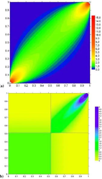
Figure 3a shows an example of the bivariate normal copula with a relatively high constant correlation of 0.85, which is seen to exhibit symmetry about both diagonals. We note that any Normal Quantile (scores) transform from arbitrary joint distribution functions to Gaussian, allowing the modelling of the correlation structure of the bivariate Normal to dictate the interdependence, will maintain the bisymmetric nature of the bivariate normal copula. Thus low values will be as well correlated as high values, as is expected in the normal copula. The image in Fig. 3b shows the partitioned version of the normal copula in Fig. 3a.
Evidently there is a need to model the observed depen-dence structure more carefully than via the normal score transform, whose dependence structure is locked into the bi-variate normal copula, independent of any monotonic quan-tile transform. This fundamental property (of the interdepen-dence between the variables being completely unaffected by the transformations of the field variables’ marginal distribu-tions) is not easy to grasp until it is fully understood that the dependence structure displayed by the copula is dependent only on the rank of the observation, not its marginal distribu-tion.
No monotonic transform of the normal distribution is go-ing to yield a copula in character different to Fig. 3. Theo-retical models of copulas are difficult to come by, however, B´ardossy (2006) introduced some which provide a basis for achieving the type of asymmetrical behaviour found in em-pirical copulas, of which Fig. 2 is an example.
(a)
(b)
Fig. 3. (a)Bivariate normal copula density withρ=0.85, the lower panel(b)is the partitioned version of the upper panel (a), where
P[zero rainfall]=0.51 in each case.
in Fig. 4a and in the copulas of data of Fig. 2a and b. The parameters will be defined in the theoretical development in the next section.
In contrast to the work of Serinaldi (2008) who concen-trated on the upper-tail dependence structure of 2-copulas, we are concerned about the joint interdependence of congre-gations of rainfall stations. Congregation behaviour is the feature of widespread flood-causing rainfall and it is this fea-ture which we do not want to lose in the rainfall model. We are particularly interested in the joint modelling of multisite daily rainfall and would eventually like to model the spatial behaviour, not as a conglomerate of bivariate relationships as has been done with the multinormal, but as jointly multidi-mensional copulas as was done by B´ardossy and Li (2008). However, the copula model we chose for this rainfall network
(a)
(b)
(c)
Fig. 4. Copula densities using the v- transform copula model with hidden normal density: (a) k=4.0, m=0, ρ=0.75, (b)
application is still a multisite bivariate model in principle, as it is predicated on a hidden covariance Gaussian model. To check if this copula-based model can capture spatial dependence better than the conventional covariance based model, we use the entropy of the observations of the trian-gular triples. This entropy procedure is fully developed in Sect. 3.4.
3 The model
3.1 Theory behind the model
The rainfall observed at sitei=1,2,...,non daytis labelled zi(t ). To model these data, we work through three stages: a
hidden multisite AR(1) time series model; a non-linear trans-form to an intermediate variable defining the copulas; the transform of the quantiles defined by the copulas to the sim-ulated field variables.
The multi-site Auto-Regressive lag-1, or AR(1) model, suggested by Pegram and James (1972), based on the seminal paper of Matalas (1967), is used as the driver for the multi-site rainfall model, for both the dry and wet occurrences and the wet amounts, specified as follows:
y(t ) = diag{ri(t )}y(t−1)+diag
n
1−ri2(t )1/2oa(t ) where:
y(t ) = {yi(t ),i=1,2,...,n}is a vector of correlated
Gaussian variates corresponding to each of the n sites on dayt, suitably transformed from thezi(t )observations.
ri(t ) = are the serial correlations between theyi-values
and depend on the month in whichtfalls; they have to be inferred after the transformation by the copula of thez-values to theys in the Gaussian domain
a(t ) = B(t )e(t )is a cross-correlated “noise” vector B(t ) is the “square root” matrix of the
cross-correla-tion matrixG(t )relating they(t )through thea(t )-values during the month corresponding to dayt, in the sense thatBTB
=G e(t ) is ann-vector of IID standardised
Gaussian random variates.
In this model the serial dependence is restricted to each site, while the cross-correlation comes through the noise term a(t ). The factorisation of Gis achieved by singular value decomposition (SVD) (see for example Press et al., 1992), which is stable even if Gis ill-conditioned. Briefly, SVD decomposesGintoG=V W UT, whereW is diagonal and comprises the singular values.UandV are orthonormal and in the particular case thatGis square (the case of a covari-ance matrix),UTV =I.Bmay be (not uniquely) computed asV W1/2UT, whereW1/2=diag{w1i/2}, so thatB=BT. In this formulationB is full, not triangular as in Cholesky decomposition which fails whenGis ill-conditioned.
The relationship between thehiddenyi(t )values and the
corresponding rainfall amountszi(t )(including the dry days)
is developed through the following transform; this relation-ship is used both for estimation and for simulation.
The transform for the copulas works as follows:yis Gaus-sian; we define an intermediate variables=g(y), where
g(y)=m−y if y < m
=k(y−m)α otherwise (7)
Note that ifm=0 andk=α=1, theng(y)= |y|, so in that case, the non-linear transformg(.)is based on a non-shifted modulus.
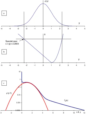
Figure 5 shows the relationship, form=1 andk=α=2 in three stages: the standard normal in the upper panel, then the transformation fromy tosin the middle panel and then in the lower panel, a comparison of the densities of the two distributions, the shifted normal and the V-copula-based one: φ (m−y)andfg(s). Note the long tail insin the case of the
latter.
Returning to the development, the distribution function of S=g(Y )is thus
Fg(s)=P[S < s]=Pm−s < Y < (s/ k)1/α+m
=8
(s/ k)1/α+m
−8[m−s] (8) and the density function ofSis
fg(s)=
1 kα
s k
1α−1 φ s k 1α +m
+φ[m−s] (9) shown in comparison with the normal densityφ (y−m), with m=1 in Fig. 5.
To picture the relationship, the points where s= |y| are computed and shown explicitly in the middle panel of Fig. 5: we getP[S <2.2808] =P[−2.2808< Y <2.2808], as shown by the intersections of the horizontal and vertical lines.
Whenm >3, then8[(s/ k)1/α+m] ≈1 thusFg(s)≈1−
8[m−s] =8[s−m], so that s approaches Gaussianity in this case.
The quantile defined by the cdfFg(s)is related to the
cor-responding rainfall amount through the transform: zi(t )=Fz−i1
Fg(s) (10)
whereFzi[.]is the marginal (mixed discrete and continuous)
cdf ofzi(t )at theith site, whose parameters are dependent
on the month into whichtfalls.
Fig. 5.The copula variablestransformed from the Gaussiany. The value ofsindicated by the horizontal line in the middle panel(b)of the figure is 2.2808. The vertical lines, through the intersection of thes=2.2808 line with thes=g(y)curves, are the two values ofy
definings, and in the upper panel(a)they bound the segment of the standard normal distribution integrated to giveP[S < s], leading to the cdfFg(s)of s. The densitiesφ (y−m)&fg(s)appear in the
lowest panel(c).
see that the blue distribution corresponding to the high non-linear transformed values on the right arm of the v-transform produces much higher precipitation values than the red distri-bution derived from the left arm, which is in fact a segment of the (untransformed) normal distribution. A special analysis (not detailed here) of the correlations within sets of precip-itation values generated from the two arms of the V-copula transform, shows that the correlation between the series is different for the two different generating mechanisms. For the above defined parameters with P[0]=0.5 one has a cor-relation of 0.81 for the precipitation amounts corresponding to the lower arm of the V-transformation and 0.48 for the upper arm. Thus the lower arm represents the advective (or stratiform) processes better than the upper arm, which corre-sponds to scattered occasionally very intense (or convective) precipitation.
Fig. 6.Division of rainfall amount distribution corresponding to the left arm of the transformation (advective/stratiform precipitation) – red line and to the right arm (convective precipitation) – blue line. Parameters used for this transformation arem=1.5,k=2,α=2, and a Weibull distribution of the precipitation amounts is assumed.
In more detail, we can extract the wet amount and dry in-formation directly fromsdepending on the dry probability at a siteion a given dayt:
zi(t )=0 if Fg(s)<pi(t ) =F−1
wi
Fg(s)−pi(t ) /{1−pi(t )}
otherwise (11)
Here Fwi(z) is the distribution function of precipitation
amounts at location ion wet days, pi(t )is the probability
of a dry day at locationi. The above definition leads to cor-rect marginals at each observation location.
The interdependence of precipitation amounts is obtained through the interdependence structure ofY. The main diffi-culty in this representation is that the parameters of the hid-denYandghave to be estimated by searching for the correct parameter set, whereZis the only observed information set; this has to be done by maximum likelihood using nonlinear optimisation.
The spatial dependence between precipitation observa-tions is described by the copula of the multivariate distri-bution defined by the transformation functiong(y)through the correlation matrix G of the hidden Gaussian variables y. Note that this copula C(u1,u2,...,un) is only properly
defined forui> pi(t ), because of the pole of probability at
(0,0)and in addition, the ‘conditional’ marginal distributions Fg(ui,0)andFg(0,uj)fori6=j, are spread over the left and
bottom quadrants of the copula, as shown in Fig. 2.
distribution of the y-variates. The distribution function is: Fg si,sj=PSi(t ) < si,Sj(t ) < sj=
=Pg (Yi) < si,g Yj< sj
=PhYi< (si/ k)1/α+m,Yj< sj/ k1/α
+mi−
PhYi< m−si,Yj< sj/ k1/α
+mi−
P
Yi< (si/ k)1/α+m,Yj< m−sj
+
P
Yi< m−si,Yj< m−sj
=82
h
(si/ k)1/α+m, sj/ k1/α
+m
i
−
82
h
m−si, sj/ k1/α+m
i
−
82(si/ k)1/α+m,m−sj+
82m−si,m−sj.
(12)
Here82 is the bivariate normal distribution function, with standard normal marginals and correlation ρ. The corre-sponding density required for finding the parameters of the hidden AR(1) model, for the case of two sites by maximum likelihood are found by differentiation:
∂2Fg si,sj
/∂si∂sj=fg si,sj
fg si,sj
= n
1/ k2α2 sisj/ k2 1/α−1o
φ2
h
(si/ k)1/α+m, sj/ k 1/α
+mi+ n
1/(kα) sj/ k 1/α−1o
φ2
h
m−si, sj/ k 1/α
+mi+
1/(kα)(si/ k)1/α−1 φ2
(si/ k)1/α+m,m−sj
+
φ2
m−si,m−sj
.
(13)
Then-dimensional joint density can be derived similarly and with largenthis soon becomes computationally demand-ing in the general case. However, we chose the parameters α,mandk of the copula to be the same for all sites which eases the computational burden, but the marginalP[0] val-ues for each station are different; the fitting is done simul-taneously for all stations. We note that the estimation of the copula parameters can be obtained by maximising then -dimensional likelihood function numerically. In order to take the discrete continuous character into acount the likelihood function is built from then-dimensional version of Eq. (13) for days with precipitation at all sites, while for days with one or more dry stations the corresponding marginals have to be integrated to the limit defined by the dry day probability. Due to the fact that this procedure requires the summation of 2nterms for each day with observed precipitation, the proce-dure had to be simplified. For a given triple of parametersm, k, andαthe correlations ofY can be estimated using maxi-mum likelihood from the joint bi-variate distributions (taking
the zeros also into account). The sum of the log-likelihoods of all pairs is used as an overall likelihood and maximized by varying the triple of parametersm,k, andα. A numerical optimization scheme was used for this purpose.
Although desirable in the long run, we did not perform any estimation of precision of the parameters at this stage. 3.2 Parameter estimation – marginal distributions
The marginal distributions of the positive rainfall amounts were estimated by maximum likelihood for each month at each site. The candidate distributions were the Exponential and the Weibull and that distribution was chosen whose AIC (Akaike (1974)) was a minimum. The characteristics of the two chosen distributions are (Linhart and Zucchini (1986)):
– Exponential distribution: – parameter:a(scale) – probability density function:
f (x)=(1/a)exp(−x/a) – maximum likelihood estimator:
a= sample mean – AIC:=ln(a)+1+1/n
– generate exponential random deviate: x= −alnU
– Weibull distribution:
– parameter:a(scale),b(shape) – probability density function:
f (x)=(b/a)(x/a)b−1exp−(x/a)b – maximum likelihood estimator:
b= Pn1xiblnxi
/ Pn
1xib
−(1/n)Pn 1lnxi
– once b is found by search: a=
(1/n)Pn 1xib
1/b
– AIC:
= −n[lnb−blna]+(b−1)Pn 1lnxi−
bPn
1(xi/a) +2/n
– ifb=1, the Weibull reduces to Exponential – generate Weibull random deviate:x=a[−lnU]1/b The AIC values obtained for Exponential and Weibull fits were 2.21 and 2.17, respectively, so the Weibull distribution was chose to model the wet values.
3.3 Parameter estimation – spatial and temporal copulas
empirical copula linking rainfall temporally for a selected gauge; it appears in Fig. 7. In comparison with the spatial copulas of Fig. 2, it appears that the very wet and very light rainfalls are more strongly related than the moderate ones, so that the copula density of the wet quadrant exhibits a saddle-shaped surface.
3.4 Validation using Entropy of the triple observations
The verification of statistics by intercomparison is a standard prerequisite, but validation of the model by using statistics not employed in the specification needs thought. To deter-mine whether a model produces the same spatial congrega-tion of rainfall values as the observacongrega-tions, something more than pair wise correlation is required for validation. Pair wise correlations can be used for verifying a model but not for in-dependent validation, since they are used in the model defi-nition.
The minimum construct for spatial dependence in the plane is between the values observed at three points at the vertices of a triangle. The shape of the triangle is impor-tant and as its size increases one expects the dependence be-tween the observations at the vertices to drop. The triangle cannot be too long and thin, else there will be two points close together or one near the middle of a line joining the other two. The ideal of an equilateral triangle will ensure that there are no ambiguities in mutual distance, since ori-entation is of secondary importance. However, in randomly scattered sites a compromise is necessary. An approximation to equal sides needs to be allowed for in randomly spaced data points, hence a reasonable constraint on the sides of the triangle needs to be imposed. Because we used Heron’s for-mula for the calculation of the triangle area A, we chose the following criterion for the acceptance of a suitable triple of points.
For each of the three pairs of sides in an adopted triangle, we chose that the maximum difference in a pair must be less than 10% of the perimeter of the triangle; i.e. for sidess1, s2, ands3,p=s1+s2+s3and the criterion is: accept triple if max|si−sj|/p <0.1 for alli andj not equal. Once the
triangle has been identified, A is calculated.
To determine the level of association between the values at the vertices in a chosen triangle, we use all the
contempo-Fig. 7. Sample copula for the temporal structure of daily precip-itation at station 14 (December–February); horizontal axis corre-sponds to dayt, vertical axis to dayt+1.
raneous data at the sites to compute the joint wet/dry prob-abilities. We then determine a given threshold to divide the quantiles into binary sets. The three thresholds chosen for this paper were (i) the wet/dry probabilities (set at 0.5) and (ii) the 0.9 and (iii) 0.975 quantiles, noting that the average of P[0]values determined for the 32 stations used in this study over all months is 0.495.
In more detail, for each triple, the eight binary probabili-tiesp(i,j,k), fori,j,k=1,2 were calculated over all days of the record, where the states 1 and 2 are the lower and up-per partition of the probabilities by the threshold. Thus, for example, the probability that all three gauges on a given day are dry or wet arep(1,1,1)andp(2,2,2)respectively.
The entropy H of each of the sets of 8 probabilities was calculated as a measure of dependence in a given triple; thus
H= −P
{p(i,j,k)·ln[p(i,j,k)]}
summed over all i,j,k for each triple
(14)
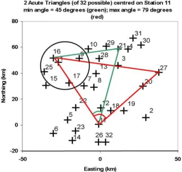
Fig. 8. The locations of the rain gauge stations (with station 11 at the origin) in the Black Forest used in this study, indicated by crosses. The two triangles based on station 11 are those with ex-treme angles selected from the 32 including station 11; these are used in the entropy calculation for validation, discussed in Sect. 3.3. The circled region includes gauges 1, 9, 17, and 25, whose means appear in Fig. 9.
4 Application of the methods
4.1 Data analysis – derived statistics of the observations
The model described above was applied to the set of se-lected stations in Baden-W¨urtemberg in South-West Ger-many, whose locations are shown in Figs. 1 and 8. Mean pre-cipitation amounts are highly variable in this region. Table 1 shows the estimated January and July dry-day probabilities and the mean precipitation amounts on wet days.
Figure 9 shows the annual cycle of the average daily pre-cipitation by month for a few stations. Note the different an-nual cycles exhibited by the relatively close stations, which are strongly linked to altitude. Locations 1 and 25 with low elevations both on the west side of the Black forest have a similar cycle, with highest precipitation amounts occurring in early summer. Station 9 at a higher elevation located on the top of the mountains is wetter and has an annual maxi-mum in winter; station 17 at an intermediate altitude has a nearly uniform mean. These differences present a challenge for multisite precipitation modelling.
Marginal distributions and the copula parameters were estimated for each month separately. Parameters of the marginal distributions describing wet amounts were esti-mated using the maximum likelihood method.
Table 1.Selected rainfall stations; extremes in each column in bold.
January July Nr Location Elevation p0 Mean p0 Mean
(m) (mm) (mm)
1 Achern 138 0.41 3.7 0.55 6.7
2 Albstadt
Burgfelden 911 0.48 4.1 0.55 7.5 3 Altensteig Wart 594 0.43 4.6 0.53 5.3 4 Althengstett
Ottenbronn 530 0.47 3.8 0.55 5.4 5 Elzach
Oberprechtal 480 0.45 7.0 0.54 9.0 6 Gutach i,Br,
Bleibach 302 0.47 5.2 0.54 8.7 7 Freudenstadt
Kniebis 875 0.39 10.0 0.49 9.6 8 Freudenstadt
(WST) 797 0.36 8.7 0.50 7.7
9 Forbach
Herrenwies 750 0.45 10.4 0.52 10.4
10 Weisenbach 200 0.46 6.7 0.54 7.1 11 Eschbronn
Mariazell 716 0.53 4.9 0.58 6.3 12 Fluorn Winzeln 660 0.52 7.0 0.61 7.4 13 Freudenstadt
Igelsberg 757 0.37 7.0 0.51 7.0 14 Furtwangen 870 0.40 9.2 0.50 8.8 15 Offenburg 153 0.47 3.5 0.57 6.3 16 Rheinau
Memprechtshofen 131 0.49 3.8 0.59 6.5 17 Oppenau 315 0.42 7.3 0.52 8.3 18 Oberndorf/Neckar 516 0.46 5.3 0.53 5.9 19 Rosenfeld 640 0.45 3.8 0.54 5.8 20 Rottenburg,
Bad Niedernau 349 0.50 3.3 0.55 5.7 21 Oberreichenbach 639 0.44 5.1 0.53 5.9 22 Wolfach 265 0.46 6.7 0.54 8.4 23 Triberg Nussbach 720 0.44 7.3 0.52 7.8 24 Triberg 683 0.43 9.3 0.49 8.8 25 Willst¨att
Legelshurst 140 0.54 3.5 0.62 6.8 26 Villingen
Schwenningen
(NST) 715 0.51 4.7 0.56 6.7
27 T¨ubingen
Bebenhausen 350 0.51 3.2 0.54 6.0 28 Enzkl¨osterle 600 0.43 7.8 0.52 7.4 29 Bad Wildbad
Sommerberg 740 0.41 7.2 0.50 7.0 30 Weil der Stadt 389 0.45 3.0 0.56 5.2
31 Tifenbronn 344 0.47 3.5 0.57 5.6 32 Villingen
Schwenningen 720 0.47 4.7 0.53 5.7
Fig. 9.Observed mean daily precipitation over the year for selected stations from the west of the cluster shown in Fig. 8; we note (by comparison with Fig. 1) that stations 1 and 25 lie in the low altitude area to the West, and that stations 9 and 17, although close, are sited at high and intermediate altitudes, clearly affecting the amount and patterns of rainfall.
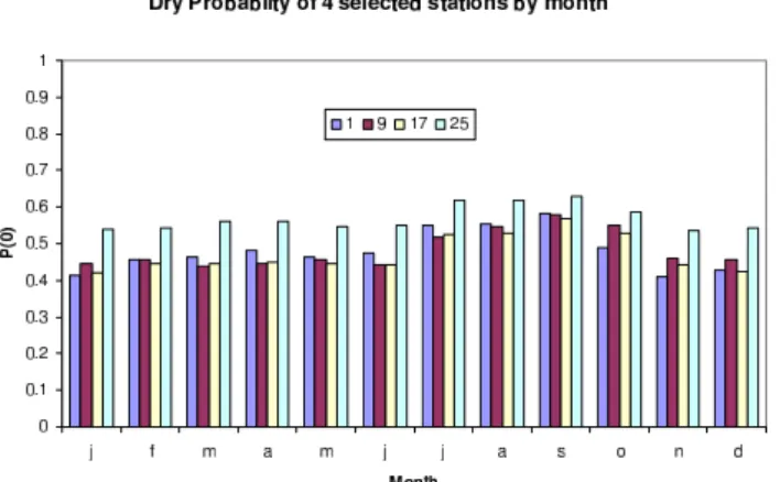
Fig. 10.The variation of the dry probabilities for 4 selected stations by month.
Fig. 11. The standard deviations of daily rainfall for selected sta-tions by month.
Fig. 12.Parameters of the copula transformation functiong.
Fig. 13. Serial correlations of the copula transformed y-variates determined from the data for stations 1 to 8.
The standard deviations of wet values of the same stations, shown in Fig. 11, vary in much the same way as the means shown in Fig. 9.
The spatial copula parameters (m,k, andα) are estimated for all gauges in the region each month using the multivariate copula; these appear in Fig. 12. This generalised treatment may need to be refined to allow the behaviour of individual gauges to be reflected in the model, but will add to com-plexity at this stage. Note the near constancy of the shift parameterm, with all months other than June and July hav-ing values of 1.91 and above. June and July experience more thunder-storms than the other months and havem=1.69 and 1.81, respectively. By contrast, the slopekof the right arm of the v-copula shown in Fig. 5, adjusts over the year to accom-modate the proportions of stratiform and convective rain, be-ing largest in the summer months.αneeds to be constrained and reaches its maximum of 3.5 over the first 6 months and December.
The serial correlations driving the y-variates of the hidden AR(1) multisite model are determined by maximum likeli-hood through the inverse of the V-copula transform. These temporal copulas are made to model the empirical temporal copulas like that shown in Fig. 7. The stations selected to display these hidden correlations appear in Fig. 13 and lie along the SW-NE diagonal in Figs. 1 and 8, except for sta-tions 1 and 2 which lie respectively in the extreme NW and SE. There is thus a good spread of behaviour as also indi-cated by the statistics in Table 1. Sites 7 and 8 are close to each other near the middle of Fig. 8 and show the highest (and most similar) correlations.
Spatial correlations of the copula-transformed y-variates seem to depend on distance, as well as altitude. We com-pute the monthly spatial cross-correlations of the Gaussian y-variates between sites 1–8 against site 30, as shown in Fig. 14, where the sites (1–8) have been ordered by their dis-tance from site 30 (the furthest NE site of the set of 32) which ranges from 10 to 97 km. We note that there is not much de-pendence of this statistic on annual variability; it varies more between sites.
The values in Fig. 14, which range from 0.76 to 0.98, are considerably higher than the correlations for the rain amounts obtained by the Srikanthan-Pegram (henceforth “covariance”) model, which range from 0.40 to 0.89 over the same set of station inter-associations exhibited in the figure. The (hidden) normal correlations for the occur-rences (wet/dry) process in the covariance model are much closer to those of the corresponding stations for the copula-based model, ranging from 0.80 to 0.96. These sets of val-ues are not strictly comparable because, in this paper we are using the multinormal correlations of variables reverse-transformed through the copula relationship, however, they are interesting.
It is not strictly fair to compare these with the intersite cor-relations of the hidden covariance model of Srikanthan and Pegram (2009). However, we will use that model in
eval-uating the efficacy of the entropy congregation criterion in the next subsection, so it worth outlining its philosophy here. The relevant passage from the abstract of that paper describes the model as a
multisite two-part daily model nested in multisite monthly, then annual models. A multivariate set of fourth order Markov chains is used to model the daily occurrence of rainfall; the daily spatial correlation in the occurrence process is handled by using suitably correlated uniformly distributed variates via a Normal Scores Transform (NST) ob-tained from a set of matched multinormal pseudo-random variates, ... a hidden covariance model. A spatially correlated two parameter gamma distri-bution is used to obtain the rainfall depths; these values are also correlated via a specially matched hidden multinormal process.
Figure 15 shows the scatterplots of the observed and sim-ulated interstation correlations and rank correlations of the rainfall amounts for winter. As one can see, the simulated correlations are slightly lower than the observed ones. In contrast, in the rank correlations there is no systematic dif-ference between the simulated and the observed series. The reason for this is that the copula approach is based on the rank correlations fitted in the transformed domain.
5 Results: comparison of simulations with observations
20 replicates of the historical series (effectively 860 years) were generated and certain statistics of interest were deter-mined from these and compared to the corresponding statis-tics of the historical series.
5.1 Calculation of distributional statistics
The performance of the model is demonstrated using differ-ent uni- and multi-variate statistics. Figure 16 shows the (smoothed) annual cycles of the averages of the historical and 20 simulated mean daily precipitation sequences, for a pair of selected stations (8 and 30), where it is seen that the values are satisfactorily recaptured, thus verifying this aspect of the model behaviour.
Fig. 15. Cross-correlations (circles) and rank cross correlations (crosses) for the observed and simulated precipitation series.
Fig. 16. Comparison of the averages of 20 simulated and the ob-served mean daily precipitation over the year for stations 8 and 30 – the average of the simulations is smoother, as expected.
The comparisons of observed and simulated conditional and unconditional cumulative distribution functions appear-ing in Figs. 17 and 18 show that the copula-based procedure captures the joint modelling of wet/dry and amounts pro-cesses well. Figure 19 displays the frequency of the numbers of gauges that are wet on any given day during winter; the results for summer are equally good. Again, because we are more concerned about heavier than lighter rainfall, the com-putations are performed by conditioning the observations on the higher 10 mm threshold. This will mean that there are likely to be more zero counts than if the threshold is set at the observation precision of 0.1 mm.
Fig. 17. Observed and (average of 20) simulated cumulative dis-tributions of daily precipitation for station 7 in winter (December– February). The upper solid lines are the unconditional cdfs. The dashed lines show the conditional distributions where the daily pre-cipitation at station 8 is not less than 5 mm. Black lines are the observed and the red lines are the simulated distribution functions using the V-copula. Note that in the upper line (unconditional cdf), theP[0] value of 0.39 for January given in Table 1 is closely cap-tured by the simulated series, obscured slightly by the step at the axis.
Fig. 19. Distribution of the number of 32 stations exceeding the threshold of 10 mm on a winter day:P[all stations<10 mm]=0.55.
Table 2.Joint triple probabilities of observations at stations 11, 16, and 21 being below (1) and above (2) quantile 0.90.
Stations
11 16 21 p(i,j,k) 1 1 1 0.8258 1 1 2 0.0239 1 2 1 0.0333 1 2 2 0.0170 2 1 1 0.0300 2 1 2 0.0203 2 2 1 0.0110 2 2 2 0.0387
5.2 Validation using entropy of triples
The calculation of the entropyH, as described in Sect. 3.4, for a given set of data is demonstrated in this section and then applied to the data-sets.
Recall that H = −P
{p(i,j,k).ln[p(i,j,k)]} summed over alli,j,k=1,2 for a given triple.
The red triangle in Fig. 8 has vertices at the points (11, 16, and 21) and over the record, the observed probabilities of the triple being jointly below or above the 0.90 quantile, (indicated by 1 or 2) in various combinations, are given in Table 2.
The probabilities are obtained by counting the number of occurrences of the three gauges’ quantiles being jointly above or below 0.9 on all days for the record of 42 years in the eight patterns.
Fig. 20. Isometric view of the 3-D probability space of the three stations (11, 16, and 21) being wet or dry, with the hidden all-dry probability indicated as 0.826.
The diagram in Fig. 20 indicates the arrangement, with the value of the hidden (all dry) probabilityp(1,1,1)=0.826 as indicated. If the gauged data were independent, p(2,2,2) would equal 0.13=0.001 instead of the observed 0.039. The observed relative value is a multiple of 39 greater than the independent one, indicating strong dependence between the high quantiles.
The entropy for the above triple is 0.790, less than the figure of 0.975 which would be calculated in the indepen-dent case for a quantile threshold of 0.90; this comparison indicates greater association between the data than indepen-dence. In contrast, the entropy of the completely dependent case would be 0.325, indicating maximum association be-tween the data.
Fig. 21. Entropies of Data and two models, the Copula model and the Covariance model, under the assumption thatP (0)=0.5, for the purpose of comparing models’ ability to model the wet/dry process. The entropy value for complete interdependence is 0.693 whenh=A=0.
Turning to the data in isolation from the simulations, Fig. 22 presents the entropy behaviour over the same network at three thresholds: dry/wet assumed to have quantiles of 0.5; 0.90 (repeated from Fig. 21) and 0.975. The entropy lower bounds are 0.693; 0.325; 0.117 for values of marginal quan-tiles 0.5; 0.9; 0.975, respectively. The fitted trend lines are guides, not suggesting structure, however the convergence of the (h, H) plots towards the corresponding dependence limits is more convincingly demonstrated by using lnA in place ofA1/2. The nearly equidistant behaviour of the en-tropy plots of the data in log-space suggest some underlying useful structure which we have yet to explore.
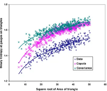
Finally, in Fig. 23, we present a comparison between the entropy behaviour of the three sets: (i) the data, (ii) the copula model simulations and (iii) the covariance model simulations for the 90% threshold. The Area of the red triangle in Fig. 8 joining points (11, 16, and 21) is 1411 km2. In Fig. 23 the corresponding point (h,H )= √
Area,entropy=(37.56,0.790)appears as a red dot. It is clear that the copula model is closer to the data across the range ofhthan the covariance model, but is still not close enough for a complete match, indicating that the congregat-ing behaviour of the copula simulations is an improvement over the covariance ones, but still needs attention. In partic-ular, this interdependence would be modelled by a high di-mensional copula. However, the discrimination between the sequences offered by the entropy measure is encouragingly sharp.
Fig. 22.Entropies of the observed Data at three quantile thresholds: 0.50, 0.90 and 0.975, and suggested convergence to the correspond-ing limits of complete interdependence.
Fig. 23.Entropies of the data and the Copula model and Covariance models, plotted as (h,H). All appear to converge to the value 0.325 of perfect dependence, indicated by the red line lower bound, when
h=A=0. The red dot is (h,H)=(37.56, 0.790) calculated at the start of this section, corresponding to the red triangle in Fig. 8.
The method indicates that the copula model is superior in this respect to the covariance model to which it was com-pared, but not yet good enough to suggest that it fully cap-tures the spatial structure of rainfall recorded in networks of gauges. To achieve this will require the application of a truly multi-dimensional copula, not one predicated on a combina-tion of bivariate relacombina-tionships.
6 Conclusions
The paper set out to establish the nature of the interdepen-dence between rainfall sequences in an inhomogeneous re-gion, to determine an appropriate model. It was found that the classical Normal Scores Transform is not rich enough to capture the range of correlations being strong at high rain-fall values and weak at low rainrain-fall amounts. Multinormal variables defined by their correlation structure were nonlin-early transformed, from which set the copulas were derived. The parameters of the transforms and the hidden correlations were obtained by using numerical optimisation to obtain the maximum likelihood. The resulting parameters were used with success in modelling both the rainfall amounts and the occurrences simultaneously.
A novel technique using entropy for determining the de-gree of congregation of wet gauges was devised which shows that the copula-based model is an improvement over the tra-ditional multisite covariance models, but that it still needs improvement to match the data. Other statistics used for vali-dation, such as cumulative distribution functions conditioned on neighbouring sites experiencing rainfall above a relatively wet threshold of 10 mm, show that these distributions are well mimicked by the copula-based multisite rainfall model.
Acknowledgements. Research leading to this paper was supported by the joint DFG-NRF program, project number Ba-1150/13-1.
Edited by: E. Todini
References
Akaike, H.: A new look at the statistical model identification, IEEE T. Automat. Contr., 19(6), 716–723, 1974.
Apipattanavis, S., Podest´a, G., Rajagopalan, B., and Katz, R. W.: A semiparametric multivariate and multisite weather generator, Water Resour. Res., 43, W11401, doi:10.1029/2006WR005714, 2007.
B´ardossy, A.: Copula-based geostatistical models for ground-water quality parameters, Water Resour. Res., 42, W11416, doi:10.1029/2005WR004754, 2006.
B´ardossy, A. and Li, J.: Geostatistical interpolation using copulas, Water Resour. Res., 44, W07412, doi:10.1029/2007WR006115, 2008.
Fang, H.-B., Fang, K.-T., and Kotz, S.: The meta-elliptical distribu-tion with given marginals, J. Multivariate Anal., 82, 1–16, 2002. Herr, D. and Krzysztofowicz, R.: Generic probability distribution of rainfall in space: The bivariate model, J. Hydrol., 306, 237–264, 2005.
Joe, H.: Multivariate models and dependence concepts, Chapman Hall, Boca Raton, 1997.
Linhart, H. and Zucchini, W.: Model Selection, Wiley, New York, 1986.
Matalas, N.: Mathematical assessment of synthetic hydrology, Wa-ter Resour. Res., 3(4), 937–945, 1967.
Mehrotra, R. and Sharma, A.: Preserving low-frequency variability in generated daily rainfall sequences, J. Hydrol., 345, 102–120, 2007.
Mehrotra, R., Srikanthan, R., and Sharma, A.: A comparison of three stochastic multi-site precipitation occurrence generators, J. Hydrol., 331, 280–292, 2006.
Nelsen, R.: An introduction to copulas, Springer Verlag, New York, 1999.
Pegram, G. and James, W.: A Multivariate Multi-lag Autoregres-sive Model for the Generation of Operational Hydrology, Water Resour. Res., 8, 1074–1076, 1972.
Press, W., Teukolsky, S., Vetterling, W., and Flannery, B.: Numer-ical recipes in Fortran, Cambridge University Press, Cambridge, England, 1992.
Salvadori, G., Michele, C. D., Kottegoda, N., and Rosso, R.: Ex-tremes in nature. An approach using copulas, Springer, New York, 2007.
Serinaldi, F.: Copula-based mixed models for bivariate rainfall data: an empirical study in regression perspective, Stoch. Env. Res. Risk. A., 23, 677-693, 2009.
Serinaldi, F.: Multisite generalisation of a daily stochastic precipi-tation generation model, Stoch. Env. Res. Risk A., 22, 671–688, 2008.
Sklar, A.: Fonctions de r´epartition `a N dimensions et leurs marges, Publ. Inst. Stat. Paris, 8, 229–131, 1959.
Srikanthan, R.: Stochastic Generation of Daily Rainfall Data at a Number of Sites, CRC for Catchment Hydrology, Technical Re-port 05/7, 7, 66, Monash University, 2005.
Srikanthan, R. and McMahon, T. A.: Stochastic generation of an-nual, monthly and daily climate data: A review, Hydrol. Earth Syst. Sci., 5, 653–670, 2001,
http://www.hydrol-earth-syst-sci.net/5/653/2001/.
Srikanthan, R. and Pegram, G.: A Nested Multisite Daily Rain-fall Stochastic Generation Model, J. Hydrol., 371(1–4), 142–153, 2009.
Thomas, H. and Fiering, M.: Mathematical synthesis of streamflow sequences for the analysis of river basins by simulation, Design of Water Resources Systems, Harvard University Press, Cam-bridge, MA, USA, Chapter 12, 1962.


![Fig. 19. Distribution of the number of 32 stations exceeding the threshold of 10 mm on a winter day: P [ all stations < 10 mm]=0.55.](https://thumb-eu.123doks.com/thumbv2/123dok_br/18157257.328336/14.892.470.801.93.376/fig-distribution-number-stations-exceeding-threshold-winter-stations.webp)