Firing and training costs and labour market segmentation

(1)

Universidade Nova de Lisboa

Thesis, presented as part of the requirements for the Degree of Doctor of Philosophy in Economics

Firing and training costs and labour market

segmentation

Sara Raquel Coelho Serra

Student Number 573

A Thesis carried out on the Ph.D. Program in Economics, under the supervision of Prof. Francesco Franco

(2)

(3)

Abstract of the thesis

This dissertation consists of three essays on the labour market impact of firing and training costs. The modelling framework resorts to the search and matching literature. The first chapter introduces firing costs, both linear and non-linear, in a new Keynesian model, analysing business cycle effects for different wage rigidity degrees. The second chapter adds training costs to firing costs in a model of a segmented labour market, accessing the interaction between these two features and the skill composition of the labour force. Finally, the third chapter analyses empirically some of the issues raised in the second chapter.

(4)

(5)

List of Tables

1.1 Model Calibration . . . 30

1.2 U.S. Business Cycle Data - Sources and Descriptive Statistics . . . 78

1.3 Business cycle properties of US economy and model economy: linear fir-ing costs . . . 79

1.4 Business cycle properties of US economy and model economy: asymmet-rical firing costs . . . 80

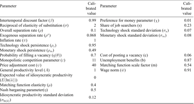
2.1 Calibrated Parameters . . . 119

3.1 Composition of employment by contract type . . . 213

3.2 Employer characteristics by contract type . . . 214

3.3 Transitions from temporary jobs . . . 215

3.4 IMD- Labour regulations indicator. . . 215

3.5 Descriptive statistics - Overall Sample . . . 216

(10)

3.8 Transitions - Results without unobserved heterogeneity. . . 219

3.9 Transitions - Results with unobserved heterogeneity . . . 220

3.10 Transitions to an open-ended contract with the same employer- Results with un-observed heterogeneity, by country group . . . 221

3.11 Transitions to an open-ended contract with a new employer - Results with unob-served heterogeneity, by country group . . . 222

3.12 Transitions to joblessness - Results with unobserved heterogeneity, by country group . . . 223

3.13 Transitions between temporary jobs - Results with unobserved heterogeneity . . 224

(11)

List of Figures

1.1 Timing of events in the labour market . . . 14

1.2 Steady-State Comparison . . . 33

1.3 Impulse response functions to a 1% technology shock and different degrees of wage rigidity and firing costs . . . 64

1.4 Impulse response functions to a 1% monetary shock and different degrees of wage rigidity and firing costs . . . 68

1.5 Impulse response functions to a 1 standard deviation productivity shock with asymmetrical firing costs . . . 72

1.6 Impulse response functions to a 1 standard deviation monetary shock with asym-metrical firing costs . . . 75

2.1 Labour market flows . . . 103

2.2 Steady-State response to a permanent productivity shock in open-ended contracts . . . 152

(12)

employment . . . 153

2.5 Transitional dynamics - overall productivity shock . . . 153

2.6 Steady-State response to a permanent training cost shock . . . 154

2.7 Transitional dynamics - Training cost shock . . . 154

2.8 Steady-State response to a shock in the initial level of skill . . . 155

2.9 Transitional dynamics - Initial skill level shock . . . 155

2.10 Steady-State response to a permanent shock on firing costs of open-ended contracts . . . 156

2.11 Transitional dynamics - permanent contracts’ firing costs shock . . . 156

2.12 Steady-State response to a permanent shock on firing costs of temporary contracts . . . 157

2.13 Transitional dynamics - temporary contracts’ firing costs shock . . . 158

2.14 Steady-State response to a permanent shock in both types of firing costs . 158 2.15 Transitional dynamics - shock on firing costs of both types of contracts . . 159

2.16 Tradeoff between training costs and length of a temporary contract forφ= 1159 2.17 Tradeoff between training costs and firing costs in permanent contracts forφ= 1 . . . 160

(13)

Acknowledgments

First of all, I would like to express my gratitude to my advisor Prof. Francesco Franco for his guidance and insight over the development of this project, where he has provided me the freedom to pursue my research interests while upholding high standards about the quality of the output. I also would like to thank Prof. Pedro Portugal for helpful suggestions and fruitful discussions, particularly regarding the third chapter of this thesis.

To all the participants in the Informal Research Workshop and PhD research group at Nova School of Business and Economics, who have provided valuable input throughout my work, I would also like to express my appreciation. I also benefited from the comments and suggestions of the participants of the 2014 QED conference and of seminars at Banco de Portugal.

Thanks also to my colleagues at the PhD programme, especially Ana Gouveia, Ana Rita Mateus, Daniel Carvalho and Luciana Barbosa, whose team work and support helped me reach this point of this journey.

(14)

My deep gratitude to family and friends for their endless patience and support through-out this long journey.

Lastly, but foremost, to Fernando Dordio, for everything.

Sara Serra

(15)

Introduction

The three essays that compose this dissertation focus on the interaction between the labour market and institutions, namely employment protection legislation (EPL) in the form of firing costs, and human capital issues, also conditioned by training costs. This analysis is pursued through a modelling framework that is largely based on the new Keynesian and search and matching literature. Two of the essays address directly the context of seg-mented labour markets which is a reality in several European countries. The first chapter analyses the business cycle impacts of introducing linear and non-linear firing costs in a new Keynesian model with different degrees of wage rigidity. The second chapter is based on a model of a segmented labour market in which both firing and training costs are present. The interaction between these two features and the skill composition of the labour force is analysed in this chapter. Finally, the third chapter analyses empirically some of the issues raised in the second chapter, namely the impact of employment protection and human resources policies on the type of contractual relationships prevailing in the labour market.

(16)

this analysis by adding firing costs to this setup, in isolation and in interaction with wage rigidity. In a first approach, firing costs are considered to be linear, as commonly assumed in the literature. However, this assumption does not take into account that increasing separations may have intangible costs, like loss of job-specific human capital, which do not translate into symmetrical benefits when separations are reduced. It can also be viewed partially as a proxy for labour market regulation in a segmented labour market, where for a small number of dismissals only workers with fixed-term contracts with low firing costs are affected, while for high separation rates employees with open-ended contracts are also impacted. This chapter proposes an asymmetrical firing cost function as a reduced form to address this problem, and evaluates the impact of its implementation in the model and its business cycle properties. This setup allows for an improvement of the business features of the model when compared to the baseline similar to the one obtained with linear firing costs, but the response of output to monetary policy shocks is now asymmetrical and more muted in the case of a contractionary shock.

(17)

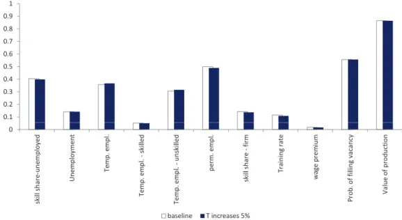
impor-tant aspect to bear in mind, and so far relatively neglected in the literature. Although the consequences for economic growth are not addressed in the work, the analysis offers some insight on this issue. Results emphasize the analysis of the impact of recent and possible future reforms in European labour markets, showing that a policy along the lines of the single contract can have benefits in terms of increased employment and higher average skill level in the economy.

The third chapter tries to assess empirically one of the main assumptions of the second chapter, namely the nexus between training and transitions from fixed-term to open-ended contracts or to joblessness in Europe and how it is affected by employment protection leg-islation. In the analysis, intra and inter-firm transitions between temporary and permanent contracts are distinguished, a feature not explored in the literature. Results signal the pos-itive impact of training and of the flexibility of labour regulations on transitions from tem-porary to permanent contracts, particularly in segmented labour markets. A strong feature of the results is that workers with a sequence of temporary jobs have a lower probability of making a transition both to permanent employment and to unemployment, suggesting the persistence of this form of contract in the careers of some workers.

(18)

(19)

Chapter 1 Firing costs and real wage rigidity in a

New Keynesian model

Abstract

Although the introduction of the search and matching framework in New Keynesian mod-els has been successful, some caveats remain. Namely, these modmod-els fail to replicate some labour market stylized facts, as the negative correlation between vacancies and unemploy-ment, the so called Beveridge curve. This paper introduces in such a setup the impact of employment protection legislation, namely firing costs, along the lines of Krause and Lu-bik (2007). The impact on business cycle dynamics of this relevant factor for European labour markets, as well as the interaction of this feature with real wage rigidity, is analysed in this paper. As an original contribution to the literature, the impact of non-linear firing costs is also object of analysis. Conclusions suggest that the introduction of firing costs in the model improves some business cycle features of models in this framework, although it maintains limitations in other aspects, like the estimated correlation between job flows.

JEL Classification: E24, E32, J64.

(20)

1.1 Introduction

Real Business Cycle and later New Keynesian models have become the reference eco-nomic models as regards business cycle analysis. However, in their initial versions, these models presented some limitations as to replicate business cycle facts. Given the impor-tance of the labour market for welfare and policy definition, a serious shortcoming of these models was the absence of unemployment in equilibrium, as the labour market was usu-ally modeled as frictionless. In an attempt to circumvent this limitation, more recently a labour market framework characterized by search and matching frictions (Mortensen and Pissarides (1994)) has been integrated in New Keynesian models (Trigari (2006), Blan-chard and Galí (2010) and Christoffel et al. (2009) among others). The generalization of this approach to labour market modelling reflects some interesting features, like the presence of rational expectations, optimizing agents and a focus on flows into and out of unemployment. Although the matching function, that describes the process through which workers and firms meet in the labour market, lacks microeconomic foundations, the simplicity of its functional form and the fact that it is validated by the data (Petrongolo and Pissarides (2001)) also contributed to the popularity of this approach. Although the search and matching framework has helped to improve the business cycle properties of New Keynesian models, some empirical regularities are not yet replicated by the model, namely the volatility of vacancies, the negative correlation between this variable and un-employment (usually designated as the “Beveridge curve”) and between job creation and job destruction rates.1 _{In addition, Christoffel et al. (2009) analyze the several variants of}

New Keynesian models with a search and matching framework available in the literature (right-to-manage, on-the-job search, endogenous destruction, etc.) and conclude that in general these models provide a response of inflation to monetary shocks that is much more volatile than in the data. They conclude that the model that most successfully addresses this problem combines right-to-manage bargaining with nominal wage stickiness. Other 1_{See Yashiv (2007) and Hornstein, Krusell and Violante (2005) for a survey of the search and matching}

(21)

works have tried to solve the empirical problems of the search and matching framework, in particular the muted response of unemployment and vacancies to productivity shocks, by adding wage rigidity, as in Hall (2005). However, Hornstein et al. (2005) argue that this approach also originates some results at odds with empirical evidence. Moreover, Krause and Lubik (2007) claim that although full wage rigidity allows a New Keynesian model with search and matching frictions to generate a Beveridge curve, other issues remain, namely as regards inflation persistence.

(22)

rele-vant (see Garibaldi and Violante (2005) for a computation of these costs for the case of the Italian economy), Emerson (1988) reports that for every country surveyed the redundancy payments related to dismissal were considered to be less important than the length of no-tice periods and the difficulty of legal procedures. Normally in the context of search and matching models only the costs that do not constitute a severance payment are considered, given that the effect of the transfer from firms from to workers could be in theory contrac-tually annulled in an environment of rational, risk-neutral agents (see Lazear (1990) for an illustration). This is also the approach followed in the current work.

Some papers have combined to some extent the strands of the literature related to firing costs and some form of wage rigidity: Garibaldi and Violante (2005) prove that the above mentioned neutral effect of a severance payment does not hold under wage rigidity. Cahuc and Zylberberg (1999) conclude that the same is true when the hypothesis that wage rene-gotiations take place every period is dropped and Cassorla (2010) analyzes the interaction of firing costs and minimum wages.

In the above mentioned approaches to firing costs, these are considered to be linear, resulting in a cost of increasing separations which is identical to the savings for the firm by reducing them. However, increasing separations may carry effects other than the monetary ones, as loss of human capital (see Ljungqvist and Sargent (2005) for an application of the search and matching framework with loss of worker skills upon layoff) or loss of worker morale (Bewley (1995)). Several microeconomic studies have found evidence of asymmetry in costs of labour adjustment, despite measurement issues that hinder this analysis, because many of these costs are “internal”, given that they are translated into changes in production but not directly measurable (see Hamermesh and Pfann (1996) for a survey of the literature).2

As a proxy for these effects, we implement an asymmetrical firing cost function,

ac-2_{These results are not however directly transposable to the current framework given that labour}

(23)

cording to which increases in the separation rate amount to higher costs than the benefits induced by a reduction. Moreover, the costs are higher the larger the size of the increase in the separation rate, such that abrupt variations are more penalized than gradual ones, i.e, the cost function is convex. This approach is an application to firing costs of the work by Kim and Ruge-Murcia (2009) and Fahr and Smets (2010) regarding downward wage rigidity.

The current paper follows closely Krause and Lubik (2007) and to a smaller extent Walsh (2003) and den Haan, Ramey, and Watson (2000), adding to the setup of these models linear firing costs, along the lines of Zanetti (2011) or Thomas and Zanetti (2009). The current work differs from these references by analyzing the effects of productivity and monetary shocks not only with firing costs and wage rigidity considered separately, but also the interaction between these two features. In addition, the impact of introducing asymmetrical firing costs in the model is also analysed.

We conclude that firing costs, both in their linear and non-linear form, help to improve some of the results of a New Keynesian model augmented with search and market fric-tions, namely by replicating the negative correlation between unemployment and vacan-cies present in the data while requiring a less strict assumption than the full wage rigidity hypothesis in Krause and Lubik (2007). However, they do not contribute to replicate other features of the data, namely the persistent response of inflation to monetary shocks. The model that presents the best overall performance as concerns business cycle proper-ties combines firing costs and wage rigidity, suggesting that further research is needed on interaction between labour market institutions.

(24)

1.2 Model

1.2.1 Model with Linear Firing Costs

The baseline model largely follows Krause and Lubik (2007), whose results are taken to be a starting point of the analysis. Some details of the model, namely the law of motion for employment and the timing of events in the labour market, follow den Haan et al. (2000).

Households

There is continuum of households in the unit interval. Each household is composed of em-ployed and unemem-ployed agents and maximizes its expected lifetime utility at timet, given by the functionUt, which depends on real consumption (c) and the real stock of money

(_M

P

)

. For this optimization problem the only relevant constraint is the aggregate resource level of the household, an assumption that allows us to abstract from distributional issues among employed and unemployed agents.3 _{The labour supply is fixed at one (therefore}

labour force equals population). Therefore, given that there are(e)employed workers, the remaining(1-e)agents are unemployed. The fact that the labour force is standardized to unity allows probabilities associated to labour market events and the corresponding labour flows to be identical in this model.

Therefore, the problem faced by the representative household is the following:

max {

ct,Mt_Pt,Bt_Pt

}∞

t=1 ¯

Ut=E0 ∞

∑

t=0 βt

[

c1t−σ−1

1−σ +χln Mt

Pt

]

(1.1)

3_{Alternatively, the consumer problem for employed and unemployed agents could have been modelled}

(25)

subject to the folllowing budget constraint (expressed in real terms, where high case letters denote nominal variables, while low case letters denote real variables):

ct+

Mt

Pt

+Bt

Pt

≤wtet+

Mt−1 Pt

+it−1 Bt−1

Pt

+b(1−et) +

P roft

Pt

+ Tt

Pt (1.2)

where β is the intertemporal discount factor of the household, which is assumed to be

constant, andM andB are nominal money holdings and bonds, respectively. Note that

given that the economy is closed, in equilibrium the supply of bonds will equal demand

and bond holdings will be zero on average. Bonds yield a gross interest rateiper period

and w and b represent the wage rate and unemployment benefits of the employed and

unemployed members of the household, respectively.Pstands for the average price level,

Prof are the profits of the firms accruing to the household andT are transfers from the

state.

The Lagrangian for the consumer problem is given by:

L₍_c_t_{, m}_t_{, b}_t_{, λ}_t_{) = ¯}_U_t₊

E₀

∞ ∑

t=0

βtλt

[

wtet+mt−1

Pt−1

Pt

+it−1bt−1

Pt−1

Pt

+b(1−et) +P roft+Tt−ct−mt−bt

]

givenb−1= ¯b, m−1= ¯m

(26)

The first order conditions to this problem are:

∂L

∂ct

= 0⇔c−_tσ =λt (1.4)

whereλtis the shadow value of an additional unit of income to the the household, thus implying

that in equilibrium it equals the marginal utility of consumption.

∂L

∂mt

= 0⇔χ 1

mt

+βEt

[

λt+1

Pt Pt+1

]

−λt= 0 (1.5)

This condition implies that the marginal utility of holding money equals the utility cost of

de-laying consumption one more period.

∂L

∂bt

= 0⇔βEt

[

λt+1it Pt Pt+1

]

−λt= 0 (1.6)

The first order condition regarding bonds implies that at the margin the consumer should be

indifferent between consuming an unit of income today or investing it in bonds that yield a gross

interesti.

Finally, the remaining first order conditions are given by:

∂L

∂λt

λt= 0;

∂L

∂λt

(27)

And the transversality conditions are given by:

lim

j→∞β

j_E

t[λt+jbt+j] = 0; lim

j→∞β

j_E

t[λt+jmt+j] = 0 (1.8)

Replacing (1.4) on (1.6) we obtain the definition of the nominal interest rate:

βEt

[

c−_t₊₁σit Pt Pt+1

]

=c−_tσ ⇔it=Et

([

ct+1

ct

]σ Pt+1

Pt

1

β

)

=Et

([

ct+1

ct

]σ πt+11

β

)

(1.9)

whereπt= _ptpt−1 defines the inflation rate.

Replacing (1.4) on (1.5) we obtain the equation for the demand for money, which depends on

transaction and speculative motives:

mt=χ

it

it−1

cσ_t (1.10)

The supply of real money balances is given by:

mt=mgtmt−1 (1.11)

where:

ln(mgt) =ρmln(mgt−1) +εmt (1.12)

(28)

Given equations (1.10) and (1.11), the equilibrium condition in the money market can be written

as:

it it−1

=mgt

it−1

it−1−1

(

ct ct−1

)−σ

1

πt

(1.13)

which implies that the change in the nominal interest rate is a function of money growth, past

interest rates, consumption growth and inflation.

Final Goods Firms

The household buys a final composite good that is the result of the assembly of a continuum of

intermediate goods. We depart from Krause and Lubik (2007) in assuming that the assembly of

these intermediate goods is carried out not by the household but by a final goods firm behaving

competitively. This distinction, which is mostly formal, allows a clearer separation between the

production and expenditure approaches to GDP calculation. The final goods firm bundles the

intermediate goods according to the following rule:

Yt=

(∫ 1

0

y ε−1

ε

it di

) ε

ε−1

(1.14)

whereyi represents the amount of goods of typei, i.e., produced by firmi, andYt is the final

consumption good. In equilibrium, the demand by the final goods firm of each of the intermediate

goods is given by (see the Appendix for a derivation):

yit =

(

Pt Pit

)ε

(29)

Replacing equation (1.15) in (1.14) the following expression for the general price levelP is

obtained:

Pt=

[∫ 1

0

P_it1−εdi

]₁−1ε

(1.16)

Intermediate Goods Firms

The intermediate goods firms are responsible both for the pricing and labour demand decisions in

the economy.

As regards the characterization of the production and labour market frameworks, the variable

ncorresponds to the beginning of period number of employment relationships or jobs. These

in-clude both previously employed workers and new matches that were formed in end of the previous

period. Each period wages are (re)negotiated. Each agentjwithin an employment relationship

in firmiis associated to a general productivity levelA, and to a specific productivity level aij,

which is an independent and identically distributed (both across time and across agents) stochastic

variable with cumulative distribution functionF(aij)and positive support. The production

func-tion depends linearly on labour, and therefore in periodteach agent involved in an employment

relationship potentially producesyijt=Ataijt.

The law of motion ofAtis given by:

ln(At) =ρzln(At−1) +εzt (1.17)

(30)

The decision of a firm to employ a given agent in periodtcan be summarized by the following

Bellman equation:

V_ijtJ =max{−δ, Ataijt−wijt+βEtVijtJ+1} (1.18)

whereδis the firing cost per separation.

By the envelope condition,

∂VijtJ

∂aijt

=At>0

The value function is increasing in the job-specific productivity level, and consequently the

relevant decision for the firm will be a threshold level˜aitsuch that above that level employment

relationships will be maintained and below will be severed. Therefore, the probability of an

em-ployment relationship being endogenously severed is given byρn

it = P r[ait < a˜it] = F(˜ait).

Additionally, there is a probability of exogenous separation given byρx. Assuming that

exoge-nous separations happen before the endogeexoge-nous, the overall probability of separation is given by:

ρit=

ρxnit−1+ρitn(1−ρx)nit−1 nit−1

=ρx+ (1−ρx)F(˜ait) (1.19)

wherentis the number of jobs (employment relationships existent prior to production).

Given this, actual employment (resources used in production) is defined as:

(31)

And the aggregate production of firmiis given by:

Yit=At(1−ρit)nit−1E[ait|ait>˜ait]⇔Yit=At(1−ρit)nit−1

∫ ∞

˜

ait

1−F(˜ait)

f(ait)dai≡

At(1−ρit)nit−1H(˜ait) =AtetH(˜ait)

(1.21)

After production has taken place in periodt, each firm adjusts (if deemed necessary) the number

of vacanciesvitit wishes to post in the labour market, and subsequently a number of new matches

is attributed to firmi, according to the following matching function:

m(st, vt) =msµtv

1−µ

t (1.22)

wherem is a scale parameter that denotes matching efficiency and st = 1 −(1−ρt)nt−1 is

the number of “searchers” in the labour market, i.e., agents looking for a match, which includes

both agents that were unemployed in the beginning of the period (ut = 1−nt−1) and agents

whose jobs was severed during periodt(a total ofρtnt−1 agents). Note that matching depends

on aggregate labour market variables(vt=

∫1

0 vitdi

)

, therefore giving rise to thick market and

congestion externalities. Given that the matching function has constant returns to scale, it can be

written as:

m(st, vt) vt

=m

(_s

t vt

,1 )

=q(θt) (1.23)

where labour market tightness is defined asθt = vt_st, the relative share of vacancies to searchers,

(32)

a job. Given this, the law of motion of jobs is given by:

nit = (1−ρit)nit−1+vitq(θt) (1.24)

or in terms of actual employment:

eit+1 = (1−ρit+1)[eit+vitq(θt)] (1.25)

The timing of events in the labour market is summarized in Figure 1.1 and follows den Haan

et al. (2000).4

Figure 1.1:Timing of events in the labour market

NtͲ1employment atisdrawn separations productiontakesplace newmatchesm(st,vt) Nt=(1Ͳʌt)NtͲ1+m(st,vt) at+1 separations productiontakesplace relationshipsexist takeplace with areformed employment isdrawn takeplace with

(1Ͳʌt)NtͲ1jobs relationshipsexist (1Ͳʌt+1)Ntjobs

(1Ͳʌt)NtͲ1jobs newvacanciesvt (1Ͳʌt+1)Ntjobs newvacanciesvt+1

remainavailable remainavailable areposted forproduction forproduction

PeriodT PeriodT+1

Considering that costs per separation are given byδ, total expected firing costs, considering

that all separations are affected, are given by:5

F Cit=ρitnit−1δ =

ρit

1−ρit

eitδ (1.26)

4_{This approach differs (although only formally) from the one of Krause and Lubik (2007) because}

in their model the variablen corresponds to actual employment (postseparation) while in this paper it corresponds to employment relationships (preseparation).

5_{Alternatively, the case where exogenous separations are not subject to firing costs could also be}

(33)

The problem of the firms is given by real profit maximization subject to (1.15), (1.21) and

(1.25):

max {ait,nit,vit,Pit,yit˜ }∞

0

E0

∞ ∑

t=0

βtλt λ0 [

Pit Pt

yit−wit(1−ρit)nit−1−vitc

−ψ 2

( _P

it Pit−1

−π

)2

Yt−ρitnit−1δ ]

(1.27)

subject to:

yit =

(_P

t Pit

)ε Yt

yit =At(1−ρit)nit−1H(˜ait) =AtetH(˜ait)

nit= (1−ρit)nit−1+vitq(θt) =eit+vitq(θt)

0≤nit≤1

wherewit=

∫∞

˜

aitw(ait) f(ait)

1−F(˜ait)daitis the average wage rate of firmi, given that a different wage will be paid to each employee as a function of his idiosyncratic productivity level. There is also

a quadratic adjustment cost term associated with price deviations from objective inflationπ, as in

Rotemberg (1982), that will lead to price rigidity in the model. Alternatively, price rigidity could

have been introduced through the Calvo (1983) price-setting mechanism. However, the Rotemberg

approach has the advantage of giving rise to a symmetric equilibrium, while the results do not differ

much from the Calvo setup given the appropriate calibration, as pointed out by Zanetti (2011).

(34)

of the constraints above and thatEt(βt+1) = Et(βλt+1/λt)is the intertemporal discount factor

betweentandt+1(which expresses profits in terms of the value to households, which own firms),

the first order conditions for this problem are (the problem is formalized in the Appendix):

∂L

∂nit

= 0⇔ξit=Et[βt+1(1−ρit+1) (ϕit+1At+1H(˜ait+1)−wit+1+ξit+1) +ρit+1βt+1(−δ)]

(1.28)

This intertemporal condition implies that the value of an employment relationship in period

t(ξit) should equal the expected discounted value of an employment relationship in periodt+1.

If the job is not severed in period t+1, which happens with probability (1 −ρit+1), the value

of an employment relationship in period t equals its continuation value, which consists of the

corresponding asset value, plus the flow of income it generates, (ϕit+1At+1H(˜ait+1)−wit+1).

With probability (ρit+1) the job is severed and the value of the employment relationship is negative

and amounts to the firing costδ.

∂L

∂vit

= 0⇔c=q(θt)ξit (1.29)

The first order condition for vacancies simply states that the cost of posting a vacancy equals the

corresponding expected benefit. This consists of the value of an employment relationship adjusted

by the probability that the vacancy is filled.

∂L

∂˜ait

= 0⇔

[

ϕitAtH(˜ait)−wit+ξit+δ

]

∂ρit

∂˜ait

= [

ϕitAt

∂H(˜ait) ∂˜ait

−∂w(H(˜ait))

∂˜ait

]

(35)

(1.30)

In equilibrium the net marginal cost of increasing˜aitequals the marginal benefit. The marginal

cost comprises the value of those employment relationships severed and the firing cost associated to

dismissal. The marginal benefit results from the increase in average productivity of the remaining

jobs net of the marginal change in the average wage.

∂L

∂Pit

= 0⇔ 1

Pt

yit−ψ

(

Pit Pit−1

−π

) 1

Pit−1

Yt−Et

[

ψβt+1

( −Pit+1

P_it2

)(

Pit+1

Pit

−π

)

Yt+1 ]

−εζit

(

Pt P_it2

)(

Pt Pit

)ε−1

Yt= 0

(1.31)

The optimality condition for the price level takes into account the additional income generated

by a marginal increase in prices when the current production level isyit, as well as the impact of

this increase on demand given the monopolistic competition setup and the price adjustment costs

in periodstandt+1.

∂L

∂yit

= 0⇔ζit=

Pit Pt

−ϕit (1.32)

Finally, the condition for the optimal production level simply implies that marginal revenueζit

(36)

Equations (1.28) and (1.29) give rise to the job creation condition:

c=q(θt)Et

[

βt+1(1−ρit+1) [

ϕit+1At+1H(˜ait+1)−wit+1+

c q(θt+1)

]

−βt+1ρit+1δ ]

(1.33)

This condition states that the cost of posting a vacancy equals the expected value of an

em-ployment relationship, which is created with probabilityq(θt). This employment relationship will

accrue income to the firm next period, when it is used for production. This consists of the value

of employment if the job is not severed (with probability(1−ρit+1)) and the cost δ otherwise

(with probabilityρit+1). The value of employment includesEt

(

c q(θt+1)

)

, which is the

continua-tion value of the job, i.e., the expected discounted stream of income that the job will generate in

the future if not severed.

This equation can be expressed as a function of the expected real marginal costEt(ϕit+1):

Et(ϕit+1) =Et

[(

c q(θt)

+βt+1ρit+1δ−

c q(θt+1)

βt+1(1−ρit+1)

)

1

At+1H(˜ait+1)

1

βt+1(1−ρit+1) ]

+Et

(

wit+1

At+1H(˜ait+1) )

(1.34)

The last term on the right hand side equals real unit labour costs. The first term in round

brackets, which is larger than unit in steady-state, translates the fact that the presence of search

and matching frictions leads to an increase in expected marginal costs, as a firm cannot ascertain

that a vacancy will be filled in the period it is posted given that this happens only with probability

q(θt). This implies that the average duration of an open vacancy is _q₍1_θt₎ and therefore the total

expected cost associated to a vacancy is c

(37)

making employment relationships costly even when they are not selected to production. This setup

reduces the value of an employment relationship when compared to a frictionless environment.

Equation (1.30) yields, after some algebra, the job destruction condition (see the Appendix for

details):

ϕitAt˜ait−w(˜ait) + c q(θt)

=−δ (1.35)

The termϕitcaptures the fact that an increase in output does not imply a one to one gain in revenue

due to the monopolistic competition setup. Condition (1.35) implies that the real profits generated

by the job with productivitya˜plus the continuation value of the job equals the firing cost. This

means that the firm is indifferent between employing or dismissing the worker with productivity

˜

a.

Replacing equation (1.32) in equation (1.31) and simplifying, we obtain the new Keynesian

Philips curve (see the Appendix for the complete derivation):

1−ψ

(

πit−π

)

πit+Et

[

ψβt+1

(

πit+1−π

)

πit+1

Yt+1

Yt

]

=ε(1−ϕit) (1.36)

Due to the symmetry of firms, all firm specific equilibrium conditions are also economy wide

conditions, and therefore the subscriptiis dropped henceforth.

Labour market

The labour market is characterized in this model by the equations describing the asset values for

(38)

having a filled or a vacant job. In addition, the bargaining process between workers and firms

determines wages. These conditions are composed of a flow of income resulting from being in a

given state at timetand the expected discounted asset value of that state in the following period.

The derivation of these laws of motion for the representative household and intermediate goods

firm problems can be found in the Appendix.

In the case of a worker employed at timet, the flow of income accruing to him is the wage

rate. In the following period, the worker will receive at least the value of his outside option,

corresponding to the state of unemployment. In addition, with probability(1−ρt+1), the match

will not be severed and the worker will also obtain the additional value of being employed int+1,

Wt+1, has in excess of the other possible state. Given that the match was not severed, this expected

value implicitly ranges over values of idiosyncratic productivity above˜at+1. Therefore, the value

of being employed can be expressed as:

Wt(at) =w(at) +Et[(βt+1(1−ρt+1)Wt+1+βt+1ρt+1Ut+1)|at+1>˜at+1]⇔

Wt(at) =w(at) +Et

[

βt+1(1−ρt+1)

∫ ∞

˜

at+1

( _W

t+1

1−F(˜at+1)

− Ut+1

1−F(˜at+1)

)

f(a)da+βt+1Ut+1 ]

(1.37)

where the last equality makes use of the fact thatUt+1does not depend on˜at+1.

The value function for an unemployed worker includes the unemployment benefit received at

timet. In the end of periodt, with probabilityθtq(θt), the agent is associated with a match, but this

is only converted into actual employment with probability(1−ρt+1), in which case he receives

(39)

the asset value in period t+1,Ut+1.

Ut=b+Et

[

βt+1θtq(θt)(1−ρt+1)

∫ ∞

˜

at+1

( _W

t+1

1−F(˜at+1)

− Ut+1

1−F(˜at+1)

)

f(a)da+βt+1Ut+1 ]

(1.38)

Regarding the value of a job for a firm (Jt), this has associated a stream of income at time

tcomposed of the real value generated by the job net of wage costs. The following period the

asset value of the job will correspond to the discounted value of the outside option, the value of

a vacancy. If the job is maintained (with probability(1−ρt+1)), the firm receives the additional

value it has vis-à-vis the outside option of a vacancy. In addition, the firm will pay a firing costδ

if the job is severed:

Jt(at) =ϕtAtat−w(at) +Et

[

βt+1(1−ρt+1)

(∫ ∞

˜

at+1

(

Jt+1

1−F(˜at+1)

− Vt+1

1−F(˜at+1)

)

f(a)da

)]

+Et(βt+1Vt+1)−Et(ρt+1βt+1δ)

(1.39)

Finally, posting a vacancy has a costcper period, and yields the net asset value of a job in the

following period,Jt+1−Vt+1, with probabilityq(θt)(1−ρt+1). In addition, the firm obtains its

outside option, the value of maintaining that vacancy open in the following period,Vt+1.

Vt=−c+q(θt)Et

[

βt+1(1−ρt+1)

(∫ ∞

˜

at+1

(

Jt+1

1−F(˜at+1)

− Vt+1

1−F(˜at+1)

)

f(a)da

)]

+Et(βt+1Vt+1)−Et[q(θt)ρt+1βt+1δ]

(40)

Given that separations affect all matches and not only employed workers, if a vacancy is filled,

but severed in the following period (before production takes place), the firm also has to pay firing

costs. The creation of a match implies in this framework a precommitment on both parties that

yields a compensation by the firm if it abandons the bargaining table. The assumption that only

wage renegotiations are affected by firing costs would require the need to consider the problem

of newly hired and continuing workers separately, as in Zanetti (2011). This would complicate

the analysis without significant changes to the overall economy results, given the likely reduced

relative share of new versus continuing workers. This assumption, however, affects wage

deter-mination, as described below.

Given that firms always enter the labour market by posting a vacancy, the assumption of free

entry in this market implies that in equilibriumVt(at) = 0 ⇒ Et[Vt+1(at+1)] = 0. Given this,

equation (1.40) becomes:

Et

[( _c

q(θt)

+(ρt+1βt+1δ)

)

1

βt+1(1−ρt+1) ]

=Et

[∫ ∞

˜

at+1

Jt+1f(a)

1−F(˜at+1)

da

]

(1.41)

This expression, along with equation (1.39), implies:

J(at) =ϕtAtat−w(at) + c q(θt)

(1.42)

Due to firing costs, if a match is not turned into a job or a job is not maintained, the firm will

incur in a loss ofδper separation. Given this, the firm will be willing to accept a wage that implies

a negative surplus from a job, as long as it is smaller than the corresponding firing costs to be paid.

(41)

levelatis therefore:

J(at)−Vt≥ −δ ⇔J(at)−Vt+δ≥0

This condition, evaluated at the threshold˜at, considering equation (1.42), yields exactly the job

destruction condition given by equation (1.35).

Wage determination is considered to be the result of a process of bargaining between the worker

and the firm in order to share the economic rents arising from their match. This is assumed to

be achieved through Nash Bargaining. The fact that the workers are aware of the structure of

the problem faced by firms leads firing costs to affect the relevant threat point of firms in the

Nash Bargaining problem.6 _{Therefore the relevant Nash Bargaining problem, with defines the}

equilibrium wage, is given by:

max

w(at)(Wt(at)−Ut)

η₍_J

t(at)−Vt+δ)(1−η) (1.43)

The first order condition of this problem implies the Nash Bargaining optimality condition (see

the Appendix for the derivation):

(1−η)[Wt(at)−Ut] =η(Jt(at)+δ) (1.44)

This condition is consistent with the assumption that firing costs apply to all bargaining

ne-gotiations, independently of whether the worker and the firm meet for the first time or simply

renegotiate wages. In fact, that Ljungqvist (2002) proves that assuming that firing costs affect

6_{See Cassorla (2010) and the references herein for a description of the application of Nash bargaining}

(42)

Nash bargaining when wages are renegotiated but not when the worker and firms first meet, as

in Garibaldi and Violante (2005) or Zanetti (2011), is equivalent to assuming that, apart from the

wage profile over time, threat points are never affected by firing costs.

Equation (1.44) can be expressed equivalently as a function of the joint total surplus of the

match, i.e., the quasi-rent that a match generates for workers and firms when compared to the

value of their outside options (UtandVt), respectively. Defining the joint surplus of the match as

Ωt=W(at) +Ut+J(at)+δ−Vt, the share accruing to firms and workers is respectively:

Jt(at)+δ = (1−η)Ωt⇒Et(Jt+1(at+1)+δ) =Et[(1−η)Ωt+1]

and

Wt(at)−Ut=ηΩt⇔Et(Wt(at+1)−Ut+1) =Et(ηΩt+1)

(1.45)

Replacing the first equation of (1.45) in equation (1.41), gives rise to an expression that shows

that the expected discounted surplus of a match for a firm equals of the opportunity cost of

destroy-ing the match, which includes paydestroy-ing the firdestroy-ing cost and postdestroy-ing a new vacancy (see the Appendix

for details):

Et

[( _c

q(θt)

+βt+1δ

)

1

βt+1(1−ρx)(1−η)

]

=Et

[(∫ ∞

˜

at+1

Ωt+1f(a)da

)]

(1.46)

Subtracting equation (1.38) from equation (1.37) and replacing the second expression in (1.45)

yields the equivalent expression for a worker. In this case, the value of employment for a worker

(43)

his share of the joint surplus of the match.

Wt(at)−Ut=w(at)−b+Et

[

βt+1(1−ρx)(1−θtq(θt))

(∫ ∞

˜

at+1

ηΩt+1f(a)da )]

Wt(at)−Ut=w(at)−b+Et

[ _η

1−η(1−θtq(θt))

( _c

q(θt)

+βt+1δ

)]

(1.47)

Replacing equations (1.46) and (1.47) in equation (1.44) we obtain the real wage schedule:

w(at) =η[ϕtAtat−b+δ] +b+ηθtq(θt)

{ _c

q(θt)

+Et(βt+1δ)

}

−ηδEt+1 (1.48)

The wage is composed of the worker’s share of net the flow of income generated by employment

and the value of his outside option (unemployment). The value of this outside option increases with

the value of the match and the probability of finding a job.

Aggregating over the relevant values of the idiosyncratic productivity, we obtain the average wage

in the economy:

wt=

∫ ∞

˜

at

w(a) f(a)

1−F(˜at)

da=ηϕtAtH(˜at) +ηθtc+ (1−η)b+ηδ[1−(1−θtq(θt))Et(βt+1)]

| {z }

>0

(1.49)

The presence of firing costs leads to an increase in the average wage, given that due to Nash

Bargaining, workers are able to appropriate part of the amount that the firm saves in firing costs

when the match is not dissolved.

(44)

the worker will only accept as low a surplus asWt−Ut=0. Using equations (1.47) and (1.48)

evaluated at˜at, we obtain the equilibrium threshold productivity (see the Appendix for details):

˜

at=

[

b− 1−ηθq(θt)

1−η

(

c q(θt)

)

−δ− η

1−ηδ(1−θtq(θt))Et(βt+1)

] 1

ϕtAt

(1.50)

The equilibrium level of threshold productivity depends positively on the level of

unemploy-ment benefits b, given that this increases the reservation wage. On the other hand, it depends

negatively on the effective cost of posting a vacancy and on firing costs to be paid upon severance

of a low productivity job. Notice that without labour market frictions or firing costs we would

haveϕtAt˜at = b, i.e, the firm would set the productivity threshold such that the value of the

marginal productivity of the least productive agent to be employed would equal his reservation

wage. Because it is costly and takes time to fill a vacancy, and because separations are costly,

firms become less demanding as regards idiosyncratic productivity in that setup, retaining more

workers in employment than would happen in a frictionless environment.

Finally, the expressions for the endogenous job creation rate (jcr) and job destruction rate (jdr)

are given respectively by:

jcrt=

mt

nt−1

−ρx (1.51)

jdrt=ρt−ρx (1.52)

(45)

not contributing to relevant information regarding the dynamics of the labour market of the

econ-omy.

Other equilibrium conditions of the model

Some additional conditions are necessary to close the model, namely the government budget

con-straint, which simply states that revenues (from seignorage and return from bonds) equal costs

(unemployment benefits and transfers) on a period-by-period basis.

Mt−Mt−1

Pt

+ Bt

Pt

−it−1Bt−1

Pt

−b(1−et)− Tt Pt

= 0 (1.53)

Replacing this equation on the budget constraint in (1.1), we obtain that consumption equals all

the real income generated by firms, given that the households own the firms in this model.

It=wtet+

P rof_t

Pt

=ct

On the production side, the gross income generated by firms equals the real value of the total

amount of goods generated in the production process minus the costs which are independent of the

production level (cost of posting vacancies and firing costs):

It=AtetH(˜at)−cvt−δρtnt−1 =wtet+

P rof_t

Pt

(1.54)

Therefore, in equilibrium we have:

(46)

1.2.2 Wage Rigidity

Following Krause and Lubik (2007), wage rigidity was introduced in the form of a wage norm,

as in Hall (2005), a concept related to the idea of a focal point. This wage norm is assumed to

correspond to the value of the average wage in the baseline model, i.e., the model described in

Section 1.2 without firing costs. Under this framework, the observed wage is a weighted average

of the wage prevailing in the economy without wage rigidity (wn) and the wage norm:

w(at) =γwtn+ (1−γ)w⇔

w(at) =γηϕtAtat+γηcθt+γ(1−η)b+γηδ[1−(1−θtq(θt))Et(βt+1)] + (1−γ)w

(1.56)

The threshold˜atis assumed in Krause and Lubik (2007) to be determined by the demand side

in the labour market, that is, by equations (1.35) and (1.56). This implies the new condition for

threshold determination, given by:

˜

at=

1

ϕtAt

[

γηθt

(1−γη)c+

γ(1−η)

(1−γη)b+

(1−γ)

(1−γη)w

]

+ 1

ϕtAt

[

γ

(1−γη)ηδ[1−(1−θtq(θt))Et(βt+1)]−

1

(1−γη)δ−

1

(1−γη)

c q(θt)

] (1.57)

When there is wage flexibility, i.e. γ = 1, this expression reduces to equation (1.50). In

addition, notice that if the average wage is higher than the threshold wage (w(˜at) < w), wage

rigidity implies some degree of wage compression, which will lead to an increase in the

(47)

1.3 Assessment of the Model Properties

1.3.1 Calibration

In order to approximate the results of Krause and Lubik (2007) to the maximum extent, the

calibra-tion used follows their work as closely as possible. These values are listed in the right-hand side

of Table 1.1. In addition, the threshold productivity term˜awas considered to follow a log-normal

distribution, with the mean and standard deviation of the corresponding normal distribution being

given byE(ln(˜a))andσln(˜a). The values in the left-hand side are derived from the model’s

equa-tions in steady-state (namelyb,c mandw¯). The value for the steady-state percentage of workers

searching for a job in the economy without firing costs or wage rigidity was calibrated to 23 per

cent, which implies a baseline unemployment rate close to Krause and Lubik (2007) calibration

of 12 per cent. The value forχ, the parameter regarding the preference for real money holdings

in the utility function, does not enter the model’s equations directly, but it allows to recover the

real money stock value. This was calibrated according to McCandless (2008). Finally, the

stan-dard deviations of the productivity and monetary shocks were calibrated to approximate the output

volatility of the simulations in Krause and Lubik (2007).7

As regards the calibration of the firing cost parameterδ, several approaches have been followed

in the literature. Zanetti (2011) assumes that firing costs amount to 30 per cent of the mean wage,

which in the current baseline model would correspond to a value of approximately 0.27. Garibaldi

and Violante (2005) compute estimates of severance payments and other firing costs based on

Italian data and conclude that the latter total 3.5 months of wages, which corresponds in the current

7_{Note that these standard deviations are larger than those used by Krause and Lubik (2007). This is}

(48)

Table 1.1: Model Calibration

Parameter _{brated Parameter}Cali- _brated

Cali-value value

Intertemporal discount factor (β) 0.99 Preference for money parameter (χ) 0.01

Reciprocal of elasticity of substitution (σ) 2 Share of job searchers (s) 0.23

Overall separation rate (ρ) 0.1 Technology shock standard deviation (σa) 0.07

Exogenous separation rate (ρx₎ _{0.068 Monetary shock standard deviation (}_σ

m) 0.08

Inflation rate (π) 1

Technology shock persistence (ρz) 0.95

Monetary shock persistence (ρm) 0.49

Probability of filling a vacancy (q(θ)) 0.7 Cost of posting a vacancy (c) 0.06

Monopolistic competition parameter (ε) 11 Unemployment benefits (b) 0.87

Price adjustment cost (ψ) 40 Matching function scale factor (m) 0.54

General productivity level (A) 1 Wage norm (w¯) 0.91

Expected value of idiosyncratic productivity

(E(ln(˜a))) 0

Matching function elasticity (µ) 0.4

Nash barganing parameter(η) 0.5

Idiosyncratic productivity standard deviation

(σ_ln_(˜a)) 0.12

model to approximately one quarterly wage, and thus to a value of 0.91. Thomas (2006) assumes

that firing costs correspond to sixty per cent of the expected unemployment insurance received

by a worker during an unemployment spell, where this unemployment insurance is given by a

replacement rate of the wage of 20 per cent. The application of this formula to the present work

would yield a value of 0.17. Finally, Wesselbaum (2009) assumes the value of 0.1. We take this

value as an upper threshold (as it leads the endogenous separation rate in the model to fall to very

close to zero in steady-state) and simulate the model’s sensitivity to a grid of firing costs levels.

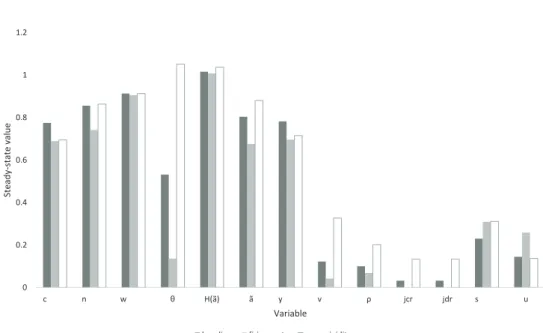
1.3.2 Steady-State Analysis

As a first assessment of the properties of the model, the characteristics of the steady-state are

analysed, in particular the impact in the baseline resulting from the inclusion of firing costs and

full wage rigidity. The general conclusion is that firing costs and wage rigidity have opposite

(49)

values of the main variables of the model stemming from the introduction of firing costs and wage

rigidity is shown in Figure (1.2).

Firing costs limit the reallocation process in the labour market, leading to a lower level of

va-cancies, separations and size of job flows and to a higher percentage of searchers in the labour

force, resulting in a lower level of labour market tightness. While the result regarding job flows

is relatively common in the EPL literature (see Arpaia and Mourre (2012)), the impact on the

un-employment rate is less clear and crucially depends on the way the labour market is modelled. On

the one hand there is less reallocation of labour, given that due to more costly firing, firms avoid

dismissals more strongly than before, but on the other hand, there is also less job creation, given

that the expected value of a job decreases. In the current work, firing costs lead to a reduction

in employment, which confirms the result in Ljungqvist (2002) that the effect of firing costs on

employment is negative in a matching model if there is a relative increase in the share of the match

surplus received by workers, i.e., if firing costs affect the threat point of firms but not the one of

workers. Another effect worth mentioning about the steady-state of the model when compared to

the baseline is the decrease in threshold productivity, resulting from the decrease in the separation

rate, as firms keep workers in employment more time given that it is more costly to fire them.

However the conditional productivity expectationH(˜a)remains almost unchanged. The change

the steady-state level of wages due to the introduction of firing costs is marginal, but negative.

This result is entirely determined by the current calibration, given that a smaller steady-state rate

of searchers would lead wages to increase. In this case, the positive term added to the wage

expres-sion as a result of firing costs, translating an increased bargaining weight obtained by workers, is

overturned by the strong decrease in labour market tightness. The negative impact of firing costs

in employment leads to a decrease in household income and consequently in consumption.

(50)

the number of vacancies, the separation rate and the size of job flows to be higher. As mentioned

in Section 1.2.2, wage rigidity implies to some extent wage compression, given that now all wage

rates, including the one corresponding to the threshold productivity level, depend on the wage

norm. This leads to an increase in the threshold productivity level, and consequently in the

sep-aration rate and job flows (given that job destruction is identical to job creation in steady-state).

However, the average wage rate remains unchanged by definition. With wage flexibility, firms

realize that an increase in treshold productivity implies a corresponding change in wages, thus

par-tially annulling the effect of higher idiosyncratic productivity in profits. With full wage rigidity,

this effect disappears, and therefore new profit opportunities arise. Symmetrically to what happens

with firing costs, the expected value of a job increases, given thata˜increases while the wage rate

is unchanged. This leads to an increase in the number of vacancies posted and consequently in

labour market tightness, and therefore the probability of filling a vacancy (q(θ)) decreases until

the effective cost of a vacancy rises to the new value of a job. The number of searchers increases,

although less than the number of vacancies, reflecting the increase in the separation rate, given

that unemployment remains almost unchanged. Despite the fact that the level of output is almost

unchanged, the steady-state level of consumption decreases, reflecting the cost for the economy of

the additional vacancies posted.

1.3.3 Business Cycle Properties Analysis

Impulse Response Functions

In order to analyze the business cycle properties of the model, its responses to productivity and

monetary shocks where simulated for several possible degrees of wage rigidity and firing costs

(51)

Figure 1.2: Steady-State Comparison

0 0.2 0.4 0.6 0.8 1 1.2

c n w ɽ H(ã) ã y v ʌ jcr jdr s u

S

te

a

d

y

Ͳ

st

a

te

v

a

lu

e

Variable

baseline firingcosts wagerigidity

Legend: The calibration underlying the steady-state values is displayed in Table (1.1). The baseline model does not include firing costs and wages are fully flexible. The firing cost model includes firing costs through the parameterδ= 0.09. The wage rigidity model corresponds to full wage rigidity at the wage normw¯, corresponding to the baseline wage rate.

to the model was therefore simulated using a generalization of Uhlig’s toolkit Matlab code (see

Uhlig (2001) and Uhlig (2006)).

Figures (1.3) and (1.4) show the response of the model to a 1 per cent increase inA, the

non-specific productivity level, and to a 1 per cent increase in money growth, for different levels of

firing costs and degrees of wage rigidity. The figures show that the baseline responses (δ=0 and

γ=1) replicate fairly well those of Krause and Lubik (2007).

Technology shock

As regards the baseline response to a supply side shock, this implies that the amount of goods

produced by each employee increases. Marginal costs decrease due to the unit labour costs

compo-nent of equation (1.34), thus creating incentives for inflation to decrease. Due to the existence of

(52)

remains above steady-state level for some time, increasing the value of a job. This creates

in-centives for firms to expand their labour force, what is achieved both by reducing job destruction

(which implies a decrease in the separation rate and consequently on the threshold productivity

level) and, to a smaller extent, by increasing vacancy creation. The separation channel dominates

the adjustment given that they are costless and have an immediate impact in the employment level.

The increase in vacancies and decrease in the number of searchers drives labour market tightness

upwards, up to a point where the increased real cost of posting vacancies balances the expected

higher profitability of firms (see equation (1.33)). In the period of impact of the shock there is a

temporary increase in separations and a decrease in wages. This short-lived effect results from the

fact that demand does not react immediately to increased supply, due to the sluggish adjustment

of prices.

Monetary shock

In the case of the monetary shock, the increase in the real stock of money balances leads to a

decrease in the real interest rate, and consequently to an increase in demand. Increased demand

leads to an increase in the prices set by intermediate goods firms, although not immediately to the

new desired level due to the presence of adjustment costs. Upon the impact of the shock, given

that the number of employment relationships was determined in the previous period, the only way

firms can adjust their labour force in response to higher demand is by decreasing separations. This

happens in an abrupt and more substantial way than in the case of the productivity shock. This

effect gives rise to a decrease in threshold productivity. The lower number of job searchers drives

labour market tightness upwards, increasing the expected cost of posting a vacancy,( c q(θ)

) . This

effect creates upward pressure on wages and marginal costs, which eliminates the incentives to

post additional vacancies. Moreover, vacancies and job creation actually decrease, given that the

(53)

and rapidly compensated by increasing marginal costs. This response precludes the existence of

a Beveridge Curve as well as the labour market stylized fact of negative correlation between the

business cycle responses of job creation and job destruction rates.

Wage rigidity

As regards the impact of wage rigidity in this framework, Figures (1.3) and (1.4) show that

for a given level of firing costs, wage rigidity amplifies the response of most real variables to

both the productivity and the monetary shock. In a flexible wage setting, wage adjustments would

limit the real effects of the shocks in the labour market by restraining the increase in the expected

value of a job for the firm. This counterbalancing effect disappears with wage rigidity, which

leads to increased incentives to hiring and vacancy posting and consequently to stronger effects in

employment and production. In the case of the monetary shock, the additional posting of vacancies

actually leads, for a large enough degree of wage rigidity, to a change in the sign of the response

of vacancies, which shifts from negative to positive. This apparently creates a Beveridge curve

relationship that was absent in the baseline, as pointed out by Krause and Lubik (2007). However,

a very high degree of wage rigidity is required for this feature to emerge. Moreover, the impact

of wage rigidity on the inflation response is relatively limited, reflecting the almost unchanged

response of marginal costs.

Firing costs

In a wage flexibility scenario, increasing firing costs makes the threshold productivity level

less sensitive to cyclical fluctuations, leading to a more muted response of the separation rate in

the case of both shocks.8 _{Therefore, prices gain importance as an instrument available for firms}

8_{Despite the fact that the threshold productivity level becomes more sensitive to the job finding rate}

(θq(θ)) as the level of firing costs increases (see equation (1.50)), the steady-state level ofa˜also decreases.

(54)

to react to increased supply or demand. Given that, prices fall more intensely than in the baseline

in response to a productivity shock, leading to an amplification of the size and persistence of the

response of real variables, in particular labour market tightness, but also output and consumption.

In the case of the monetary shock, the effect is similar although of opposite sign: prices react more

strongly upwards and this increase is largely concentrated in the period of impact of the shock. As

a result, the impact of the shock on real variables becomes more muted.

Given that the response of the separation rate is more moderate for both shocks, vacancies

as-sume an increasing role for labour market adjustment. In the case of the monetary shock, for a large

enough size of the firing costs this leads the response of vacancies to turn from positive to negative.

As regards job flows, the response of the job creation and destruction rates is now smaller, which

confirms the results of several studies regarding EPL (see Arpaia and Mourre (2012)). The

im-pulse response functions for these variables, as well as for unemployment, expressed in percentage

points, are presented in Figures (1.3) and (1.4).

Interaction between firing costs and wage rigidity

As a result of the above analysis, the interaction of firing costs and wage rigidity amplifies

the impact of productivity shocks on real variables, given that these features have complementary

effects as regards the strength and persistence of responses. On the contrary, in the case of monetary

shocks, firing costs and wage rigidity act as substitute forces, given that wage rigidity increases the

response of the expected value of a job to a shock, while the introduction of firing costs decreases

it. The effect of firing costs seems to dominate until the degree of wage rigidity is above 50 per

cent. For higher degrees of wage rigidity, the response of output and inflation becomes largely

unaffected by the level of firing costs. This may be related to the fact that because the wage is

Firing and training costs and labour market segmentation