Monte Carlo Simulation of Grain Growth
Paulo Blikstein, André Paulo Tschiptschin
Depto. de Eng. Metalúrgica e de Materiais, Escola Politécnica da Universidade de São Paulo Av. Prof. Mello Moraes, 2463 São Paulo - SP, Brazil
Received: August 15, 1998; Revised: March 30, 1999
Understanding and predicting grain growth in Metallurgy is meaningful. Monte Carlo methods have been used in computer simulations in many different fields of knowledge. Grain growth simulation using this method is especially attractive as
• the statistical behavior of the atoms is properly reproduced;
• microstructural evolution depends only on the real topology of the grains and not on any kind of geometric simplification.
Computer simulation has the advantage of allowing the user to visualize graphically the procedures, even dynamically and in three dimensions.
Single-phase alloy grain growth simulation was carried out by calculating the free energy of each atom in the lattice (with its present crystallographic orientation) and comparing this value to another one calculated with a different random orientation. When the resulting free energy is lower or equal to the initial value, the new orientation replaces the former. The measure of time is the Monte Carlo Step (MCS), which involves a series of trials throughout the lattice. A very close relationship between experimental and theoretical values for the grain growth exponent (n) was observed.
Keywords:Monte Carlo simulation, grain growth, physical metallurgy, scientific visuali-zation
1. Introduction
Grain size is a very important characteristic for evalu-ating the properties of the materials, especially when we need to balance different ones. It is, in fact, one of the most important issues in the control of microstructure1. As a result, this phenomenon is exhaustively studied in Metal-lurgy.
Usually this kind of study is made through careful analysis and comparison of microstructures, often with the help of image analysis software. Recently, as the process-ing power of computers increased a new and promisprocess-ing approach has been made possible: computer simulation of grain growth.
Srolovitz et al.2,3 proposed the most widely known and employed theory for computer modeling and simulation of grain growth, using the Monte Carlo method. There is a very interesting relationship between the conceptual basis of the Monte Carlo method and the physical characteristics of grain growth. As far as both rely very much on statistics and randomness, the method seems to represent the phe-nomenon very well.
2. Grain Boundary Migration
During grain growth the boundary equilibrium is reached when the angles among them follow the equation:
γ1 − 2
sin α1
= γ2 − 3 sin α2
= γ1− 3
sin α3
(1)
where αn are the angles between boundaries and γn-m are
the specific surface energies. In a single-phase alloy, considering a 2D simplified anisotropic structure, the equilibrium angle is 120°.
Burke4 proposed that the rate of boundary migration would be inversely proportional to the average curvature radius:
R = k tn (2)
where R is the grain diameter, t is the time and k is a constant that varies exponentially with temperature. The maximum value of the exponent n (rarely observed experimentally) is 0.50.
Equation 2, however, describes only an average growth. It cannot predict, for instance, different growth rates for the
a
e-mail: [email protected]
b
different grain size classes present in the microstructure. As a result, we conclude that there are very important issues that are simply not possible to evaluate without computer simulation. As mentioned by Srolovitz et al.:
“While it is generally observed that large grains grow and small grains shrink, instances where the opposite is true can be found. This suggests that knowledge of the instan-taneous absolute or normalized grain sizes is not sufficient to predict the evolution, or even the direction of evolution, of individual grains. [...] The results indicate the validity of a random walk description of grain growth kinetics for large grains, and curvature driven kinetics for small grains.”3
Computer simulation of grain growth plays an impor-tant role in understanding it. The goal is not simply to confirm the conventional theory, but to investigate new issues.
3. Description of the Method
The concept behind the Monte Carlo method in grain growth simulation is both simple and fascinating: its only basis is the thermodynamic of atomic interactions. There are no other experimental or theoretical inferences, nor mathematical approximations.
The first step is to represent the material as a 2D or 3D matrix, in which each site corresponds to a surface or volume element. The content of each element represents its crystallographic orientation. Contiguous regions (contain-ing the same “number”) represent the grains as shown in Fig. 1. The grain boundaries are fictitious surfaces that separate volumes with different orientations.
After choosing the kind of matrix and filling it with an initial random content, the simulation itself begins. These are the four main steps of the algorithm:
a) Calculation of the free energy of an element of the matrix (Gi) with its present crystallographic orientation
(Qi) based on its neighborhood.
b) Random choice of a new crystallographic orientation for that element (Qf).
c) New calculation of the free energy of the same element (Gf), but with the new crystallographic orientation
(Qf).
d) Comparison of the two values (Gf-Gi). The
orienta-tion that minimizes the energy is chosen.
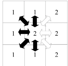
These four steps are repeated millions of times in ran-dom positions of the matrix. The overall result is a micro-scopic simulation of the free energy decay in the system, which is actually the main impelling force for grain growth. Figures 2 and 3 show schematically the four main steps applied to one element of the matrix. Figure 4 shows an example of energy calculation at a stable triple point where any reorientation attempt would lead to the same free energy value.
The Hamiltonian that describes the interaction among the closest neighbors, which represents the grain boundary energy, is:
H =− J
∑
nn
(δSiSj−1) (3)
where Si is one of the Q possible orientations in the i element of the matrix and δab is the Kronecker-delta, which
is 1 when the two elements are equal and 0 otherwise. As a result, neighbors with a different orientation contribute J to the system energy and 0 when equal. The transition probability W is:
Figure 1. The grain structure represented by a 2D square matrix.
Figure 2. Calculation of the free energy of an element of the matrix (Qi
exp (− ∆G
kb T)
→∆G > 0
1 →∆G ≤0 (4)
where ∆G is the change in free energy due to the orientation alteration, kb is the Boltzman constant and T is the temperature. Thus the speed of the moving segment is given by:
vi= C [1 − exp(−∆ Gi
kb T)] (5)
where C is the boundary mobility.
4. Evolutions of the Classical Method
At first sight, the algorithm describes accurately the physical phenomena. Nevertheless, some authors noticed problems: nucleation of an “artificial” grain inside others
(which does not occur experimentally) and values of n below 0.50 (the theoretical value of the grain growth expo-nent). Radhakrishnan e Zacharia6 proposed a new algo-rithm that would at one time eliminate artificial nucleation, raise the value of n and decrease significantly the comput-ing time required for the simulation.
The new algorithm proposes that the new orientation to be “evaluated” in each matrix element would no more be chosen among all the possible ones (Q-1), but only among those that surround each element. In other words, if an element has in its surroundings grains with orientations 3, 6, 13 and 15, the new one will be chosen only among these four values.
This was the algorithm used in our experiments, also called “cellular automata”.
5. Experimental
The software was developed using a C++ compiler. The program was executed in a Pentium-Pro 233 MHz machine with 128 MB of RAM. The machine showed up to be very satisfactory in terms of speed and reliability for 2D simu-lations.
The visualization of the matrix was carried out through conventional image processing software. The 3D visuali-zation (which is still being improved) was done in a Silicon Graphics workstation running the AVS visualization pack-age.
6. Results in a 2D Square Lattice
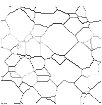
The experiments took place in a 200 x 200 matrix. The dimensional evolution of the grains was measured by evaluating the total amount of interface in the system. In Fig. 5 we can observe the microstructure after some simu-lation steps.
The first important issue to be analyzed is the geometry (square or triangular) of the matrix to be used. Srolovitz et al.1 analyzed this problem and reached the conclusion that the results were equivalent, provided higher temperatures were used in the simulations with square matrix. This is due to the fact that in this kind of discretization, a perfect 120° angle between boundaries in not possible. In the triangular lattice, the temperature can be set to T = 0 as its geometric nature can represent with more accuracy the triple points and grain boundaries. Temperature, in all these Monte Carlo simulations, is not directly related to “real” tempera-ture. It is just a correction factor for the different charac-teristics of the lattices. Some authors introduced “real” temperature gradients in the simulation model by changing boundary mobility along the matrix7.
The second important issue is the maximum number of possible orientations (Q). The first experiments by Srolovitz et al.2 employed values from 4 to 64, while Radhakrishnan6 proposed N2, where N is the dimension of the matrix (in a 200 x 200 matrix, Q = 2002 = 40,000), as W =
{
Figure 3. After an attempt of reorientation To Qf = 1, the free energy is
reduced to Gf = 3. hence the NEW orientation should be maintained.
to avoid artificial grain coalescence. We ran nine series of simulations, with values of Q from 8 to 30,000. The results are shown in Fig. 6. It is clearly noticeable that the value of Q alters the kinetics of grain growth. For the lowest value (8) the grain growth exponent is the highest (0.54), prob-ably due to artificial grain coalescence. However, much higher Q values (256, 512, 1024, 30000) did not improve significantly the results, which were very similar to those obtained in the simulations with Q = 64 or Q = 128. Srolovitz et al.2 performed a similar experiment and con-cluded that for Q > 30 the simulation becomes Q-inde-pendent. Based on these results a Q value of 128 was chosen for the subsequent experiments.
After these initial experiments, we proceeded to grain growth investigation itself. The conventional algorithm proposes that the new orientation should be chosen at random among all possible orientations (Q-1). Experiments obtained with this algorithm2,3,6 reached values for the grain growth exponent n still far from the theoretical value
(0.50). Radhakrishnan demonstrated that the kinetics of the conventional method would lead to a significantly slower microstructural evolution, and proposed a new one, which is widely employed nowadays.
To investigate this issue, we ran two series of simula-tions, with the old and new algorithm. Fig. 7 shows the results. There was a clear difference between the two simulations, both in the growth kinetics and the final mi-crostructure. Using the old algorithm, we reached values for n within the 0.35 - 0.39 range. Employing the new algorithm, the values were in the 0.48 - 0.51 range, much closer to the theoretical 0.50.
After averaging a series of simulations with the new algorithm, in a square matrix of 200 x 200, the value of 0.509 was reached. We also proceeded a careful statistical analysis of the local slopes of the grain growth curve. As expected, the histogram shown in Fig. 8 revealedthat most of the local slopes were within the 0.40 - 0.60 range. As the simulations relies very much on random numbers, it is not surprising that there are negative slopes (-0.60) as well as much higher ones (+1.60). The average, however, was very close to what was expected (0.50).
In the log x log scale of the graph in Fig. 9 it is possible to notice the linear behavior of the average curve. In very long simulations (> 50,000 MCS) we noticed that the system reaches stability, with a very small number of grains. Reaching a sufficiently large size, their growth slows down, as most of the boundaries become flat (in a square matrix).The values of n found in the simulation are in very good agreement with the experiments of various
Figure 5. The microstructure after editing in image processing software.
Figure 6. Grain growth behavior for increasing q values.
authors, as Srolovitz et al.2,3, Zacaria6 and Mehnert8,9. That demonstrates the validity of the software elaborated for the simulation and the model adopted.
The method discussed in this paper can be used in Metallurgy to study real-world problems, as the micro-structure evolution during the welding process10 and grain growth pinning in advanced materials.
7. Conclusion
The computational simulation demonstrated that the grain growth phenomenon, although complex, could be modeled in a very elementary way. The correct value of n, found in our experiments, indicate that there is a very close relationship between the model and the theoretical descrip-tion of grain growth.
References
1. Liu, Y.; Baudin, T.; Penelle P. “Simulation of normal grain growth by cellular automata”. Scripta Materi-alia, v. 32, n. 11, p. 1679-1683, 1996.
2. Anderson, M.P.; Srolovitz, D.J.; Grest, G.S.; Sahni P.S. “Computer simulation of grain growth” – I. Ki-netics”, Acta Metallurgica, n. 32, p. 783-792, 1984. 3. Anderson, M.P.; Srolovitz, D.J.; Grest, G.S.; Sahni,
P.S. “Computer simulation of grain growth - II. Grain size distribution, topology and local dynamics”, Acta Metallurgica n. 32, p. 793-801, 1984.
4. Burke, J.E. Trans. Am. Inst. Min. Engrs, n. 180, p. 73, 1949.
5. Saito, Y.; Enomoto, M. “Monte Carlo simulation of grain growth”. ISIJ International, v. 32, n. 3, p. 267-274 1992,.
6. Radhakrishnan, B.; Zacharia, T. “Simulation of cur-vature-driven grain growth by using a modified Monte Carlo algorithm”. Metall. And Mater. Trans. A, n. 26A, , p. 167, 1995.
7. Miodownik, M.A. Sandia National Labs, personal communication, 1998.
8. Mehnert, K.; Klimanek. P. “Monte Carlo simulation of grain growth in textured metals”. Scripta Materi-alia, v. 30, n. 6, p. 699-704, 1996.
9. Mehnert, K.; Klimanek, P. “Grain growth in metals with strong textures: three-dimensional Monte Carlo simulations”. Computational Materials Science, 1997.
10. Fye, Richard. Sandia National Labs, personal com-munication, 1998.
Figure 8. Histogram of the local slopes.