*e-mail: [email protected]
1. Introduction
The understanding and modeling of dendritic growth has remained a central theme of solidiication research for many years. Understanding the solidiication process is of great importance because the resulting microstructures determine the properties of the material. Although there have been signiicant developments in understanding dendritic structures in the past decades, our knowledge of the dendritic growth is based on experiments and idealized theoretical models. On the other hand, phase-ield models are known to be very powerful in describing non-equilibrium dendritic evolution. They are very eficient because, in the numerical treatment based on them, all the governing equations are written for the whole domain without distinguishing the interface from the solid and liquid phases. Furthermore, direct tracking of the interface position is not needed during numerical simulation of the solidiication process. The phase-ield models were developed mainly for studying solidiication of pure materials1, being then extended to the solidiication of binary2, ternary3, and quaternary in Salvino et al.4 alloys.
Recently, Xu et al.5 used phase-ield models focused on pure materials. Their paper presented a detailed numerical method and algorithm for solving two-dimensional (2-D) phase-ield model. Comparison between the fully-coupled and sequential techniques showed that CPU time of the second approach is approximate 10% greater than that of the irst one. However, the sequential method is chosen for computations in order to reduce storage requirements as much as possible. The authors found that the numerical results capture well the complex physics of the solidiication problem. Consistent with physical reality, the computed critical radius indicates existence of a critical value for a nucleus to grow in the phase ield simulation. Moreover, the critical radius decreases linearly with increasing Stefan number, which means that, if the Stefan number is large enough, solidiication always takes place, no matter what the initial conditions are. In addition, they studied dendrite shapes at different degrees of supercooling; the results are in agreement with the experimental results.
Moelans et al.6 published a paper presenting an introduction to phase-ield models and an overview of their possibilities. Amongst those, as listed by the authors,
Simulation of the Microstructural Evolution of Pure Material and Alloys in an
Undercooled Melts via Phase-ield Method and Adaptive Computational Domain
Alexandre Furtado Ferreiraa*, Ivaldo Leão Ferreiraa,
Janaan Pereira da Cunhaa, Ingrid Meirelles Salvinoa
aUniversidade Federal Fluminense – UFF, Volta Redonda, Rio de Janeiro, Brazil
Received: April 29, 2014; Revised: April 28, 2015
The phase-ield methods were developed mainly for studying solidiication of pure materials, being then extended to the solidiication of alloys. In spite of phase-ield models being suitable for simulating solidiication processes, they suffer from low computational eficiency. In this study, we present a numerical technique for the improvement of computational eficiency for computation of microstructural evolution for both pure metal and binary alloy during solidiication process. The goal of this technique is for the computational domain to grow around the microstructure and ixed the grid spacing, while solidiication advances into the liquid region. In the numerical simulations of pure metal, the phase-ield model is based on the energy and phase equations, while, for binary alloy, the said model is based on the concentration and phase equations. Since the thermal diffusivity in the energy equation is much larger than the diffusivity term in phase equation in pure metal system, about twenty eight times the difference between them. The computational domain growth around the microstructure is controlled according with the thermal diffusivity for pure material in the liquid region. In the numerical simulation of dendritic evolution of Fe-C alloy, the idea is similar, i.e., the solute diffusivity in concentration equation is larger than the diffusivity term in phase equation in the liquid region, in this case eleven times the difference in Fe-C alloy system. The computational domain growth is controlled via solute diffusivity in the liquid region. Hence, phase-ield model is proposed with an adaptive computational domain for eficient computational simulation of the dendritic growth in a system for both pure metal and binary alloy. The technique enables us to reduce by about an order of magnitude the run time for simulation of the solidiication process. The results showed that the microstructure with well-developed secondary arms can be obtained with low computation time.
was the simulation of solidiication processes, precipitate growth and, more recently, an application to solid-state phase transformations like the austenite-to-ferrite transformation in steels, dislocation dynamics, as well as crack nucleation and propagation. Achievements are expanding rapidly, due to improved modeling and implementation techniques and growing computer capacity.
From a somewhat more theoretical standpoint, it should be noted that the interface morphology of the solidiication front calculated by phase-ield models reproduces the known patterns of a dendrite structure. The state of the domain is represented by the distribution of a single variable known as the order parameter, ϕ, or phase-ield variable. In this study, the solid state is represented by ϕ = +1, while, in the liquid region, ϕ = 0. The region in which ϕ changes progressively from +1 to 0 is deined as the solid/liquid interface. In spite of phase-ield models being suitable for simulating solidiication processes, as mentioned by Moelans et al.6, they suffer from low computational eficiency. For example, for computation of a dendrite with side-branches, the computational domain should be discretized into one million points. Thus, the computational stability condition in an explicit inite scheme can be guaranteed only with a very small time step. Xu et al.5 show a sequential method to reduce required storage during the calculations of the solidiication process. In this study, on the other hand, we present a numerical technique for the improvement of computational eficiency for computation of dendritic evolution in solidiication processes for both pure material (Ni) and binary alloy (Fe-C). In both cases presented in this article, at the start of the solidiication process, there is a solid nucleus placed in the very small computational domain. The goal of this technique is for the computational domain to grow around the dendrite and ixed the grid spacing, while solidiication advances into the liquid. The transient response of the phase equation is controlled by the product
M.ε2. This parameter acts in the phase-ield model similarly
to the thermal diffusivity (D) in the energy transport equation. Since the thermal diffusivity is much larger than the product
M.ε2, in pure metal system, for example twenty eight times
difference in pure material system, the effect of heat transfer irst occurs in the pure metal system. This way, the growth around the dendrite is controlled according with the thermal diffusivity (D) in liquid region. For numerical simulation of the dendritic evolution of binary alloy (Fe-C), the idea is similar to the pure metal (Ni). In other words, the solute diffusivity in liquid region (DL) is larger than said product M-ε(θ)2, so
the growth of the domain around the dendrite is controlled via solute diffusivity in liquid. The numerical technique for both cases pure metal (Ni) and alloy (Fe-C) enables us to reduce the run time in simulation of dendritic evolution during solidiication process.
2. Phase-field Modeling
2.1. Phase-ield modeling for pure materials
The phase-ield model is based on the simultaneous solution of energy and phase equations for pure materials. Phase-ield modeling assumes the growth of seeds in the liquid phase. According to this hypothesis, there are three regions to be considered: the solid nucleus, the liquid phase
and the solid/liquid interface. The state of the entire domain is represented by the distribution of a single variable known as the order parameter,ϕ, or phase-ield variable. The region in which ϕ changes from 1 to 0 is deined as the solid/liquid interface. The time evolution equation of the phase-ield ϕ is described by1:
(1)
where M is deined as the solid/liquid interface mobility, the
angle θ is given by the orientation of a vector perpendicular to the solid/liquid interface, e.g., ∇ϕ. ΔH is the latent heat and Tm the melting temperature. The function g’(ϕ) that multiplies w determines the distribution of the excess free-energy at the interface. h(ϕ) is a function that satisies the condition h’(0) = h’(1) = 0. As in reference Moelans et al.6, we chose
(2)
(3)
The method most widely used to include anisotropy for a two-dimensional calculation is to assume that ε in Equation 1 depends on θ, the orientation of the normal to the interface with respect to the x-axis:
(4)
where δε is the anisotropy constant. The value of j controls the number of preferential directions of the material’s anisotropy, equaling 0 for the isotropic cases, 4 for anisotropy of 4 directions, and so on. The constant θo is the interface
orientation with respect to the maximum anisotropy, while ε and w are parameters associated with the interfacial energy (σ)
and interface thickness (λ), as proposed by Boettinger et al.7:
(5)
(6)
For the interface mobility, we follow references Ferreira et al.1 and Boettinger et al.7:
(7)
where μ is the linear interface kinetic coeficient. The phase-field model particularized for a pure material, subjected to a nonuniform thermal ield, includes an energy transport equation:
(8)
positive for solidiication, ρ is the material´s density, assumed to be the same both solid and liquid phase, and Cp is the speciic heat.
2.2. Phase-ield modeling for binary alloy
The phase-ield equation for simulates the solidiication process for binary alloy is described by2:
(9)
The evolution of the solid nucleus with time (∂ϕ⁄∂t) is assumed to be proportional to the variation of the free-energy functional with respect to the order parameter, ϕ. The terms of the phase equation are derived from this free-energy functional, which must decrease during any solidiication process, as indicated in the article by Salvino et al.4. The last product on the right-hand side translates the driving force behind the solidiication process. Here, R is the gas constant and Vm, the molar volume. The arguments to the natural logarithms, and , are, respectively, the equilibrium concentrations of carbon in the solid and liquid region. Their respective ordinary concentrations in the liquid and solid regions are denoted, by the pairs CL and CS.
As proposed by Ode et al.2, concentrations of carbon in both regions is calculated with the solute transport equation, numbered (10),
(10)
In this equation, D(ϕ) is the carbon diffusivity in the solid and liquid regions. The model used here takes into account solute diffusivity in the liquid and interface regions.
The model parameters ε and w for binary alloys are
calculated in the same way as proposed by Boettinger et al.7, Equations 5 and 6. From Salvino et al.4, the phase-equation mobility for binary alloys, M, is computed as
(11)
where the is obtained from
(12)
In Equations 11 and 12, L and S stand for liquid and solid, respectively.
3. Numerical Simulation
To simulate growth of an asymmetrical dendrite of pure materials and binary alloys, it is necessary to introduce a noise term in the right-hand side of the phase-ield equations. A usual expression for this noise, as indicated by Ferreira et al.1, is
(13)
where r is a random number between −1 and +1. The
″a″ parameter is the noise amplitude. Maximum noise
corresponds to ϕ = 0.5, at the center of the interface, whereas at ϕ = 0 (liquid region) and ϕ= +1 (solid region) there occurs no noise. That is to say, noise is generated at the interface.
Equations 1, 8, 9 and 10 were solved by an explicit inite-difference method, with a mesh suficiently reined to describe details of the dendrites. Performing the computations with a numerical grid of 200×200 points with parameters determined in the previous section and the physical properties of nickel, it was not feasible to obtain a dendrite with developed secondary arms, due to the small computation domain. Dendrites with fully developed side branches necessitate a computational domain with several million points. However, computation with such a large computational domain is restricted not only by the computational eficiency, but also by memory size. In the present study, we develop a numerical technique in order to improve eficiency. The idea was originally proposed for simulating the dendrite growth from an undercooled pure melt and has been extended to solidiication of binary alloy. In pure metal case (Ni), the thermal diffusivity, in Equation 8, is much larger than the product M-ε (θ )2, in Equation
1, for example about twenty eight times difference in pure material system. Therefore, irst to occur is the effect of the heat transfer, then phase change during simulation of solidiication process. A greater value of D (Equation 8, for pure materials) forces the thermal front to be always ahead of the solidiication interface. Hence, there is always a thermal gradient ahead of the solidiication front. In this study for solidiication of pure materials, the thermal boundary layer is deined as a region with
(14)
where T0 is a given initial undercooled temperature. If the condition T(I,J) > T0 + 1.1 at (I,J) in the square region is satisied, the adaptive computational domain grows around the dendrite. Whenever the condition is satisied, new temperature T(I,J) and phase ϕ(I,J) at the current time step are calculated from the explicit inite-difference method from the values in previous steps, while the computational domain grows one unit of points on the x-y directions. If the condition just stated is not satisied, the computational domain does not grow. The new temperature T(I,J) and phase ϕ(I,J) are then calculated from the values in previous steps for a small-size domain. In the simulation of binary alloy (Fe-C) solidiication, the idea is similar to the pure metal (Ni). In binary alloy case, the phase-ield model is based on the phase and concentration equations. The phase equation includes the product M-ε (θ)2, and D(ϕ) is
solute diffusivity in liquid phase (DL) (Equation 10) is
larger than the product M-ε (θ)2 (Equation 9), about eleven
times is the difference between them. Hence, irst to occur is the concentration change, then the phase change during simulation of solidiication in binary alloy system. In other words, during solidiication, the solutes are rejected into the liquid phase, which then becomes rich in solute just ahead of the interface. The ahead of the interface there is a thickness of the diffusion boundary layer in the liquid due the high mobility of solute in said region. As mobility solute is greater as compared to that front solidiication, it forces the gradient concentration in liquid to be always ahead of the solidiication interface. In the solidiication of binary alloys, the diffusion boundary layer is deined as
(15)
where C0 is a given initial concentration. If the condition is satisied C(I,J) > C0 + 1×10
–3, the adaptive domain grows
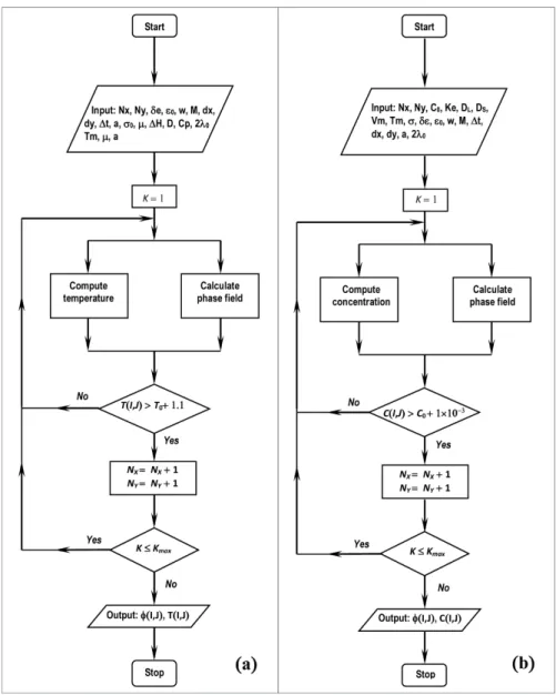
around the binary alloy dendrite; otherwise, it does not grow. The block diagram in Figure 1 shows the low of information in the numerical program for both pure materials (Figure 1a) and binary alloy (Figure 1b).
The calculations were performed on an Intel 2 Quad processor, with 1.38GB RAM. In this study, in the initial stage of solidiication the computational domain used to calculate dendrite evolution is rather small, about 200 × 200 points. Both phase-ield models presented in this article, one with an adaptive computation domain and one with a computation domain of ixed size, were constructed with the same grid spacing (dx = dy = 2 × 10⁻⁸m). The difference is in the number of nodes of the computational domain. In the irst model, the computational domain is very small in the initial steps of the computation; consequently the computational eficiency is improved and the memory size requirement is reduced. In the second model with a computation domain of ixed size, in the initial steps of the computation the computational domain
is very large, thereby reducing computational eficiency and the memory size requirement is increased.
The phase, energy and concentration equations were solved in a computational domain divided into square grids of I × J, with a grid spacing of dx = dy not only for the
thermal ield, but also for calculation of the phase ield and concentration. The thermal ield T(I,J ), phase-ield ϕ(I,J )
and concentration C(I,J) at each point in the grid (I,J) are known from the previous step, by the explicit inite-difference. For each point I,J in the grid, a real value ϕ(I,J), describes the phase state of the grid, is assigned ϕ(I,J) = 0 to indicate the grid in the liquid state and ϕ(I,J) = +1 for the solid state. The ensemble of all grid points with 0.001 < ϕ(I,J ) < 0.999 is taken to represents the interface region.
4. Results and Discussion
In order to test the computational eficiency of our numerical technique, we compared the computer run time for the calculation of dendritic growth in undercooled melts using a phase-ield model with and without an adaptive computational domain. We analyzed the computational eficiency for both cases pure material (Ni) and binary
alloy (Fe-C).
4.1. Phase-ield simulation of dendritic
solidiication for pure material
The parameters and properties adopted in this study for pure materials (Ni) are summarized in Tables 1 and 2, respectively. The phase-ield mobility (M) for pure metal is calculated by Equation 7.
To exhibit the similarities between the dendrites of nickel calculated in the present paper and those described in the literature, we introduce Figure 2. In that igure, both pictures display: a) the secondary arms; b) the secondary arm increase with distance behind the primary dendrite tip; c) the asymmetry of the side branch found in the secondary arms; and d) the secondary arms growth rigorously perpendicular to the primary arm.
Figure 3 shows temperature proiles and the phase-ield variable across solid, interface and liquid regions. In this simulation, the solid/liquid interface advances into the liquid region. The transient response of phase-ield equations is controlled by the product M-ε (θ)2, in Equation 1. This
parameters act in the phase-ield model similarly to the thermal diffusivity D in the thermal energy Equation 8. As Kim et al.8 pointed out, in the formation of a dendritic morphology in pure metals, it is important that the thermal diffusivity becomes greater than its similar term, M-ε (θ)2.
This can be explained by analyzing Figure 3. The greater value of D forced the thermal front to be always ahead of the solidiication interface. Hence, there was always a thermal gradient ahead of interface. In pure metal case (Ni), the thermal diffusivity (D), in Equation 8, is much larger than the product M-ε (θ)2, in Equation 1, for example about
twenty eight times difference in pure material system. On the other words, irst of all occur the temperature change, and then the liquid becomes solid region. Hence, the present paper is based in that approach, i.e., if the temperature change occurs, the adaptive computational domain grows
Table 1. Model parameters (Ni).
Anisotropy constant, δε 0.025
Coefficient of phase-field gradient energy term, εo
2.01×10− 4 (J/m)1/2
Free energy factor, w 0.61×10 8 J/m3
Phase-ield mobility, M 13.47m3/sec⋅J
Grid spacing, dx 2×10− 8 m
Grid spacing, dy 2×10− 8 m
Time step, Δt 1×10− 12 sec
Noise amplitude factor, a 0.025
Table 2. Material properties of Ni8.
Interface energy,σo 0.37 J/m
2
Kinetic coeficient at interface, μ 2 m/s. K
Melting temperature, TM 1728 K
Latent heat, ΔH 2.35×10 9 J/m3
Thermal diffusivity, D 1.55×10 – 5 m2/s
Speciic heat, CP 5.42×10 6 J/m3. K
Interface width, 2λo 8×10
– 8 m
Figure 2. (a) Present calculation and (b) dendrite found in the literature, Prates11.
Figure 3. Temperature and phase-ield variable proiles across solid,
around the dendrite; otherwise, the computational domain size is kept constant.
In order to test the computational eficiency of our numerical technique, we compared the computer run time for calculation of dendritic growth in undercooled melts using a phase-ield model with and without an adaptive computational domain. Figure 4 shows the dendrite growth obtained by the phase-ield model with the adaptive computational domain for different solidiication times and domain sizes.
Figures 4a-d shows the development of the adaptive computational domain for dendritic growth. In Figure 4a, the dendrite started to grow from a nucleus added at the center of the computational domain with 85×85 points, solidiication time being equal to 4.47×10⁻⁹sec, insuficient
for growth of primary and secondary arms. In Figure 4b, the numerical grid (205×205) is larger than that of Figure 4a (85×85), due to the dendrite tip advancing into supercooled liquid during the solidiication process. In Figure 4b, one observes only primary arms, with no side branching, for a solidiication time of 3.62×10⁻⁸sec. In Figure 4c, the
time for solidiication (9.35×10⁻⁸sec) is suficient for the
growth of secondary arms. Finally, in Figure 4d, the time for solidiication is 1.50×10⁻⁷sec and the numerical grid
comprises 605×605 points. Here, it is possible to observe well-developed secondary arms away from the dendrite tip, while small side branches compete with each other shortly behind the dendrite tip. The asymmetry in the side branches is evinced in Figures 4c, d. This follows from the thermal ield distribution. Again, side branching prefers the direction
of latent heat release. In all of Figure 4, computational convergence is optimized through adoption of a small computational domain around the dendrite.
Figure 5 shows variation of computer run time (in seconds) as a function of primary dendrite length (in units of domain size). There, the open and solid circles are for the adaptive computational domain and a computational domain of ixed size, respectively. One can see that, with the adaptive computational domain, the run time required to reach a given primary dendrite growth is about a tenth of that with the computational domain of ixed size. Computational eficiency is guaranteed by using an adaptive computational domain for phase ield and thermal calculation, in pure metal system. Because the computational domain is small at the beginning of the calculations, convergence is optimized.
Using the phase-field model with an adaptive computational domain for simulation of the solidiication process, the calculation of dendritic growth is carried through with a computational domain suficiently small for the phase ield and thermal calculations. Increasing the primary dendrite length, one inds that the run-time versus primary-dendrite-length plot will tend to exhibit an exponential-like behavior.
4.2. Phase-ield simulation of dendritic
solidiication for binary alloy
Table 3 presents the physical properties of the binary alloy used in the computations that follow. The parameters used in the phase-ield model obtained of physical properties of the material were derived from Equations 5, 6, and 11.
Figure 4. Development of the adaptive computational domain for dendritic growth. The numerical grids and solidiication times are: (a) 85×85
Table 4 presents these parameters. The phase-ield mobility (M) for binary alloy (Fe-C) é calculated by Equations
11 and 12. The boundary condition adopted for the phase-ield model (ϕ) in this work is a zero-lux condition.
The Figure 6 shows the dendritic morphology obtained by both the phase-ield model with adaptive computational domain (Figure 6a) and ixed domain (Figure 6b); one can see excellent agreement between the two cases. Figure 6 depicts the simulation of a Fe-C alloy calculated with a regular grid. In this simulation, a dendrite is presented with secondary arms. The secondary arms increase with the distance behind the primary dendrite tip. This was observed in experiments on dendritic growth in undercooled melts. The asymmetry in the side branches of the primary arms
observed in both Figure 6a-b is due to a noise source added to the phase-ield equation.
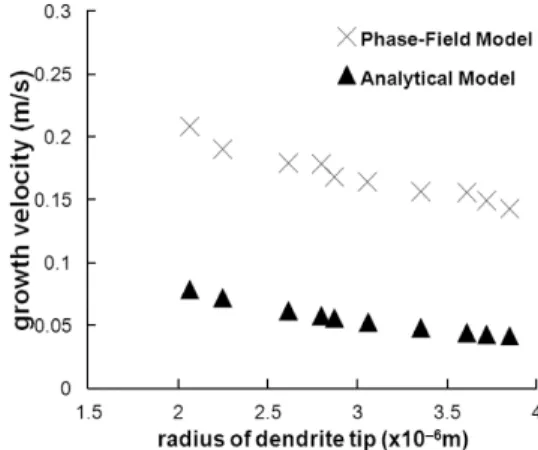
In order to show the applicability of the phase-ield model with adaptive computational domain, the inluence of dendrite tip radius on the growth velocity is showed. The relationships between growth velocity and dendrite tip radius for a Fe-C alloy are shown in Figure 7. Data calculated by an analytical model, proposed by Stenanescu9, were plotted alongside for comparison. We can see that phase-ield-based results lie above those obtained with analytical model proposed by Stefanescu.9 This may happen due to the evolution of the solid phase with time (Equation 9) is assumed to be dependent of the source term. This, in turn, depends of both concentrations in the solid and liquid region and temperature. The Stefanescu’s model, on the other hand, takes into account tip radius and concentrations in the liquid region. One can see in Figure 7 that increasing the radius of dendrite tip inluences the reduction of the dendritic growth velocity. The numerical results for the tip velocity are consistent with experimental conclusion, Altundas and Caginalp10, and compatible with the literature9, 11 that tip velocity will decrease for larger radii.
Figure 8 exhibits the results of the carbon concentrations; we compare the results of a one-dimensional phase-ield calculation with the predictions by Scheil’s equation and by the Clyne-Kurz equation. The initial temperature of the computational domain is 1780K. For the calculations of carbon concentration, we assumed an isothermal
Table 3. Physical properties of the binary alloy analyzed.4
Property C Fe
Initial concentration, C0 6.93.×.10.−.3 mol % —
Partition coeficient, KE 0.17171 —
Slope of liquids line, ME 1772.77 K/mol —
Diffusivity in liquid phase, DL 2.0
.×.10.−.8 m2/s — Diffusivity in solid phase, DS 6.0.×.10.−.9 m2/s —
Molar volume, VM — 7.7
.×.10.−.6 m3/mol
Melting temperature, TM — 1811 K
Interface energy, σ — 0.204 J/m2
Table 4. Computational parameters.
Anisotropy constant, δε 0.05
Coeficient of phase-ield gradient energy
term, ε0 1.05
.×.10.−.4
(J/m) 1/2
Free energy factor, w 6. 73.×.107 J/m3
Phase-ield mobility, M 0.166 m3/s.J
Time step, Δt 1.0.×.10.−.8 s
Grid spacing, dx 2.0.×.10.−.8 m
Grid spacing, dy 2.0.×.10.−.8 m
Noise amplitude factor, a 0.025
Figure 5. Variation of computer run time as a function of primary
dendrite length, in units of points.
solidiication process. In the calculations, no anisotropy was imposed. The calculated carbon proile agrees better with the Clyne-Kurz equation than with Scheil’s equation, when the solid fraction is above 0.5, as shown in Figures 8. This is because the Clyne-Kurz model assumed back-diffusion. In contrast, Scheil’s analytical model neglected diffusion in the solid phase altogether, but assumed complete mixing of the solute in the liquid phase. CS is the concentration in the solid at the solid/liquid interface and C0 is the initial concentration of solute. We can see that phase-ield-based results lie above those obtained with Scheil’s equation; the little difference in the early stage of solidiication is due to the effect of the initial transient because of small diffusivity in the solid. These results show that the phase-ield model is capable of computing the same solid concentration in the solid/liquid interface as estimated by Clyne-Kurz’s equation. On the other hand, neither Scheil’s nor the Clyne-Kurz equation is able to predict the composition proile in the solid. The phase-ield model can simulate not only concentration in the solid but also a concentration proile in the liquid during solidiication.
Plots in Figure 9 correspond to 4×10⁻⁷ sec of solidiication time. The right-hand vertical axis gives the carbon concentration; the left-hand one, that of phase-ield variable. When ϕ = +1, we are in the solid region, whereas ϕ = 0 is the liquid. The interface lies between ϕ = +1 and 0. Therefore, one can see that the solid region is poor in carbon. This is because, during solidiication, the solutes are rejected into the liquid phase, which then becomes rich in solute just ahead of the interface. As we move farther to the right, hence away from the interface, concentration decreases exponentially, towards their initial values in the liquid. Such tendency seems to be in agreement with the consideration that the Gibbs free energy is more negative in the solid phase. Still with respect to Figure 9, one can observe the carbon diffuse layer to be larger than that of phase, due to the greater diffusivity of concentration equation compared to that of phase. Whenever the changes for carbon concentration happen in liquid phase, in front of solid/liquid interface, the adaptive computational domain will grows around the dendrite.
In method similar done for the pure material, we test the computational eficiency of our numerical technique for binary alloy (Fe-C). So, were compared the computer run time for calculation of dendritic growth using a phase-ield model with and without an adaptive computational domain.
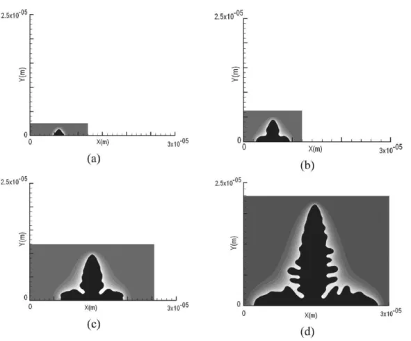
Figures 10a-d shows the dendrite growth during the solidiication process for binary alloy for different times and domain sizes.
In Figure 10a, a dendrite without secondary arms grows from center of the small computational domain with 85 points; solidiication time is 1.33×10⁻⁵ sec. In Figure 10b, the numerical grid with 205 points is larger than that of Figure 10a, due to the dendrite advancing into supercooled liquid. In Figure 10b, one observes only primary arms, with no side branching, the solidiication time is 7.01×10⁻⁵ sec. In Figure 10c, the time for solidiication is 2.06×10⁻⁴ sec insuficient for we observe secondary arms well developed. Finally, in Figure 10d, the time for solidiication is 1.50×10⁻³sec and the numerical grid is 605 points. Here, it is possible to
observe few developed secondary arms away from the dendrite tip during the solidiication process. The asymmetry in the side branches is evinced in Figures 10d. In all of Figure 10, computational convergence is optimized through adoption of a small computational domain around the dendrite.
Figure 11 shows variation of computer run time (in seconds) as a function of primary dendrite length (in
Figure 7. Growth velocity versus radius of dendrite tip.
Figure 8. Comparison of carbon concentration as evaluated:
via the phase-ield model; with Scheil’s equation; and with the Clyne-Kurz equation.
Figure 9. Carbon concentration by region: solid (ϕ= +1), liquid
units of domain size) for binary alloy (Fe-C). The run time required to reach a given length for primary dendrite is about tenth of that with the computational domain of ixed size. The eficiency is guaranteed via adaptive computational domain for phase ield and concentration calculation due to the small computational domain at the beginning of the calculations.
5. Conclusions
In spite of the proven ability of phase-ield models for computation of the pattern evolution in solidiication, they suffer from low computational eficiency. In the computation of a dendrite with side branches, the computational space should be discretized into a mesh with about two million cells. Such a high number leads to a considerable increase of the run time. In the present study, a phase-ield model is introduced with an adaptive computational domain for eficient computational simulation of the dendritic growth in a system for both pure material (Ni) and binary alloy (Fe-C). The method, which is based on the difference in thermal diffusivity for pure material and solute diffusivity in binary alloy, enables us to reduce by about an order of magnitude the run time for simulation of the solidiication via the phase-ield model.
The phase and thermal ields were calculated adaptively only in the regions that satisfy the condition T(I,J) > T0 + 1.1,
for simulation of solidiication in pure material. The phase and concentration ields were calculated in the regions that satisfy the condition C(I, J) > C0 + 1×10
–3, for solidiication
of binary alloy. The computation showed that the dendrite with developed secondary and tertiary arms can be obtained on a personal computer with a much reduced run time. The calculated dendritic morphology displayed a microstructure quite similar to results found in literature and experiments.
Figure 10. Development of the adaptive computational domain for dendritic growth for binary alloy (Fe-C). The numerical grids and
solidiication times are: (a) 85 points, 1.33×10⁻⁵ sec; (b) 205 points, 7.01×10⁻⁵ sec; (c) 400 points, 2.06×10⁻⁴ sec; and (d) 605 points,
1.50×10 − 3 sec.
References
1. Ferreira AF, Silva AJ and Castro JA. Simulation of the solidification
of pure nickel via the phase-field method. Materials Research. 2006; 9(4):349-356.
2. Ode M, Kim SG, Kim WT and Suzuki T. Numerical prediction of the secondary dendrite arm spacing using a phase-field
model. ISIJ International. 2001; 41(4):345-349. http://dx.doi. org/10.2355/isijinternational.41.345.
3. Ferreira AF and Ferreira LO. Microsegregation in Fe-C-P ternary alloys using a phase-field model. Journal of the Brazilian Society of Mechanical Sciences and Engineering. 2009; 31(3):173-180.
http://dx.doi.org/10.1590/S1678-58782009000300002.
4. Salvino IM, Ferreira LO and Ferreira AF. Simulation of microsegregation in multicomponent alloys during solidification. Steel Research International. 2012; 83(8):723-732. http://dx.doi. org/10.1002/srin.201200003.
5. Xu Y, McDonough JM and Tagavi KA. A numerical procedure
for solving 2D phase-field model. Journal of Computational
Physics. 2006; 218(2):770-793. http://dx.doi.org/10.1016/j. jcp.2006.03.007.
6. Moelans N, Blanpain B and Wollants P. An introduction to
phase-field modeling of microstructure evolution. Computer
Coupling of Phase Diagrams and Thermochemistry. 2008; 32(2):268-294. http://dx.doi.org/10.1016/j.calphad.2007.11.003.
7. Boettinger WJ, Warren JA, Beckermann C and Karma A.
Phase-field simulation of solidification. Annual Review of Materials Research. 2002; 32(1):163-194. http://dx.doi.org/10.1146/ annurev.matsci.32.101901.155803.
8. Kim SG, Kim WT, Lee JS, Ode M and Suzuki T. Large scale simulation of dendritic growth in pure undercooled melt by
phase-field model. ISIJ International. 1999; 39(4):335-340. http://dx.doi.org/10.2355/isijinternational.39.335.
9. Stefanescu DM. Science and engineering of casting solidiication.
2nd ed. Ohio: Springer; 2009. p. 160.
10. Altundas YB and Caginalp G. Computations of dendrites in 3-D and comparison with microgravity experiments. Journal
of Statistical Physics. 2003; 110(3-6):1055-1067. http://dx.doi. org/10.1023/A:1022140725763.
11. Campos MP Fo. and Davies GJ. Solidiicação e fundição de metais e suas liga.Rio de Janeiro: Livros Técnicos e Científicos;