Alexandre Furtado Ferreira
[email protected] Universidade Federal Fluminense Graduate Program in Metallurgical EngineeringAvenida dos Trabalhadores, 420 27255-125 Volta Redonda, RJ, Brazil
Leonardo de Olivé Ferreira
[email protected] Universidade Federal Fluminense Mechanical Engineering and Applied MathematicsAvenida dos Trabalhadores, 420 27255-125 Volta Redonda, RJ, Brazil
Abner da Costa Assis
[email protected] Universidade Federal Fluminense Metallurgical Engineering Avenida dos Trabalhadores, 420 27255-125 Volta Redonda, RJ, BrazilNumerical Simulation of the
Solidification of Pure Melt by a
Phase-Field Model Using an Adaptive
Computation Domain
In this paper, we present a phase-field model with a grid based on the Finite-Difference Method, for improvement of computational efficiency and reducing the memory size requirement. The numerical technique, which is based on the temperature change of the pure material, enables us to use, in the initial steps of the computation, a very small computational domain. Subsequently, in the course of the simulation of the solidification process, the computation domain expands around the dendrite. The computation showed that the dendrite with well-developed secondary arms can be obtained with low computation time and moderate memory demand. The computational efficiency of this numerical technique, the microstructural evolution during the solidification, and competitive growth between side-branches are discussed.
Keywords: computer simulation, dendrites, phase field, nickel, numerical efficiency
Introduction1
The understanding and modeling of dendritic growth has remained a central theme of solidification research for many years. Understanding the solidification process is of great importance because the resulting microstructures determine the properties of the material. Although there have been significant developments in understanding dendritic structures in the past decades, our knowledge of the dendritic growth is based on experiments and idealized theoretical models. On the other hand, phase-field models are known to be very powerful in describing non-equilibrium dendritic evolution. They are very efficient because, in the numerical treatment based on them, all the governing equations are written for the whole domain without distinguishing the interface from the solid and liquid phases. Furthermore, direct tracking of the interface position is not needed during numerical simulation of the solidification process. The Phase-field models were developed mainly for studying solidification of pure materials, being then extended to the solidification of binary and ternary alloys.
Recently, Xu et al. (2006) used phase-field models focused on pure materials. Their paper presented a detailed numerical method and algorithm for solving two-dimensional (2-D) phase-field models. Comparison between the fully-coupled and sequential techniques showed that CPU time of the second approach is approximate 10% greater than that of the first one. However, the sequential method is chosen for computations in order to reduce storage requirements as much as possible. The authors found that the numerical results capture well the complex physics of the solidification problem. Consistent with physical reality, the computed critical radius indicates existence of a critical value for a nucleus to grow in the phase field simulation. Moreover, the critical radius decreases linearly with increasing Stefan number, which means that, if the Stefan number is large enough, solidification always takes place, no matter what the initial conditions are. In addition, they studied dendrite shapes at different degrees of supercooling; the results are in agreement with the experimental results.
Moelans et al. (2008) published a paper presenting an introduction to phase-field models and an overview of their possibilities. Amongst those, as listed by the authors, was the simulation of solidification processes, precipitate growth and, more
Paper accepted December, 2010. Technical Editor: Amir Oliveira Junior
recently, an application to solid-state phase transformations like the austenite-to-ferrite transformation in steels, dislocation dynamics, as well as crack nucleation and propagation. Achievements are expanding rapidly, due to improved modeling and implementation techniques and growing computer capacity.
From a somewhat more theoretical standpoint, it should be noted that the interface morphology of the solidification front calculated by phase-field models reproduces the known patterns of a dendrite structure. The state of the domain is represented by the distribution of a single variable known as the order parameter, , or phase-field variable. In this study, the solid state is represented by
, while, in the liquid region, . The region in which changes progressively from to is defined as the solid/liquid interface.
In spite of phase-field models being suitable for simulating solidification processes, as mentioned by Moelans et al. (2008), they suffer from low computational efficiency. For example, for computation of a dendrite with side-branches, the computational domain should be discretized into one million points. Thus, the computational stability condition in an explicit finite scheme can be guaranteed only with a very small time step. Xu et al. (2006) show a sequential method to reduce required storage during the calculations of the solidification process. In this study, on the other hand, we present a numerical technique for the improvement of computational efficiency for computation of dendritic evolution in solidification processes in pure undercooled melts. At the start of the solidification process, there is a solid nucleus placed in the very small computational domain. The goal of this technique is for the computational domain to grow around the dendrite and fix the grid spacing (XYxm, square grid), while solidification advances into the liquid region. The growth around the dendrite is controlled according with the thermal diffusivity of the material in the liquid region.
Nomenclature
Cp = specific heat at constant pressure, J/m 3
K D = thermal diffusivity, m2/sec
g() = function in the phase-field models h() = function in the phase-field models
I = number of node points in the x direction j = anisotropy mode number
J = number of node points in the y direction K = iteration counter
Kmax = maximum number of iterations
M = mobility of the phase-field variable, m3/sec·J Nx = grid numbering in x-direction
Ny = grid numbering in y-direction
r = randomly-generated number between +1 and –1
t = time step, sec
T0 = initial undercooled temperature, K
Tm = melting temperature, K
X = grid spacing in x-direction, m
Y = grid spacing in y-direction, m
w = interface thickness-associated parameter, J/m3 Greek Symbols
= noise amplitude factor
= anisotropy constant, dimensionless
0 = interface thickness, (J/m)1/2 = order parameter, dimensionless
= orientation of the normal to the interface with respect to the x-axis, rad
0 = interface orientation with the maximum anisotropy, rad 0 = interface width, m
= kinetic coefficient, m/sec, K
= material density, kg/m3
0 = interface energy, J/m
2
= order parameter
x = derivative of the order parameter along the x direction
y = derivative of the order parameter along the y direction
Phase Field Modeling
The time-evolution equation of the energy transport can be described as in the work of Kim et al. (1999):
t h C H T D t T p
2 (1)In Eq. (1), D is the thermal diffusivity, H is the latent heat, considered positive for solidification, is the material density, assumed the same for both solid and liquid, Cp is the specific heat.
Equation (1) is linked to the phase-field equation by a source term, t. The evolution of the 2-D phase-field is described in the work of Kim et al. (1999) as:
´ ´( ) ´( ) ( ) ´ ) ( .( 1 2 m m T T T H h wg y x x y t M (2)The term on the left-hand side, t, represents the time variation of the order parameter . On the right-hand side, the first term is a diffusivity term, whereas the second and third terms represent the anisotropy. The product wg´ determines the distribution of the excess free-energy at the interface. The last product on the right-hand side translates the driving force behind the solidification process. While g´ represents the free energy in the solidification process, h´ is the derivative of the so-called “smoothing” function. Here, M is the mobility of the phase-field variable, and w are parameters associated with the interfacial energy and interface
thickness, respectively, and Tm is the melting temperature. The
function h varies monotonically from h to h and h´h´. In this study, we chose a widely used means to define h and g in phase-field models, as expressed in the works of Furtado et al. (2006) and Lee and Suzuki (1999):
2
3 6 15 10 ) (
h (3)
2 21
)
(
g
(4)To take anisotropy into account, is defined as in Furtado et al. (2006):
0
0 1 cos
)
(
M j (5)
The parameter represents the degree of anisotropy and j is a mode number of anisotropy. gives the orientation of the normal to the interface with respect to the x-axis, so that 0 is the interface orientation when the anisotropy is maximal. From the work of Kim et al. (1999), it is easy to conclude that
x y
) (
tan (6)
The three parameters in the phase-field equation, M, 0 and w, are related to the interface kinetic coefficient (), interface energy (), and interface width (). They are expressed in the work of Furtado et al. (2006) as
0 0 6 . 6
w (7)
0 0 0 2.73
(8)
0 73 . 2 H T M m
(9)
In the present study, we introduce a 2-D phase-field model with anisotropy and apply it to the solidification of a supercooled melt of pure nickel. This phase-field model is based on the simultaneous solution of the energy and phase-field equations. Phase-field modeling assumes the growth of a nucleus in the liquid phase. The boundary condition for the order parameter is a zero-flux condition, while an adiabatic process was assumed for the heat flux. Numerical values for the model parameters and physical properties are presented in the results section.
Numerical Method
Equations (1) and (2) were solved by an explicit finite-difference method, with a mesh sufficiently refined to describe details of the dendrites. Considering the pure-metal case, convergence is possible for values of tX. However, in order to observe the growth of thermal dendrites, the calculation must be done according to the time scale of the thermal diffusion. For this reason, it was necessary to use tX4D.
The anti-symmetrical side branching from primary arms around the dendrite tip is known to be possible only with the existence of a noise source in the phase-field equation. Therefore, random noise was added to Eq. (2), in the same way as described in the work of Warren and Boettinger (1995):
2 2(1 )
16
r
where r is a randomly-generated number between and and is a noise amplitude factor. From Eq. (10), the noise can be seen to reach its maximum value for , being null at = 0 and = +1. Performing the computations with a numerical grid of 200 x 200 points with parameters determined in the previous section and the physical properties of nickel, it was not feasible to obtain a dendrite with developed secondary arms, due to the small computation domain. Dendrites with fully developed side branches necessitate a computational domain with several million points. However, computation with such a large computational domain is restricted not only by the computational efficiency, but also by memory size. In the present study, we develop a simple numerical technique in order to improve efficiency. Both phase-field models presented in this article, one with an adaptive computation domain and one with a computation domain of fixed size, were constructed with the same grid spacing (XY m). The difference is in the number of nodes of the computational domain. In the first model, the computational domain is very small in the initial steps of the computation; consequently, the computational efficiency is improved and the memory size requirement is reduced. In the second model, in the initial steps of the computation the computational domain is very large, thereby reducing computational efficiency and the memory size requirement is increased.
The phase and energy transport equations were solved in a computational domain divided into square grids of I×J, with a grid spacing of XY not only for the thermal field, but also for calculation of the phase field. The thermal field TI,J and phase field
I,J at each point in the grid I,J are known from the previous step. For each point I,J in the grid, a real value I,J, which describes the phase state of the grid, is assigned I,J to indicate the grid in the liquid state and I,J for the solid state. The ensemble of all grid points with I,J is taken to represent the interfacial region. At each time step, only the interface-region value of the phase field I,J is calculated from previous values, by the explicit finite-difference form of Eq. (2).
The transient response of the phase-field equation is controlled by the product M. This parameter acts in the phase-field model similarly to the thermal diffusivity D in the energy transport equation. As the work of Furtado (2005) pointed out, in the formation of a dendritic morphology it is important that thermal diffusivity becomes greater than its similar term, M. A greater value of D forces the thermal front to be always ahead of the solidification interface. Hence, there is always a thermal gradient ahead of the solidification front. In this study, the thermal boundary layer is defined as a region with TI,JT0, where T0 is a given initial undercooled temperature.
In the phase-field models, the computational domain used for this kind of simulation should be discretized into about one million grid points. In this study, in the initial stage of solidification the computational domain used to calculate dendrite evolution is rather small, about 200 x 200 points. If the condition TI,JT0 at
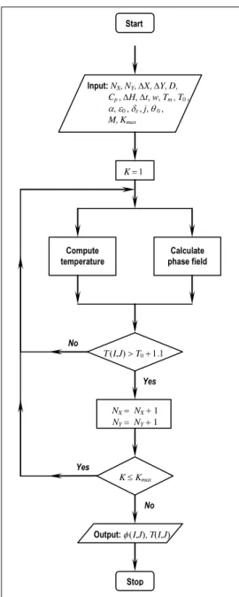
I,J in the square region is satisfied, the adaptive computational domain grows around the dendrite. Whenever the condition is satisfied, new temperature TI,J and phase I,J at the current time step are calculated from the explicit finite-difference method from the values in previous steps. If the condition just stated is not satisfied, the computational domain does not grow. The new temperature TI,J and phase I,J are then calculated from the values in previous steps for a small-size domain. In the present paper, we developed a numerical technique with moderate memory and enhanced computational efficiency, especially at the initial stage of solidification. The calculations were performed on an Intel 2 Quad processor, with 1.38GB RAM. The block diagram in Fig. 1 shows the flow of information in the numerical program.
Figure 1. The phase-field model for pure-metal solidification with adaptive computational domain.
Results and Discussion
Phase-field simulation of dendritic solidification
The parameters and properties adopted in this study are summarized in Tables 1 and 2, respectively.
Table 1. Model parameters (Ni).
Anisotropy constant, 0.025 Interface thickness, o 2.01 10 4 (J/m)1/2 Free energy factor, w 0.61 10 8 J/m3 Interface mobility, M 13.47m3/secJ Grid spacing (X) 2 10 8 m Grid spacing (Y) 2 10 8 m Time step, t 1 10 12 sec Noise amplitude factor, 0.025
Start
Input: NX, NY, X, Y, D,
____ Cp , H, t, w, Tm , T0,
____, 0, , j, 0,
____ M, Kmax
K
Compute temperature
Calculate phase field
TI,JT0
NX NX1
NY NY1
KKmax
Output:I,J, TI,J
Stop
Yes
Yes
Table 2. Material properties of Ni (Kim et al., 1999).
Interface energy, o 0.37J/m
2
Kinetic coefficient at interface, 2m/s K Melting temperature (Tm) 1728 K
Latent heat (H) 2.35 10 9J/m3 Thermal diffusivity (D) 1.55 10− 5m2/s Specific heat (Cp) 5.42 10 6J/m3 K
Interface width (2 o) 8 10− 8m
Dendritic growth analysis is popular in phase field studies and there are lots of application examples for pure materials like those featured in Kobayashi (1993) and Andersson (2002), as well as phase-field models for solidification of binary alloys as, e.g., the works of McFadden et al. (1993) and Wheeler et al. (1993), and ternary alloys, like in the paper by Lee and Suzuki (1999).
The first numerical simulation in this study, using a phase-field model, was conducted for the study of free dendrite growth in a pure material. Figure 2 shows a calculated dendrite, growing from a seed at the central region of the computational domain.
Figure 2. Dendrite calculated with a 1400 x 1400 point grid, where the dendrite started to grow from a seed at the central region. Solidification time was 3.79 x10− 7 sec.
Figure 2 depicts the simulation of a nickel dendrite calculated with a numerical grid of 1400 x 1400 points. In this simulation, a dendrite is presented with secondary and tertiary arms. The secondary arm increases with the distance behind the primary dendrite tip. The asymmetry in the side branch of the primary arms observed in Fig. 2 is due to a noise source added to the phase-field equation. The tertiary arms occur only at one side of the secondary arms. This asymmetry seems to be related to the thermal field distribution. The preferential direction of tertiary arm growth coincides with that of release of latent heat. This was observed in experiments on dendritic growth in undercooled melts. In all simulations carried out for the present study, the value of the anisotropy mode number is J. Also, we choose in Eq. (5). Therefore, the interface orientation with respect to the maximum anisotropy is at the diagonal direction of a grid, entailing preferential dendritic growth along this direction. An adiabatic process was assumed for the heat flux. The boundary condition for is a zero-flux condition. We zoom in on the dendrite tip (Fig. 2) to show the results for the phase field. This is presented in Fig. 3.
Figure 3. Extended region from tip of dendrite.
Figure 3 shows the results for order parameter () calculated in the interface region. As previously mentioned, the interface is determined implicitly in phase-field models by values of calculated between 0 and 1. A grid spacing of XY m is assumed constant everywhere in the domain, including the interface region.
To exhibit the similarities between the dendrites calculated in the present paper and those described in the literature, we introduce Fig. 4. In that figure, both pictures display: a) the secondary arms; b) the secondary arm increase with distance behind the primary dendrite tip; c) the asymmetry of the side branch found in the secondary arms; and d) the secondary arms growth rigorously perpendicular to the primary arm.
Figure 4. (a) Present calculation and (b) dendrite found in the literature (Prates, 1978).
Phase-field simulation and computational efficiency
In order to test the computational efficiency of our numerical technique, we compared the computer run time for the calculation of dendritic growth in undercooled melts using a phase-field model with and without an adaptive computational domain.
(a) (b)
(c) (d)
Figure 5. Development of the adaptive computational domain for dendritic growth. The numerical grids and solidification times are: (a) 85 x 85 points, 4.47 x 10− 9 sec; (b) 205 x 205 points, 3.62 x 10− 8 sec; (c) 405 x 405 points, 9.35 x 10− 8 sec; and (d) 605 x 605 points, 1.50 x 10− 7 sec.
Figures 5(a)-(d) show the development of the adaptive computational domain for dendritic growth. In Fig. 5(a), the dendrite started to grow from a nucleus added at the center of the computational domain with 85x85 points, solidification time being equal to 4.47x10⁻⁹ sec, insufficient for growth of primary and secondary arms. In Fig. 5(b), the numerical grid (205x205) is larger than that of Fig. 5(a) (85x85), due to the dendrite tip advancing into supercooled liquid during the solidification process. In Fig. 5(b), one observes only primary arms, with no side branching, for a solidification time of 3.62x10⁻⁸ sec. In Fig. 5(c), the time for solidification (9.35x10⁻⁸ sec) is sufficient for the growth of secondary arms. Finally, in Fig. 5(d), the time for solidification is 1.50x10⁻⁷ sec and the numerical grid comprises 605x605 points. Here, it is possible to observe well-developed secondary arms away from the dendrite tip, while small side branches compete with each other shortly behind the dendrite tip. The asymmetry in the side branches is evinced in Figs. 5(c) and (d). This follows from the thermal field distribution. Again, side branching prefers the direction of latent heat release. In all of Fig. 5, computational convergence is optimized through adoption of a small computational domain around the dendrite.
Figure 6 shows variation of computer run time (in seconds) as a function of primary dendrite length (in units of domain size). There, the open and solid circles are for the adaptive computational domain and a computational domain of fixed size, respectively. One can see that, with the adaptive computational domain, the run time required to reach a given primary dendrite growth is about a tenth of that with the computational domain of fixed size. Computational efficiency is guaranteed by using an adaptive computational domain for phase field and thermal calculation. Because the computational domain is small at the beginning of the calculations, convergence is optimized. Using the phase-field model with an adaptive computational domain for simulation of the solidification process, the calculation of dendritic growth is carried through with a computational domain sufficiently small for the phase field and thermal calculations. Increasing the primary dendrite length, one finds that the run-time versus primary-dendrite-length plot will tend to exhibit an exponential-like behavior.
Figure 6. Variation of computer run time as a function of primary dendrite length, in units of points.
Figures 7(a) and 7(b) show the dendritic patterns obtained by our phase-field model with an adaptive computational domain and a computational domain of fixed size, respectively. A nucleus was placed at the central point of the domain. The initial and boundary conditions used in this simulation with an adaptive computation domain are identical to those adopted in the simulation with a computation domain of fixed size. In both Figs. 7(a) and 7(b), the initial undercooled temperature is 1468 K. If different degrees of supercooling are adopted for the simulations, dendritic formation with different morphologies will ensue. The average length of the primary dendrites in Fig. 7(a) is 1.02x10⁻⁵ m, and 9.9x10⁻⁶ m in Fig. 7(b). The run times for Figs. 7(a) and 7(b) are 1.2x10⁴ sec and 1.0x10⁵ sec, respectively. The growth velocity of the dendrite tip in Fig. 7(a) is about 49.13 m/sec, whereas it is roughly 46.1 m/sec in Fig. 7(b).
(a) (b)
Figure 7. Dendritic patterns obtained by (a) the Phase Field Model with an adaptive computational domain and (b) the Phase Field Model with a computational domain of fixed size.
computational domain of fixed size. As for improvements in computational efficiency, however, the slight differences in morphology cannot be considered as an obstacle for the phase-field model with an adaptive computational domain. This method can be very useful for solidification simulation via phase-field model.
Conclusions
In spite of the proven ability of phase-field models for computation of the pattern evolution in solidification, they suffer from low computational efficiency. In the computation of a dendrite with side branches, the computational space should be discretized into a mesh with about two million cells. Such a high number leads to a considerable increase of the run time.
In the present study, a phase-field model is introduced with an adaptive computational domain for efficient computational simulation of the dendritic growth in a system of pure undercooled melts. The method, which is based on the difference in thermal diffusivity in pure materials, enables us to reduce by about an order of magnitude the run time for simulation of the solidification via Phase Field Model.
The phase and thermal fields were calculated adaptively only in the regions that satisfy the condition TI,JT0. The computation showed that the dendrite with well-developed secondary and tertiary arms can be obtained on a personal computer with a much reduced run time. The calculated dendritic morphology displayed a microstructure quite similar to results found in literature and experiments.
References
Andersson, C., 2002, “Phase-Field Simulation of Dendritic
Solidification”, Doctoral dissertation, Royal Institute of Technology,
Stockholm, Sweden.
Furtado, A.F., 2005, “Modelamento do Processo de Solidificação e Formação de Microestrutura pelo Método do Campo de Fase” (Phase-Field Modeling of the Solidification and Microstructure Formation Process; in Portuguese), Ph.D. Thesis, Universidade Federal Fluminense, Volta Redonda, RJ, Brazil.
Furtado, A.F., Castro, J.A., and Silva, A.J., 2006, “Simulation of the Solidification of Pure Nickel via the Phase-Field Method”, Materials Research, Vol. 9, No. 4, pp. 349-356.
Kim, S.G., Kim, W.T., Lee, J.S., Ode, M., and Suzuki, T., 1999, “Large
Scale Simulation of Dendritic Growth in Pure Undercooled Melt by Phase-Field Model”, ISIJ International, Vol. 39, No. 4, pp. 335-340.
Kobayashi, R., 1993, “Modeling and Numerical Simulations of Dendritic Crystal Growth”, Physical Review D, Vol. 63, pp. 410-423.
Lee, J.S., and Suzuki, T., 1999, “Numerical Simulation of Isothermal Dendritic Growth by Phase-Field Model”, ISIJ International, Vol. 39, No. 3, pp. 246-252.
McFadden, G.B., Wheeler, A.A., Braun, R.J., Coeriell, S.R., 1993, “Phase
-Field Models for Anisotropic Interfaces”, Physical Review E, Vol. 48, pp. 2016-2024.
Moelans, N., Blanpain, B., Wollants, P., 2008, “An Introduction to
Phase-Field Modeling of Microstructure Evolution”, Computer Coupling of Phase Diagrams and Thermochemistry, Vol. 32, p. 268-294.
Prates, M.C.F., Davies, G.J., 1978, “Solidificação e Fundição de Metais
e Suas Ligas” (Solidification and Casting of Metals and their Alloys; in
Portuguese), Livros Técnicos e Científicos, Rio de Janeiro, RJ, Brazil, 59 p.
Warren, J.A., and Boettinger, W.J., 1995, “Prediction of Dendritic Growth and Microsegregation Patterns in a Binary Alloy Using the
Phase-Field Model”, Acta Metall. Mater., Vol. 43, No. 2, pp. 689-703.
Wheeler, A.A., Murray, B.T., and Schaefer, R.J., 1993, “Computational
of Dendrites Using a Phase-Field Model”, Physical Review D, Vol. 66, pp. 243-262.
Xu, Y., McDonough, J.M., and Tagavi, K.A., 2006, “A Numerical