Matéria (Rio J.) vol.19 número4

ISSN 1517-7076 artigo 11569, pp.389-394, 2014

Molecular dynamic study of the jet noise

about the micro-scale tube

Yong-Fei XUE 1, 2, Jun-Long XIE 1

Huan-Lin DUAN 2, Ke-Qi WU 1

1

School of Energy and Power Engineering, Huazhong university of science and technology, Wuhan 430074, China e-mail: [email protected]; [email protected]; [email protected]

2

College of Civil Engineering, Henan institute of engineering, Zhengzhou 450007, Henan, China e-mail: [email protected]; [email protected].

ABSTRACT

This paper studies the two-dimensional micro-scale molecular simulations of the jet flow using Lagrange discrete systems and adopting Andresen flexible constraint mechanism. At the effects of different excitation conditions and boundary conditions, the low Mach number flow field and sound field are obtained, and characteristic results are given. At the jet flow and pipe flow regions, particles velocities distribution is consistent with traditional method. There are many small groups which have a bigger velocity value, and form the disturbance sources. The stronger interaction with the tube wall produces greater sound pressure, thus random collisions method at the tube wall is effective to deal with sound propagation problem. Therefore, this paper offers preliminary and calculated basis for the molecular and macroscopic quantum aerodynamic problems.

Key words: jet flow, sound propagation, constraint molecular dynamics, Lagrange density, micro scale tube

1. INTRODUCTION

The traditional top-down fluid numerical simulations often focus on the discrete truncation errors, but ignore the physical conservation and numerical stability. Then the microscopic discrete model can be discovered the nature of the macro phenomena profoundly, because it is bottom-up approach for understanding the

macro-micro particles and fluid phenomena essentials [1]. Lattice Boltzmann method has been the most

successful applications [2]. From lattice Boltzmann method to molecular level study, the main considering

objects changes into very small scale, so it would be more able to reveal acoustic mechanism.

Once the atomic natures of matters are determined, quantum mechanics describes the microscopic world, the molecular composition and the microscopic behavior state of particles. Thus makes the situation

become more complicated. So the molecular dynamics simulation study is widely used [3, 4]. On the other

hand, due to the traditional jet flow sound caused by the traditional flow has been affected a lot of attention

[5], and these results usually adopt nanometer size, need the huge amount of computation, so the research

literatures are rarely reported about jet at molecular dynamics levels. This paper would introduce the high-performance computing method, and study the low Reynolds-number jet flow fields by molecular dynamics method, to provide a sound basis for the correct understanding of the micro-scale sound spread phenomenon, to explore microscopic mechanism of the jet sound.

2. SIMULATION MODELS AND PRINCIPLES

The air is a mixture with oxygen and nitrogen molecules by a certain mass ratio. According to the literature

values [6, 7], the energy and length parameters use the Lorentz-Berthelot mixing rule [8]. Its potential energy

function models are the two-body Lennard-Jones potential model [3]. The physical simulations are

*

r r  (1)

* ₍ 2 2 0.5₎

t  t  m (2)

* B

T k T  (3)

* 3

m

  (4)

Where r* is dimensional length, r is diameter [nm],  is length parameter [nm], t* is dimensional

time; t is time[s], m is mass [kg],



[K], kB is Boltzmann constant, ρ* is dimensional density, and ρis density [kg/m3].

Analog pipeline size is 250 angstroms wide, and 1200 angstroms length. The particles at sidewall are

arranged as looped and compact particle forms, named case 1 and case 2. Outer flow field size is 3000×8000

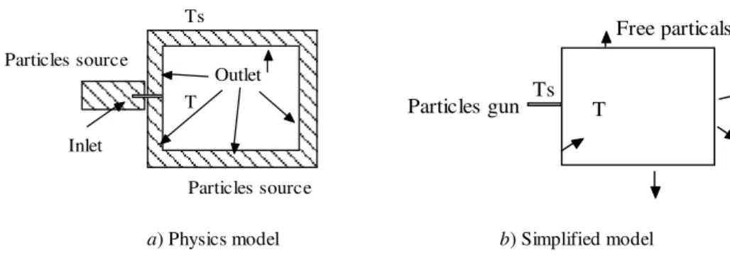
(1200×3200) square angstroms. Calculation model is shown in fig. 1, the tube wall is a solid boundary on

the pipe length, and the other boundary is the gas boundary. Import is simplified as a particle gun, producing various velocities continuously. At the outlet boundary, flow is freely.

T Ts

Particles source

Particles source Inlet

Outlet

T Ts Particles gun

Free particals

a) Physics model b) Simplified model

Figure 1: Calculation model

According to the ideal gas characteristic, the system macro-pressure is as below [3]:

ij ij B

3PV r ( )r 3Nk T

 





P



(

Nk T





r f

/ 3) /

V

Where P is pressure [Pa], V is volume [m3], N is number of molecules, rij is distance[nm] between

molecule i and j, and fij is Lennard-Jones force [N].

Based from the relationship between the internal energy and temperature, kinetic energy is:





i

2

kinetic i / 2 0.5 B 3 - c

E 



Where Ekinetic is kinetic energy [J], p is momentum [kg·m/s], and Nc is the number of molecules at

equilibrium statement. So, the temperature is directly controlled by the internal energy. More, we can add flexible control on the total system temperature, and temperature control factor as below:

0.5 0

{1 [ (t T T t( ))] / [ T t( )]}

Where λ is temperature control factor, δ is space step length [nm], τ is relaxation factor, and T0 is

equilibrium temperature [K].

Weakened the long-range potential to bring direct truncated non-physical factors, the potential force

are softened by math technology [3]. At the inlet, the velocities of particles are displayed approximate

logarithmic distribution [5]. Definition of grid position is as (x, y), the position of equilibrium by the

disturbance and displacement is as η (ηi, i = 1, 2.), the discrete macro-pneumatic system using Lagrange

density of the sound field representation [9]:

2 2

0 0 0

[

2

(

) ] / 2

LD



LT



LV



 

&



p

 

 

p





Where LD is Lagrange density [kg/m3], LT is kinetic density [kg/m3], LV is potential density [kg/m3],

the subscript tag 0 is equilibrium statement,is divergence sign, and ηis displacement [nm].

The initial velocity distribution is according to Maxwell random values, and its’ initial acceleration are

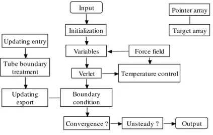
set to zero. At the different time step, the speed values at the import and outlet boundary are reassigned, but the overall region adopts the direct control method in the case 1, and Andresen temperature control in the case 2. The calculated program uses dynamic target arrays to update the number of particles, and pass them

pointer arrays to update its coordinate’s values and the others (as in fig. 2). If the particles is beyond the

control region, then force them freezing, that is stationary. Time step length is taken as 0.0072, and the total

number of time steps is 10+5. The front steps are for fully developed flow, when the flow lines show cyclical

changes, and meet requirements of the state statistical system. The subsequent steps are for the relevant

parameters statistics, such as the sound pressure level (SPL [dB]).

Initialization

Variables

Verlet

Boundary condition

Convergence ?

Force field

Unsteady ?

Pointer array

Target array

Temperature control Updating entry

Tube boundary treatment

Updating export

Output Input

Figure 2: Program chart

Considering the physical mechanisms, system pressures are directly related to the definition style, we consider the following four options about Lagrange density: the direct calculation of sound pressure is arranged as option 1, which is depended on macro parameter (density and pressure). Local parameters are arranged as option 2, mixed parameters are arranged as option 3, and the traditional definition is option 4.

3. FURTHER ANALYSIS AND DISCUSSION

Numerical experiments are carried out firstly in the tube pipeline. With a random velocity along the vertical

direction of the pipe diameter, the results are compared to conventional macro theoryconsistently. Although

the Reynolds number is small, but the molecular layer flow speed still exist a big difference, showing the

nature of turbulence. The existence of the Y velocity shows random features. The viscosity values [m2/s] are

Near-field velocity pulse is relative to the mainstream pulse. The X acceleration value is fluctuating around zero. At central tube, the axial velocity fluctuation is significantly. The Y acceleration value displays small fluctuations, a few larger speed particles clusters still exist. Far-field acceleration value is almost zero.

The Y velocity distribution at 10d place from nozzles is normal (compared with the traditional distribution),

but still with small fluctuations (as in fig. 4). Higher speed flow particle clusters exist, and forms the disturbance source. At the both sides of axis, the velocity distribution changes largely by a few big-speed particles, the overall is symmetry. The negative velocities display back flow and entrainment.

Figure 3: Molecular viscosity at diferent direction

Higher speed flow field particle clusters exist, and forms the disturbance source. Near-field velocity pulse jet boundary relative to the mainstream pulse of small, the X acceleration value is fluctuating around zero; main part is zero (fig. 4). At central pipe, the axial velocity fluctuation significantly, the Y acceleration value displays small fluctuations; X acceleration value is a few larger Speed particles clusters still exist.

Far-field acceleration value is almost zero. The Y velocity distribution at 10 d place from nozzles is normal

(compared with the distribution of the traditional number), but still with small fluctuations. At the both sides of axis, the velocity distribution and instability changes largely by few big-speed particles, the overall is symmetry. The negative velocity display back flow and entrainment.

a) Shaft velocity at tube region b) Shaft acceleration at tube region

Figure 4: Flow distributions diagram in tube region in case 1

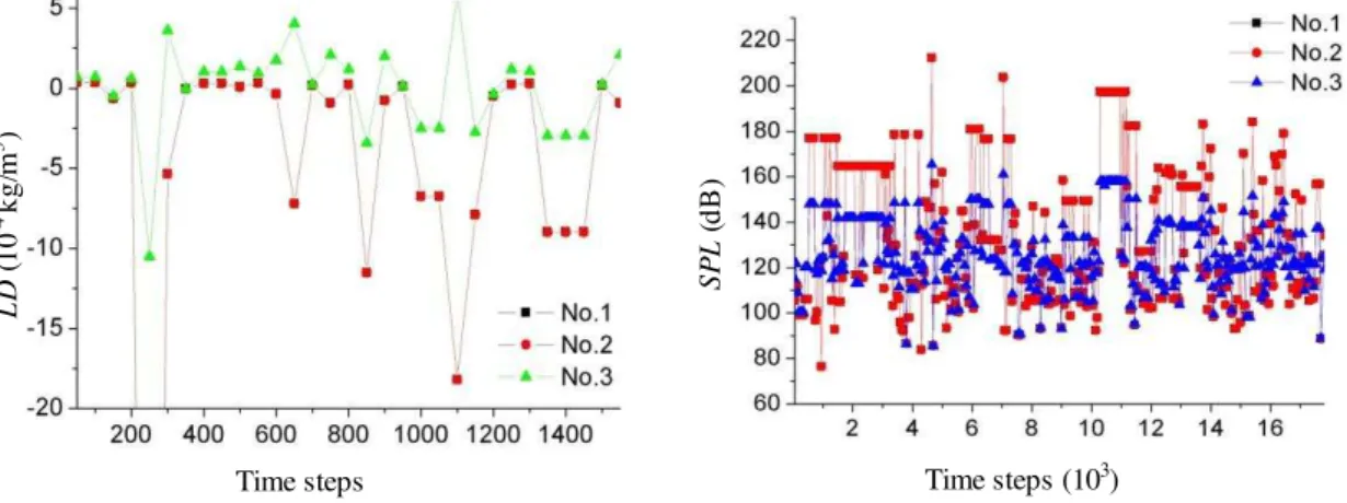
Three programs calculate the Lagrange density can better reflect LD values (as in fig. 5); the fourth

option cannot be calculated. In case 1, The first and third option schemes value calculated is lower than that of the second option, but in case 2 , the first two calculation values are less than that of the third calculation

Y

a

cc

el

e

ra

ti

o

n

(

m

/s

2)

Time step Y/d

V

el

o

ci

ty

(

m

/s

)

T

u

rb

u

le

n

t

v

is

co

si

ty

value.

In case 1, the situation is different from that in the case 2. Considering the wall interactions, three

kinds of SPL are 133, 133 and 126.4dB respectively (fig. 6). At the 10d and 5d distances in case 2, the sound

pressure calculated are 107.6,107.6; 115.5dB 115.6; 115.6, 117dB respectively. The corresponding attenuations are 1.6, 1.6 and 0.3 decibels per pipe diameter.

Figure 5: LD comparison at the 10d place Figure 6: The SPL values at the nozzle

axis in case 1 in case 2

With time step increasing, the density value variation in case 1 shows the two short intervals characteristics firstly, followed by another two large intervals (fig. 7). Further, intervals distance increases, but there exist two basic cycles. This is similar to frequency, and may reflect the inherent characteristics of the jet system.

At the tube monitoring point near the tube wall, the fluid particles collide with the tube wall frequently and randomly. This is the random effects results. The tube wall near the nozzle is the basic source of the jet sound, and it may be the dipole sound source (as in fig. 8).

Figure 7: The density change at the Figure 8: The internal wall speed of a control

5d place of in case 1 in case 2

4. CONCLUSIONS

In this paper, the jet flow field of two-dimensional micro-scale simulation of molecular dynamic, using the Lagrange density mechanism, describes the sound propagation. The main are as bellow:

Compared to the traditional theory, the results compare well with the literature [5]. This shows the

V

el

o

ci

ty

(m

/s

)

Time steps

D

en

si

ty

(k

g

/m

3 )

Time steps(103)

L

D

(1

0

-4 k

g

/m

3 )

Time steps

SP

L

(dB

)

nature of turbulence at all regions, velocity fluctuations displays out random features. The viscosity values are smaller in center region, but bigger at wall aside, no longer a constant.

Lagrange density can be convenient to calculate by the local density and pressure in order to obtain sound pressure, and the traditional definition style cannot get sound pressure values. The sound pressure values are similar to pulse pressure value, and Lagrange densities have two period times characteristics approximately.

At the jet flow field and pipes region, particles velocities distributions are consistent with LBM, but with many small groups which have bigger velocity, and form the disturbance sources.

The strong interaction with the tube wall produces greater sound pressure, such as dipole. Thus random collisions method at the tube wall is effective to deal with sound propagation problem.

Compared with the direct algorithm verlet algorithm is easier to load, effective to control temperature, and of the stalemate to Lagrange conservative force field nature. Molecular Mechanics programming can be

achieved over the use of the space accuracy 10-8 m and the accuracy time 10-12s, which greatly improved the

accuracy of the sound field simulation.

This paper offers preliminary basis and calculated basis for the molecular and macroscopic quantum aerodynamic problems.

5. ACKNOWLEDGEMENT

The authors wish to show our special thanks to the supports by the projects from Natural Science Foundation of China (No. 51376077, No. 50976044), Henan Higher Education Department Project for the excellent youth scholars in China (No. 2011GGJS-176), and Henan Province Education Department Project for the fundamental and advanced research in China (No. 14B470019).

6. BIBLIOGRAPHY

[1] Guo, Z. L., Zheng, C. G., Theory and Applications of Lattice Boltzmann Method, 1 ed., Science Press,

Beijing, China, 2009.

[2] Succi, S., Lattice Boltzmann Equation for Fluid Dynamics and Beyond, 1 ed., Oxford Clarendon Press,

London, England, 2001.

[3] Andrew, R. L., Molecular Modeling Principles and Application, 1 ed., Henry Ling Ltd., Dorchester,

England, 2001.

[4] Frenkel, D., Smit, B., Understanding Molecular Simulation: From Algorithms to Applications, 1 ed.,

Academic Press, San Diego, USA, 2002.

[5] Stromberg, J. L., et al., “Flow Field and Acoustic Properties of Mach Number 0.9 Jet at A Low Reynolds

Number”, J. of Sound and Vib., v. 72, , pp. 159-163, 1980.

[6] Galassi, G., Tildesley, D. J., “Phase Diagrams of Diatomic Molecules: Using the Gibbs Ensemble Monte

Carlo Method”, Molecular Simulations, v. 11, n. 13, pp. 11-24, 1993.

[7] Coon, J. E., Gupta, S., et.el., “Isothermal Isobaric Molecular Dynamics Simulation of Diatomic Liquids

and Their Mixtures”, Chemical Physics, v. 113, n. 1, pp. 43-52, 1987.

[8] Delhommelle, J., Millie, P., “Inadequacy of the Lorentz-Berthelot Combing Rules for Accurate

Predictions of Equilibrium Properties by Molecular Simulation”, Mol. Phys., v. 99, n. 8, pp. 619-625, 2001.