Comparison of machine-learning algorithms to build a
predictive model for detecting undiagnosed diabetes –
ELSA-Brasil: accuracy study
Comparação de algoritmos de aprendizagem de máquina para construir um modelo
preditivo para detecção de diabetes não diagnosticada – ELSA-Brasil: estudo de acurácia
André Rodrigues Olivera
I, Valter Roesler
II, Cirano Iochpe
II, Maria Inês Schmidt
III, Álvaro Vigo
IV, Sandhi Maria Barreto
V,
Bruce Bartholow Duncan
IIIUniversidade Federal do Rio Grande do Sul (UFRGS), Porto Alegre (RS), Brazil
ABSTRACT
CONTEXT AND OBJECTIVE: Type 2 diabetes is a chronic disease associated with a wide range of serious health complications that have a major impact on overall health. The aims here were to develop and valida-te predictive models for devalida-tecting undiagnosed diabevalida-tes using data from the Longitudinal Study of Adult Health (ELSA-Brasil) and to compare the performance of diferent machine-learning algorithms in this task.
DESIGN AND SETTING: Comparison of machine-learning algorithms to develop predictive models using data from ELSA-Brasil.
METHODS: After selecting a subset of 27 candidate variables from the literature, models were built and validated in four sequential steps: (i) parameter tuning with tenfold cross-validation, repeated three times; (ii) automatic variable selection using forward selection, a wrapper strategy with four diferent machine- learning algorithms and tenfold cross-validation (repeated three times), to evaluate each subset of variables; (iii) error estimation of model parameters with tenfold cross-validation, repeated ten times; and (iv) genera-lization testing on an independent dataset. The models were created with the following machine-learning algorithms: logistic regression, artiicial neural network, naïve Bayes, K-nearest neighbor and random forest.
RESULTS: The best models were created using artiicial neural networks and logistic regression. These achieved mean areas under the curve of, respectively, 75.24% and 74.98% in the error estimation step and 74.17% and 74.41% in the generalization testing step.
CONCLUSION: Most of the predictive models produced similar results, and demonstrated the feasibility of identifying individuals with highest probability of having undiagnosed diabetes, through easily-obtained clinical data.
RESUMO
CONTEXTO E OBJETIVO: Diabetes tipo 2 é uma doença crônica associada a graves complicações de saúde, causando grande impacto na saúde global. O objetivo foi desenvolver e validar modelos preditivos para detectar diabetes não diagnosticada utilizando dados do Estudo Longitudinal de Saúde do Adulto (ELSA-Brasil) e comparar o desempenho de diferentes algoritmos de aprendizagem de máquina.
TIPO DE ESTUDO E LOCAL: Comparação de algoritmos de aprendizagem de máquina para o desenvol-vimento de modelos preditivos utilizando dados do ELSA-Brasil.
MÉTODOS: Após selecionar 27 variáveis candidatas a partir da literatura, modelos foram construídos e validados em 4 etapas sequenciais: (i) ainação de parâmetros com validação cruzada (10-fold cross-valida-tion); (ii) seleção automática de variáveis utilizando seleção progressiva, estratégia “wrapper” com quatro algoritmos de aprendizagem de máquina distintos e validação cruzada para avaliar cada subconjunto de variáveis; (iii) estimação de erros dos parâmetros dos modelos com validação cruzada; e (iv) teste de generalização em um conjunto de dados independente. Os modelos foram criados com os seguintes al-goritmos de aprendizagem de máquina: regressão logística, redes neurais artiiciais, naïve Bayes, K vizinhos mais próximos e loresta aleatória.
RESULTADOS: Os melhores modelos foram criados utilizando redes neurais artiiciais e regressão logística alcançando, respectivamente, 75,24% e 74,98% de média de área sob a curva na etapa de estimação de erros e 74,17% e 74,41% na etapa de teste de generalização.
CONCLUSÃO: A maioria dos modelos preditivos produziu resultados semelhantes e demonstrou a via-bilidade de identiicar aqueles com maior probavia-bilidade de ter diabetes não diagnosticada com dados clínicos facilmente obtidos.
IMSc. IT Analyst, Postgraduate Computing Program, Universidade Federal do Rio Grande do Sul (UFRGS), Porto Alegre (RS), Brazil. IIPhD. Professor, Postgraduate Computing Program, Universidade Federal do Rio Grande do Sul (UFRGS), Porto Alegre (RS), Brazil. IIIPhD. Professor, Postgraduate Epidemiology Program and Hospital de Clínicas, Universidade Federal do Rio Grande do Sul (UFRGS), Porto Alegre (RS), Brazil.
IVPhD. Professor, Postgraduate Epidemiology Program, Universidade Federal do Rio Grande do Sul (UFRGS), Porto Alegre (RS), Brazil. VPhD. Professor, Department of Social and Preventive Medicine & Postgraduate Program in Public Health, Universidade Federal de Minas Gerais (UFMG), Belo Horizonte (MG), Brazil.
KEY WORDS:
Supervised machine learning. Decision support techniques. Data mining.
Models, statistical. Diabetes mellitus, type 2.
PALAVRAS-CHAVE:
Aprendizado de máquina supervisionado. Técnicas de apoio para a decisão. Mineração de dados.
INTRODUCTION
Type 2 diabetes is a chronic disease characterized by the body’s inability to eiciently metabolize glucose, which increases blood glucose levels and leads to hyperglycemia. his condition is asso-ciated with a wide range of serious health complications afecting the renal, neurological, cardiac and vascular systems, and it has a major impact on overall health and healthcare costs.1
Recent studies have estimated that around 415 million peo-ple have diabetes, and that the number of cases may increase to 642 million by 2040. In addition, approximately half of these indi-viduals are not aware of their condition, which may further inten-sify the negative consequences of the disease. Diabetes was the main cause of death of nearly ive million people in 2015, and it has been estimated that by 2030 it will become the seventh largest cause of death worldwide.2-4
It is believed that diabetes, like other noncommunicable chronic diseases, is mainly caused by behavioral factors such as poor diet and physical inactivity. Early interventions aimed towards creat-ing lifestyle changes, with or without associated pharmacological therapies, have been proven efective in delaying or preventing type 2 diabetes and its complications. his has led many countries to invest in national programs to prevent this disease. To reduce costs and amplify the results, population-level interventions need to be combined with interventions that are directed towards individuals who are at high risk of developing or already having diabetes,5 so as to focus interventions, at the individual patient level, on those for whom they are most appropriate.
To this end, over recent years, a series of clinical prediction rules have been developed to identify individuals with unknown diabetes or those at high risk of developing diabetes.5-9 However, few of these rules have been drawn up using the most recently developed machine-learning techniques, which potentially have the ability to produce algorithms of greater predictive ability than those developed through the technique most commonly used to date, i.e. multiple logistic regression.
OBJECTIVE
his paper presents the development and comparison of pre-dictive models created from diferent machine-learning tech-niques with the aim of detecting undiagnosed type 2 diabetes, using baseline data from the Longitudinal Study of Adult Health (ELSA-Brasil).
METHODS
hese analyses were performed on data from the baseline survey (2008-2010) of ELSA-Brasil, a multicenter cohort study that had the main aim of investigating multiple factors relating to adult health conditions, including diabetes and cardiovascular dis-eases. he study enrolled 15,105 public servants aged between
35 and 74, at six public higher-education and research institu-tions in diferent regions of Brazil between 2008 and 2010, as has been previously reported in greater detail.10,11 he institutional review boards of the six institutions at which the study was con-ducted gave their approval, and written informed consent was obtained from all participants.
All analyses were performed using R version 3.2.3. he source codes used in the analysis are freely available.
Dataset and preliminary variable selection
Data from the ELSA study baseline were used to create the pre-dictive models. At this baseline, the 15,105 participants were eval-uated through interviews, clinical examinations and laboratory tests. he interviews addressed educational achievement; char-acteristics and composition of home and family; dietary habits; alcohol drinking habits; smoking habits; presence of dyslipidemia or hypertension; physical activity at leisure; sleep quality; medical history; and medication use, among other topics. he examina-tions involved anthropometric measurements and blood and urine tests, among others. he study generated more than 1500 variables for each participant at baseline, as described previously.10,11
A total of 1,473 participants were excluded from the present analyses because they had self-reported diabetes. Another three participants were excluded because some information required for characterizing undiagnosed diabetes was missing. An additional 1,182 participants (8.7%) were excluded from the analyses because data relating to other variables were missing. Among the remain-ing 12,447 participants, 1,359 (11.0%) had undiagnosed diabetes.
Undiagnosed diabetes was considered present when, in the absence of a self-report of diabetes or use of anti-diabetic medica-tion, participants had fasting glucose levels ≥ 126 mg/dl, glucose levels ≥ 200 mg/dl two hours ater a standard 75 g glucose load or had glycated hemoglobin (HbA1c) ≥ 6.5%.
hrough procuring variables in the ELSA dataset that were simi-lar to those investigated in previously published predictive models for detecting diabetes or in situations of high risk of developing diabetes, we selected 27 diabetes risk factors for analysis. Any vari-ables that implied additional costs beyond those of illing out a questionnaire and performing basic anthropometry, such as clinical or laboratory tests, were excluded so that the model obtained could be applied using a straightforward survey and simple anthropo-metric measurements. he inal variable subset was validated by experts, and this resulted in the subset of 27 candidate variables described in Table 1 and Table 2. Table 2 also presents the analy-sis target variable of prevalent diabetes “a_dm”.
Table 1. Numerical variables
Variable identity Minimum Median Mean Maximum SD Variable description
a_cons_est_nacl 0.14 9.67 11.65 3533.00 42.57 Estimated daily salt consumption in grams
a_rcq 0.40 0.89 0.89 1.27 0.09 Waist-hip ratio
a_rendapercapita 27.63 1410.90 1756.34 7884.50 1436.67 Per capita family net income in R$ aia7 0.00 0.00 0.12 7.00 0.68 Bicycle use for transport (days/week)
SD = standard deviation.
Table 2. Categorical variables, including the target variable “a_dm”
Variable identity Number
of levels Frequency in each level Description Possible values
a_ativisica 3 1: 9523; 2: 1735; 3: 1189 Physical activity during
leisure time 1 = weak; 2 = moderate; 3 = strong a_binge 2 0: 10764; 1: 1683 Sporadic excessive
alcohol drinker 0 = no; 1 = yes a_consdiafrutas 2 0: 5434; 1: 7013 Daily consumption of
fruits 0 = no; 1 = yes a_consdiaverduras 2 0: 6003; 1: 6444 Daily consumption of
vegetables 0 = no; 1 = yes a_dm 2 1: 11088; 0: 1359 Diabetes mellitus 0 = yes; 1 = no
a_escolar 4 1: 619; 2: 773; 3: 4219; 4: 6836 Education
1 = middle school not completed or less; 2 = middle school completed; 3 = high school completed; 4 =
university undergraduate course completed a_fumante 3 0: 7212; 1: 3619; 2: 1616 Smoker 0 = never smoked; 1 = former smoker; 2 = smoker a_gidade 4 1: 2899; 2: 5077; 3: 3320; 4: 1151 Age group 1 = 35 to 44 years; 2 = 45 to 54 years; 3 = 55 to 64 years; 4
= 65 to 74 years a_imc2 4 1: 122; 2: 4705; 3: 5011; 4: 2609 Four-level body mass
index
1 = underweight; 2 = eutrophic; 3 = overweight; 4 = obese
a_medanthipert 2 0: 9232; 1: 3215 Use of antihypertensive
drugs 0 = no; 1 = yes a_medoutahip 2 0: 12367; 1: 80 Use of other
antihypertensive drugs 0 = no; 1 = yes a_medredlip 4 0: 11122; 1: 1117; 2: 97; 3: 111 Use of lipid-lowering
drugs
0 = no use; 1 = use of statins; 2 = use of others; 3 = use of more than one class a_sfhfprem 2 0: 12371; 1: 76 Self-reported heart
failure (< 50 years of age) 0 = no; 1 = yes
a_sfmiprem 2 0: 12386; 1: 61
Self-reported myocardial infarction (< 50 years of age)
0 = no; 1 = yes
a_sfrevprem 2 0: 12402; 1: 45
Self-reported revascularization (< 50 years of age)
0 = no; 1 = yes
a_sfstkprem 2 0: 12373; 1: 74 Self-reported stroke
(< 50 years of age 0 = no; 1 = yes a_sintsono 2 0: 8321; 1: 4126 Sleep quality 0 = no; 1 = yes a_sitconj 5 1: 8248; 2: 2028; 3: 1283; 4: 474;
5: 414 Marital status
1 = married; 2 = divorced; 3 = single; 4 = widowed; 5 = other claa2 2 0: 8397; 1: 4050 Pain/discomfort in the
legs while walking (Q2) 0 = no; 1 = yes diea133 3 0: 1038; 1: 11136; 2: 273 Cofee consumption
(Q133) 0 = no; 1 = yes, with cafeine; 2 = yes, decafeinated hfda07 2 0: 3271; 1: 9176 Hypertension, family
history (Q7) 0 = no; 1 = yes hfda11 2 0: 7879; 1: 4568 Diabetes, family history
dataset) was used for generalization tests. he models created were evaluated in terms of area under the receiver operating character-istic curve (AUC), sensitivity, speciicity and balanced accuracy (arithmetic mean of sensitivity and speciicity). he machine-learning algorithm families of logistic regression, artiicial neural network (multilayer perceptron/backpropagation), Bayesian net-work (naïve Bayes classiier), instance-based learning (K-nearest neighbor) and ensemble (random forest) were used.
Machine-learning algorithms
he machine-learning algorithms are briely described below: Logistic regression12 is a well-established classiication tech-nique that is widely used in epidemiological studies. It is gener-ally used as a reference, in comparison with other techniques for analyzing medical data.
Multilayer perceptron/backpropagation13 is the principal artii-cial neural network algorithm. When there is no hidden layer on the network, this algorithm is equivalent to logistic regression, but it can solve more diicult problems with more complex network architectures. he price of using complex architectures is that it produces models that are more diicult to interpret. Additionally, it can be computationally expensive.
Naïve Bayes classiier14 is a type of Bayesian network that, despite enormous simplicity, is able to create models with high predictive power. he algorithm works well with heterogeneous data types and also with missing values, because of the independent treat-ment of each predictor variable for model construction.
K-nearest neighbor (instance-based learning)15 is a classical instance-based learning algorithm in which a new case is classi-ied based on the known class of the nearest neighbor, by means of a majority vote. his type of algorithm is also called lazy learning because there is no model building step and the entire computing procedure (i.e. the search for the nearest neighbor) is performed directly during the prediction. All the cases (training/validation dataset) need to be available during the prediction.
Random forest16 is a machine-learning algorithm from the “ensemble” family of algorithms,17 which creates multiple models (called weak learners) and combines them to make a decision, in order to increase the prediction accuracy. he main idea of this technique is to build a “forest” of random decision “trees” and use them to classify a new case. Each tree is generated using a random variable subset from the candidate’s predictor variables and a ran-dom subset of data, generated by means of bootstrap. his algo-rithm also can be used to estimate variable relevance.
Data preparation
Standardization of numerical variables
Transformation between diferent data types (categorical or numer-ical) was performed by means of binarization or discretization,
when necessary. In binarization, a categorical variable with n levels is transformed into n - 1 dummy variables that have values equal to “1” when the case belongs to the level represented by the dummy variable or “0” otherwise.
In discretization, a numerical variable is transformed into a categorical variable by deining a set of cutof points for that variable, such that the ranges of values between the cutof points correspond to the levels of the categorical variable. he Ameva algorithm18 was used to ind the best cutof points for each numer-ical variable.
General process of model construction and evaluation
he models were built, evaluated and compared using four sequential steps:
1. Parameter tuning;
2. Automatic variable selection; 3. Error estimation; and
4. Generalization testing in an independent dataset.
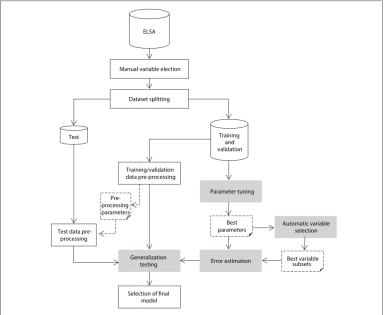
he complete process is depicted in Figure 1. First, manual vari-able preselection was performed as described above (“Manual Variable Selection” box in the Figure). Ater that, 30% of the dataset (“Test” dataset in the Figure), containing 3,709 complete cases, was separated for generalization testing, while the other part (“Training/Validation” dataset in the Figure), containing 8,738 complete cases, was used as the dataset for the irst three steps of the process.
he irst step in model building (“Parameter Tuning” box in
Figure 1) evaluated each machine-learning algorithm with
difer-ent sets of conigurable parameters of the algorithm by means of tenfold cross-validation, repeated three times. In tenfold cross-val-idation, the dataset (training/validation) is divided into ten parts, of which nine are used for training (selecting) a model and the tenth for validation of this model. his process is repeated to cal-culate the validation measurements, such as AUC, while varying the part of the dataset used for validation each time. Finally, the mean of the validation measurements across repeats is calculated. he results from this step (“Best Parameters” item in the Figure), containing the best parameters and cutofs for classiication for each algorithm, were used in the next steps.
The second step (“Automatic Variable Selection” box in
Figure 1) generated four diferent variable subsets using
difer-ent algorithms and cross-validation (using only the best settings found in the preceding step), with the wrapper strategy and a for-ward selection search for automatic variable selection. he best variable subsets found in this step (“Best Variable Subsets” item
in Figure 1) were used in the next steps.
of diferent learning schemes, using the best settings and subsets obtained in the preceding steps.
Finally, the last step (“Generalization Testing” box in Figure 1) evaluated models using only the learning scheme that obtained the best performance for each algorithm in the test dataset that had not previously been used.
he following sections describe each step in more details.
Parameter tuning
his irst step in model building evaluated each algorithm with diferent parameter conigurations to ind out which parameter coniguration produced the best results for each algorithm and data type conversion used. he parameters tested for each algo-rithm are listed in Table 3.
Because of the wide range of possible values for the parameters, a search strategy was adopted. At irst, a limited set of values for
each parameter was selected, and each combination of parameters was evaluated by means of tenfold cross-validation, repeated three times, thus generating 30 models. Each instance of machine learning was tested with and without data discretization. he results from
ELSA
Training and validation Test
Manual variable election
Dataset splitting
Training/validation data pre-processing
Test data pre -processing
Selection of inal model
Parameter tuning
Automatic variable selection
Error estimation Generalization
testing
Pre-processing parameters
Best parameters
Best variable subsets
Figure 1. General process of model construction and evaluation.
Table 3. Parameters analyzed in parameter tuning
Algorithm Parameter Description
Artiicial neural network
Size Number of neurons on hidden layer Decay Weight decay
Skip Direct link between input and output neurons Logistic
regression Epsilon Convergence tolerance value Naïve
Bayes Laplace Real number to control Laplace smoothing K-nearest
neighbor
Minvotes Minimum votes to deine a decision k Number of neighbors considered Random
the 30 models generated in each test were averaged. he param-eter coniguration that produced the best mean AUC was chosen. Moreover, a set of diferent cutofs (predeined by the analyst) to generate the classiication was evaluated to ind out which pro-duced the best classiication on average between the 30 models in terms of balanced accuracy.
Ater that, the results were analyzed and, when necessary, new parameter values and/or cutof points were selected for new tests. In this case, the new values were selected around the values from which the best results had been obtained up to that moment. he idea was to start testing a sparse range of values and then decrease the granularity of the values in order to avoid trying values that were very likely to produce poor results. his search stopped when there was no increase in the predictive power of the models that had been created using the speciic machine-learning algorithm and data type conversion evaluated.
Automatic variable selection
he automatic variable selection step had the aim of inding sub-sets from the 27 candidate variables that could increase the per-formance of the predictive models, compared with other models created using diferent sets of candidate variables.
hese subsets of variables were generated using the wrap-per strategy.19 In this strategy, models are created and evalu-ated by means of a machine-learning algorithm and a validation method, such as cross-validation, using diferent subsets of vari-ables. he subset from which the best performance is achieved, in terms of a criterion such as AUC, is chosen as the best subset. Because of the large number of possible subsets, a heuristic search was used to generate the variable subset candidates that were more likely to create better models, thereby optimizing the process. he main advantage of this method compared with other strate-gies is that it evaluates multiple variables together. he drawback is that, because it depends on a machine-learning algorithm to create/evaluate models, it is possible that the subset of variables that produces the best results using one algorithm can produce bad results when using another algorithm or another parameter setting for the same algorithm.
Four machine-learning algorithms were used: logistic regres-sion, artificial neural network, K-nearest neighbor and naïve Bayes classifier. The random forest algorithm was not included because it already performs an embedded variable selection. The forward selection search strategy was used in modeling because it tends to generate smaller subsets. The same valida-tion technique (tenfold cross-validavalida-tion repeated three times), decision criterion (mean AUC) and dataset partition that had been used in the parameter tuning step were used again in this step. The best parameter settings obtained in the param-eter tuning step were used to configure the paramparam-eters of the
algorithms for this step. Each machine-learning technique gen-erated a distinct subset of variables. The subsets thus gengen-erated were used in the next step.
Error estimation
The error estimation step evaluated each machine-learning algorithm using the parameters obtained in the first step and the subsets generated in the second step, in addition to the original variable subset containing all the candidate variables. This step also served to evaluate the use of discretization. The evaluation was done through tenfold cross-validation, which was repeated ten times to get more reliable prediction perfor-mance estimates.
Generalization testing
Finally, one model was generated from the training/validation dataset for each algorithm, using the best results from the pre-ceding step. hese best models were then evaluated (hold-out evaluation) in the test set, since this generalization testing has the aim of evaluating model behavior when faced with data that was not used in its creation. he results from this evaluation serve as a quality measurement for these models.
Development of an equation for application of the results
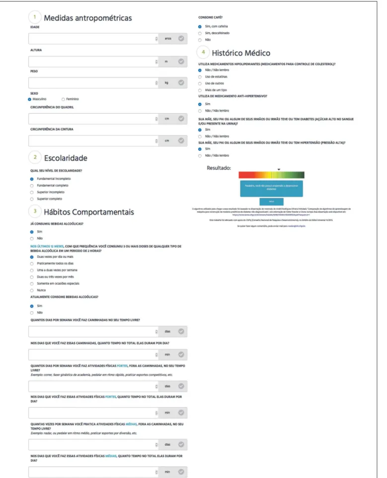
he model with best results from generalization testing was used to create a web tool to apply the questionnaire in practice. he prediction from the logistic regression model for any given individual is calculated by multiplying that individual’s value for each variable in the model by the coeicient derived from the model for that variable, and then summing the results and transforming this sum into a probability of undiagnosed dia-betes using the logistic function. If this probability is above the predetermined cutof (here, 11%), the individual is classiied as positive (at high risk of undiagnosed diabetes); or otherwise, as negative.
RESULTS
Study sample
Parameter tuning
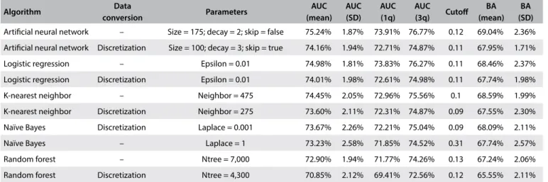
he best parameter coniguration for each data type conversion of each algorithm is depicted in Table 4.
he irst and second columns of Table 4 present the name of the algorithm and whether discretization was used, respectively. he third column shows the values of the parameter coniguration that provided the best result for the machine-learning algorithm and data type conversion of each row. he next four columns pres-ent basic statistics (mean, standard deviation, irst and third quar-tiles and cutof points, respectively) of the AUC obtained in the cross-validation. he eighth column shows the cutof that provided the mean best balanced accuracy (BA) and the last two columns shows the mean balanced accuracy and its standard deviation.
Table 4 shows each machine-learning algorithm with its
dif-ferent data type conversions, sorted in descending order in terms of AUC and balanced accuracy for each algorithm and data type conversion.
Although deining which algorithms produce better results was not the objective of this step, it was possible to gain an initial insight into their predictive powers. In this regard, the best results were produced by artiicial neural networks and logistic regression with mean AUC of 75.24% (row 1) and 74.98% (row 3), respectively.
Table 4 also shows the impact in terms of performance, when
discretization was used in each machine-learning algorithm. For example, performance decreased (around 1% overall and almost 3% in the case of random forest) when the data were discretized in the models generated by all the algorithms except naïve Bayes. In general, the performance behavior of the machine-learning algorithms and conversion remained similar for the next steps.
Another result that can be seen in most cases is the impact on the choice of the parameter settings, caused by the conversion used. For example, the best performance of the artiicial neural network algorithm was achieved without data conversion and with size = 175 (i.e. 175 neurons in the hidden layer). However,
when discretization was used, the best parameter setting changed to size = 100.
he best parameter setting achieved was used to conigure the ive algorithms used for the automatic variable selection step, as well as in further steps.
Results from automatic variable selection
he automatic variable selection step generated four distinct sub-sets of variables as shown in Table 5 (rows 1 to 4): lr-fs, created with logistic regression (fs in the name stands for “forward selection”); ann-fs, created with an artiicial neural network; knn-fs, created with K-nearest neighbor; and nb-fs, created with a naïve Bayes algorithm.
Table 4. Results from parameter tuning
Algorithm Data
conversion Parameters
AUC (mean)
AUC (SD)
AUC (1q)
AUC
(3q) Cutof
BA (mean)
BA (SD)
Artiicial neural network – Size = 175; decay = 2; skip = false 75.24% 1.87% 73.91% 76.77% 0.12 69.04% 2.36% Artiicial neural network Discretization Size = 100; decay = 3; skip = true 74.16% 1.94% 72.71% 74.87% 0.11 67.95% 1.71% Logistic regression – Epsilon = 0.01 74.98% 1.81% 73.83% 76.27% 0.11 68.46% 2.37% Logistic regression Discretization Epsilon = 0.01 74.01% 1.98% 72.61% 74.98% 0.11 67.74% 1.98% K-nearest neighbor – Neighbor = 475 74.45% 2.05% 72.96% 75.56% 0.1 68.59% 1.99% K-nearest neighbor Discretization Neighbor = 275 73.60% 2.11% 72.31% 74.87% 0.09 67.55% 2.30% Naïve Bayes Discretization Laplace = 0.001 73.67% 2.26% 72.21% 75.04% 0.09 68.09% 2.11% Naïve Bayes – Laplace = 1 73.23% 2.58% 71.85% 74.52% 0.31 67.74% 2.57% Random forest – Ntree = 7,000 72.90% 1.94% 71.77% 74.26% 0.13 67.24% 2.06% Random forest Discretization Ntree = 4,300 70.85% 2.12% 69.41% 72.56% 0.12 65.55% 2.11%
AUC = area under the ROC curve; SD = standard deviation; 1q/3q = irst and third quartiles; BA = balanced accuracy.
Table 5. Variable subsets generated in automatic variable selection
Subset Best mean
AUC
Number of
variables Variable names
ann-fs 75.48% 14
a_ativisica, a_binge, a_escolar, a_gidade, a_imc2, a_medanthipert,
a_medredlip, a_rcq, a_rendapercapita, a_ sfhfprem, diea133, hfda07,
hfda11, rcta8.
lr-fs 75.44% 11
a_ativisica, a_binge, a_ escolar, a_gidade, a_imc2,
a_medanthipert, a_rcq, diea133, hfda07, hfda11,
rcta8.
knn-fs 74.94% 12
a_binge, a_escolar, a_gidade, a_imc2, a_medanthipert, a_medoutahip, a_rcq, a_sfmiprem, a_sfstkprem,
hfda07, hfda11, rcta8.
nb-fs 74.47% 10
a_ativisica, a_binge, a_ escolar, a_gidade, a_imc2,
he irst column of Table 5 shows the identiier name of the subset, the second column presents the AUC achieved by the vari-able subset that was chosen for each algorithm, the third shows the number of variables of each subset and the fourth presents these variable names.
he dataset partitions used for this step were the same as used in the parameter tuning step. hus, it is possible to gain an insight into the performance improvement in terms of AUC when using a variable subset instead of using all the variables from the original dataset. Furthermore, merely the fact that a smaller subset was used to create the models is already an advantage because this makes the model and its application much simpler.
Because of the nature of the wrapper strategy, it can be expected that each machine-learning algorithm will present better results when using the variable subset created by the algorithm itself. However, in the next step all the subsets were tested with all the algorithms.
Results from error estimation
he aim of this step was to obtain more reliable error estimates regarding algorithm performance. For this reason, 10 repetitions were used instead of 3, for the repeated tenfold cross-validation, thus generating 100 models instead of 30 for each test.
he machine-learning algorithms were tested using the best parameters found in the irst step (depicted in Table 4), with the variable subsets generated in the second step (described in Table 5), as well as with the original set of variables. Performance was tested with and without discretization.
Table 6 describes the best results obtained for each
machine-learning algorithm, variable subset and data conversion used. Respectively, the columns represent the name of machine-learning algorithm used; data type conversion; variable subset; AUC mean, standard deviation (SD) and irst and third quartiles achieved in cross-validation; and mean and standard deviation of the bal-anced accuracy (BA).
Like in the results from the parameter tuning step, the artii-cial neural network algorithm and logistic regression achieved the best results. Without data conversion, these algorithms produced similar models, with AUC of 75.45% (row 1) and 75.44% (row 4), respectively, each using the variable subset generated with its own algorithm, as expected. K-nearest neighbor and naïve Bayes also reached good results, with AUC of close to 75%. he best results with the naïve Bayes classiier were obtained using a subset of variables other than nb-fs. his was possible because the variable subset search with this algorithm used discretized data following the best results from parameter tuning, while the best result in the current phase was without variable transformation.
Finally, as in the parameter tuning step, random forest pro-duced the worst results. Independent of the subset of variables, this algorithm showed a worse yield in terms of mean AUC.
Table 6 also shows the impact of using a speciic variable
sub-set, compared with the best results obtained from the models generated using the original variable set. his diference is very small: around 0.25% better using the variable subset instead of all the original variables for the artiicial neural network models. he results obtained with a subset of variables were slightly bet-ter (around 0.5%) than the original with logistic regression and K-nearest neighbor models. he best naïve Bayes classiier model result from using a variable subset was more than 1% better than the best result from using all the variables. Finally, random forest models produced the best results using all of the available variables.
Results from generalization testing
In generalization testing, the best learning scheme (which includes data type conversion used, parameter setting, classiica-tion cutof and variable subset) found for each algorithm in the preceding step was evaluated in the test dataset, which had been separated at the beginning of the process and had not been used until this step.
Table 7 shows the best results obtained in the error estimation
phase together with the results obtained in generalization testing. All the algorithms maintained good performance in gener-alization testing. he biggest loss of performance in relation to the error estimate step, as assessed from changes in the AUC, was 1.64% for the K-nearest neighbor algorithm. he artiicial neu-ral network, logistic regression and naïve Bayes had performance losses of 1.30%, 1.03% and 0.80%, respectively. he least loss in generalization testing was 0.458%, achieved by the random for-est algorithm, which produced the worst performance in terms of AUC of all the algorithms. Nevertheless, the worst result was an AUC of 72.35%.
Since the best result from this step in terms of AUC (74.41%) was obtained using logistic regression, and given the easy inter-pretation and applicability of this model, logistic regression was chosen to be used to create the diabetes risk assessment tool.
Web tool proposed for detecting undiagnosed diabetes
Finally, the model generated using the logistic regression algo-rithm in the generalization test was selected to build a web tool for detecting undiagnosed diabetes. his model produced sen-sitivity of 68% and speciicity of 67.2%. he prototype inter-face of the tool is shown in Figure 2. Since the model was con-structed and probably would be used in Brazil, the tool was created in Portuguese.
he inal coeicients of the equation generated are described
in Table 8.
New cases can be classiied using this model, as follows: 1. Standardize the value of the only numerical variable (a_rcq)
Table 6. Error estimation results
Algorithm Transformation Variable subset AUC (mean) AUC (SD) AUC (1q) AUC (3q) BA (mean) BA (SD)
Artiicial neural network - ann-fs 75.45% 1.96% 74.18% 76.96% 69.36% 2.17% Artiicial neural network - lr-fs 75.42% 1.99% 74.07% 77.04% 69.47% 2.14% Artiicial neural network - knn-fs 75.35% 1.98% 74.06% 76.85% 68.90% 2.09% Artiicial neural network - nb-fs 75.33% 2.05% 74.01% 76.95% 69.23% 2.30% Artiicial neural network - original 75.20% 1.96% 73.93% 76.79% 69.00% 2.20% Logistic regression - lr-fs 75.44% 1.98% 74.00% 77.04% 69.30% 2.12% Logistic regression - nb-fs 75.35% 2.02% 73.97% 76.93% 68.93% 2.07% Logistic regression - ann-fs 75.35% 1.96% 74.09% 76.96% 68.91% 2.07% Logistic regression - knn-fs 75.32% 1.95% 74.02% 77.00% 68.76% 2.10% Logistic regression - original 74.94% 1.97% 73.58% 76.53% 68.41% 2.26% K-nearest neighbor - knn-fs 74.98% 2.13% 73.54% 76.83% 68.52% 2.14% K-nearest neighbor - ann-fs 74.80% 2.23% 73.51% 76.59% 68.74% 2.04% K-nearest neighbor - lr-fs 74.77% 2.20% 73.22% 76.69% 68.63% 2.36% K-nearest neighbor - nb-fs 74.68% 2.17% 73.15% 76.43% 68.64% 2.07% K-nearest neighbor - original 74.44% 2.32% 72.99% 76.34% 68.52% 2.14% Naïve Bayes - lr-fs 74.85% 2.20% 73.30% 76.56% 68.95% 2.17% Naïve Bayes - ann-fs 74.71% 2.23% 73.23% 76.43% 68.79% 2.21% Naïve Bayes - knn-fs 74.66% 2.19% 73.20% 76.39% 68.58% 2.14% Naïve Bayes Discretization nb-fs 74.49% 2.12% 72.97% 76.11% 68.15% 2.06% Naïve Bayes Discretization original 73.75% 2.35% 72.16% 75.53% 68.14% 2.15% Random forest - original 72.81% 2.32% 71.61% 74.35% 67.06% 2.34% Random forest - ann-fs 72.10% 2.24% 70.63% 73.79% 64.59% 2.33% Random forest - knn-fs 71.75% 2.40% 70.05% 73.50% 59.72% 2.43% Random forest - lr-fs 70.62% 2.53% 68.92% 72.33% 61.85% 2.56% Random forest - nb-fs 70.42% 2.47% 68.69% 72.24% 61.19% 2.26%
AUC = area under the ROC curve; SD = standard deviation; 1q/3q = irst and third quartiles; BA = balanced accuracy.
Table 7. Generalization testing results compared with those of the error estimation step
Algorithm Error estimation Generalization
AUC BA AUC BA Sensitivity Speciicity
Logistic regression 75.44% 69.30% 74.41% 67.62% 67.99% 67.24% Artiicial neural network 75.45% 69.36% 74.17% 67.78% 66.25% 69.30% Naïve Bayes 74.85% 68.95% 74.06% 68.52% 74.94% 62.1% K-nearest neighbor 74.98% 68.52% 73.34% 67.76% 70.97% 64.55% Random forest 72.81% 67.06% 72.35% 67.50% 67.74% 67.24%
AUC = area under the ROC curve; BA = balanced accuracy.
and dividing the result by the training standard deviation (0.08615528).
2. Binarize the categorical variables;
3. Calculate the sum of the variables created in the preceding steps using the coeicients from Table 8;
4. Add to this sum the value of the intercept term, described in the irst row of Table 8;
5. Calculate the probability of undiagnosed diabetes for a given individual = 1/(1+e-x), where x equals the sum resulting from the preceding steps.
studies include the deinition of the target variable, model objectives and candidate variables, among others. hese models are gener-ally constructed using conventional statistical techniques such as logistic regression and Cox regression. Systematic reviews5,16,24-26 present several such studies: some, like ours, have focused on pre-dicting undiagnosed diabetes; while others have focused on indi-viduals at high risk of developing incident diabetes.
Use of machine-learning techniques is still new in this ield. 27-29 he main studies have compared the results obtained through
using a speciic technique with the results obtained through logis-tic regression. One report30 described creation of pre-diabetes risk models using an artiicial neural network and support-vec-tor machines that were applied to data from 4,685 participants in the Korean National Health and Nutrition Examination Survey (KNHANES), collected between 2010 and 2011. In comparison with results31 from logistic regression on the same dataset, the models created using support-vector machines and an artiicial neural network produced slightly better results.
Two other reports32,33 also compared artiicial neural networks with logistic regression for creating predictive diabetes models. In the irst, models created using artiicial neural networks on data from 8,640 rural Chinese adults (760 of them with diabetes) produced better results (AUC = 89.1% ± 1.5%) than models created using logistic regression (AUC = 74.4% ± 2.1%). In the second, a radial basis function artiicial neural network that was applied to data from 200 people (100 cases with diabetes and 100 with pre-diabetes) at 17 rural healthcare centers in the municipality of Kermanshah, Iran, showed better results than logistic regression and discriminant analysis, for identifying those with diabetes. Another study34 com-paring diabetes models created using data from 2,955 women and 2,915 men in the Korean Health and Genome Epidemiology Study (KHGES) showed similar results from logistic regression and naïve Bayes, although naïve Bayes showed better results with unbalanced datasets. Finally, another study35 used data from 6,647 participants (with 729 positive cases) in the Tehran Lipid and Glucose Study (TLGS) and created models with decision trees reaching 31.1% sensitivity and 97.9% speciicity (balanced accuracy was around 64.5%),36 for detecting increased blood glucose levels.
In summary, use of machine-learning techniques may prove to be a viable alternative for building predictive diabetes models, oten with good results, but rarely with notably superior results, compared with the conventional statistical technique of logistic regression.
CONCLUSION
Comparison between diferent techniques showed that all of them produced quite similar results from the same dataset used, thus demonstrating the feasibility of detecting undiag-nosed diabetes through easily-obtained clinical data. he predic-tive algorithm for identifying individuals at high risk of having
Table 8. Coeicients from logistic regression model
Binarized variable Coeicient
(Intercept) -1.6929
rcta82 0.1826
a_gidade2 0.6458
a_gidade3 0.9566
a_gidade4 1.0548
a_escolar2 -0.2023
a_escolar3 -0.3556
a_escolar4 -0.6952
diea1331 -0.2811
diea1332 -0.1339
a_binge1 0.2614
a_ativisica2 -0.1071 a_ativisica3 -0.3266
a_imc22 -1.0311
a_imc23 -0.8642
a_imc24 -0.3796
a_rcq 0.5417
a_medanthipert1 0.4137
hfda071 -0.1386
hfda111 0.3666
DISCUSSION
We created predictive models for detecting undiagnosed diabetes using data from the ELSA study with diferent machine-learning algorithms. he best results were achieved through both an arti-icial neural network and logistic regression, with no relevant dif-ference between them.
Generally, most of the algorithms used achieved mean AUCs greater than 70%. he best algorithm (logistic regression) produced an AUC of 74.4%. Since these test dataset values are superior to the AUCs of several other scores that were previously validated in other populations,20 this score shows potential for use in practice. he generalization testing showed the results from asking a population similar to that of ELSA some simple questions. Out of 403 individuals from the testing dataset who had diabetes and did not know about their condition, 274 were identiied as positive cases (68.0% sensitivity) using the model generated through the logistic regression algorithm. he web tool prototype for detecting undiagnosed diabetes could be reined for use in Brazil.
undiagnosed diabetes — based only on self-reported information from participants in ELSA-Brasil, from which the highest AUC (0.74) was obtained when tested on a part of the sample that had not been used for its derivation — was a logistic regression equa-tion. However, the machine-learning techniques of artiicial neu-ral network, naïve Bayes, k-nearest neighbor and random forest all produced AUCs that were similar or slightly smaller.
REFERENCES
1. Glauber H, Karnieli E. Preventing type 2 diabetes mellitus: a call for personalized intervention. Perm J. 2013;17(3):74-9.
2. Beagley J, Guariguata L, Weil C, Motala AA. Global estimates of undiagnosed diabetes in adults. Diabetes Res Clin Pract. 2014;103(2):150-60. 3. Guariguata L, Whiting DR, Hambleton I, et al. Global estimates of
diabetes prevalence for 2013 and projections for 2035. Diabetes Res Clin Pract. 2014;103(2):137-49.
4. International Diabetes Federation. IDF Diabetes Atlas. 7th ed. Brussels:
International Diabetes Federation; 2015. Available from: http://www. diabetesatlas.org. Accessed in 2017 (Feb 20).
5. Buijsse B, Simmons RK, Griin SJ, Schulze MB. Risk assessment tools for identifying individuals at risk of developing type 2 diabetes. Epidemiol Rev. 2011;33:46-62.
6. Thoopputra T, Newby D, Schneider J, Li SC. Survey of diabetes risk assessment tools: concepts, structure and performance. Diabetes Metab Res Rev. 2012;28(6):485-98.
7. Abbasi A, Peelen LM, Corpeleijn E, et al. Prediction models for risk of developing type 2 diabetes: systematic literature search and independent external validation study. BMJ. 2012;345:e5900. 8. Collins GS, Mallett S, Omar O, Yu LM. Developing risk prediction models
for type 2 diabetes: a systematic review of methodology and reporting. BMC Med. 2011;9(1):103.
9. Noble D, Mathur R, Dent T, Meads C, Greenhalgh T. Risk models and scores for type 2 diabetes: systematic review. BMJ. 2011;343:d7163. 10. Schmidt MI, Duncan BB, Mill JG, et al. Cohort Proile: Longitudinal Study
of Adult Health (ELSA-Brasil). Int J Epidemiol. 2015;44(1):68-75. 11. Aquino EM, Barreto SM, Bensenor IM, et al. Brazilian Longitudinal Study
of Adult Health (ELSA-Brasil): objectives and design. Am J Epidemiol. 2012;175(4):315-24.
12. Hosmer DW, Lemeshow S. Applied logistic regression. 2nd ed. Hoboken:
Wiley; 2005.
13. Haykin SO. Neural networks and learning machines. 3rd ed. Upper
Saddle River: Prentice Hall; 2008.
14. Friedman N, Geiger D, Goldszmidt M. Bayesian Network Classiiers. Machine Learning. 1997;29(2-3):131-63. Available from: http://www. cs.technion.ac.il/~dang/journal_papers/friedman1997Bayesian.pdf. Accessed in 2017 (Feb 20).
15. Cover T, Hart P. Nearest neighbor pattern classiication. IEEE Transactions on Information Theory. 1967;13(1):21-7. Available from: http://ieeexplore. ieee.org/document/1053964/. Accessed in 2017 (Feb 20).
16. Breiman L. Random forests. Machine Learning. 2001;45(1):5-32. Available from: http://download.springer.com/static/pdf/639/art%253A10.102 3%252FA%253A1010933404324.pdf?originUrl=http%3A%2F%2Flink. springer.com%2Farticle%2F10.1023%2FA%3A1010933404324&token 2=exp=1487599835~acl=%2Fstatic%2Fpdf%2F639%2Fart%25253A10 .1023%25252FA%25253A1010933404324.pdf%3ForiginUrl%3Dhttp% 253A%252F%252Flink.springer.com%252Farticle%252F10.1023%252F A%253A1010933404324*~hmac=ba7626571c8b7a2e4710c893c3bc2 43eb963021f7bbf0e70ef0fe0a27344e28d. Accessed in 2017 (Feb 20). 17. Kotsiantis SB, Zaharakis ID, Pintelas PE. Machine learning: a review of
classiication and combining techniques. Artif Intell Rev. 2006;26(3):159-90. Available from: http://www.cs.bham.ac.uk/~pxt/IDA/class_rev.pdf. Accessed in 2017 (Feb 20).
18. Gonzalez-Abril L, Cuberos FJ, Velasco F, Ortega JA. Ameva: An autonomous discretization algorithm. Expert Systems with Applications. 2009;36(3):5327-32. Available from: http://sci2s.ugr.es/keel/pdf/algorithm/ articulo/2009-Gonzalez-Abril-ESWA.pdf. Accessed in 2017 (Feb 20). 19. Guyon I, Elisseef A. An introduction to variable and feature selection.
Journal of Machine Learning Research. 2003;3:1157-82. Available from: http://www.jmlr.org/papers/volume3/guyon03a/guyon03a. pdf. Accessed in 2017 (Feb 20).
20. Brown N, Critchley J, Bogowicz P, Mayige M, Unwin N. Risk scores based on self-reported or available clinical data to detect undiagnosed type 2 diabetes: a systematic review. Diabetes Res Clin Pract. 2012;98(3):369-85. 21. Bellazi R, Zupan B. Predictive data mining in clinical medicine: current
issues and guidelines. Int J Med Inform. 2008;77(2):81-97.
22. Brown DE. Introduction to data mining for medical informatics. Clin Lab Med. 2008;28(1):9-35, v.
23. Harrison JH Jr. Introduction to the mining of clinical data. Clin Lab Med. 2008;28(1):1-7, v.
24. Koh HC, Tan G. Data mining applications in healthcare. J Healthc Inf Manag. 2005;19(2):64-72.
25. Lavrac N. Selected techniques for data mining in medicine. Artif Intell Med. 1999;16(1):3-23.
26. Obenshain MK. Application of data mining techniques to healthcare data. Infect Control Hosp Epidemiol. 2004;25(8):690-5.
27. Yoo I, Alafaireet P, Marinov M, et al. Data mining in healthcare and biomedicine: a survey of the literature. J Med Syst. 2012;36(4):2431-48. 28. Barber SR, Davies MJ, Khunti K, Gray LJ. Risk assessment tools for
detecting those with pre-diabetes: a systematic review. Diabetes Res Clin Pract. 2014;105(1):1-13.
29. Shankaracharya, Odedra D, Samanta S, Vidyarthi AS. Computational intelligence in early diabetes diagnosis: a review. Rev Diabet Stud. 2010;7(4):252-62.
30. Choi SB, Kim WJ, Yoo TK, et al. Screening for prediabetes using machine learning models. Comput Math Methods Med. 2014;2014:618976. 31. Lee YH, Bang H, Kim HC, et al. A simple screening score for diabetes
32. Wang C, Li L, Wang L, et al. Evaluating the risk of type 2 diabetes mellitus using artiicial neural network: an efective classiication approach. Diabetes Res Clin Pract. 2013;100(1):111-8.
33. Mansour R, Eghbal Z, Amirhossein H. Comparison of artiicial neural network, logistic regression and discriminant analysis eiciency in determining risk factors of type 2 diabetes. World Applied Sciences Journal. 2013;23(11):1522-9. Available from: https://www.idosi.org/ wasj/wasj23(11)13/14.pdf. Accessed in 2017 (Feb 20).
34. Lee BJ, Ku B, Nam J, Pham DD, Kim JY. Prediction of fasting plasma glucose status using anthropometric measures for diagnosing type 2 diabetes. IEEE J Biomed Heal Inform. 2014;18(2):555-61.
35. Ramezankhani A, Pournik O, Shahrabi J, et al. Applying decision tree for identiication of a low risk population for type 2 diabetes. Tehran Lipid and Glucose Study. Diabetes Res Clin Pract. 2014;105(3):391-8. 36. Golino HF, Amaral LS, Duarte SF, et al. Predicting increased blood
pressure using machine learning. J Obes. 2014;2014:637635.
Acknowledgements: We thank the ELSA-Brasil participants who agreed to collaborate in this study
Sources of funding: ELSA-Brasil was supported by the Brazilian Ministry of Health (Science and Technology Department) and the Brazilian Ministry of Science and Technology (Study and Project Financing Sector and CNPq National Research Council), with the grants 01 06 0010.00 RS, 01 06 0212.00 BA, 01 06 0300.00 ES, 01 06 0278.00 MG, 01 06 0115.00 SP, 01 06 0071.00 RJ and 478518_2013-7; and by CAPES (Coordenação de Aperfeiçoamento de Pessoal de Nível Superior), AUXPE PROEX 2587/2012
Conlict of interest: None
Date of irst submission: November 22, 2016
Last received: January 19, 2017
Accepted: February 1, 2017
Address for correspondence:
Bruce Bartholow Duncan
Programa de Pós-Graduação em Epidemiologia e Hospital de Clínicas, Universidade Federal do Rio Grande do Sul (UFRGS)
Rua Ramiro Barcelos, 2.600/414 Porto Alegre (RS) — Brasil CEP 90035-003