Repositório Institucional UFC: Contributions on the stability analysis of the simplified dead-time compensator with saturating actuators

CENTRO DE TECHNOLOGIA

DEPARTAMENTO DE ENGENHARIA ELÉTRICA

PROGRAMA DE PÓS-GRADUAÇÃO EM ENGENHARIA ELÉTRICA

THIAGO ALVES LIMA

CONTRIBUTIONS ON THE STABILITY ANALYSIS OF THE SIMPLIFIED DEAD-TIME COMPENSATOR WITH SATURATING ACTUATORS

CONTRIBUTIONS ON THE STABILITY ANALYSIS OF THE SIMPLIFIED DEAD-TIME COMPENSATOR WITH SATURATING ACTUATORS

Dissertação apresentada ao Curso de Engenharia Elétrica do Programa de Pós-graduação em Engenharia Elétrica do Centro de Technologia da Universidade Federal do Ceará, como requisito parcial à obtenção do título de mestre em Engenharia Elétrica. Área de Concentração: Sistemas de Energia Elétrica

Orientador: Prof. Dr. Fabrício Gonzalez Nogueira

Coorientador: Prof. Dr. Bismark Claure Torrico

Gerada automaticamente pelo módulo Catalog, mediante os dados fornecidos pelo(a) autor(a)

A482c Alves Lima, Thiago.

Contributions on the stability analysis of the simplified dead-time compensator with saturating actuators / Thiago Alves Lima. – 2018.

89 f. : il. color.

Dissertação (mestrado) – Universidade Federal do Ceará, Centro de Tecnologia, Programa de Pós-Graduação em Engenharia de Transportes, Fortaleza, 2018.

Orientação: Prof. Dr. Fabrício Gonzalez Nogueira. Coorientação: Prof. Dr. Bismark Claure Torrico.

1. Compensador de Tempo Morto Simplificado. 2. Preditor de Smith Filtrado. 3. Saturação do Atuador. 4. Estabilidade. I. Título.

CONTRIBUTIONS ON THE STABILITY ANALYSIS OF THE SIMPLIFIED DEAD-TIME COMPENSATOR WITH SATURATING ACTUATORS

Dissertação apresentada ao Curso de Engenharia Elétrica do Programa de Pós-graduação em Engenharia Elétrica do Centro de Technologia da Universidade Federal do Ceará, como requisito parcial à obtenção do título de mestre em Engenharia Elétrica. Área de Concentração: Sistemas de Energia Elétrica

Aprovada em 31 de Janeiro de 2018.

EXAMINATION BOARD

Prof. Dr. Fabrício Gonzalez Nogueira (Orientador) Universidade Federal do Ceará (UFC)

Prof. Dr. Bismark Claure Torrico (Coorientador) Universidade Federal do Ceará (UFC)

Prof. Dr. Wilkley Bezerra Correia Universidade Federal do Ceará (UFC)

I would first like to thank God for blessing me with great opportunities and knowl-edge.

Second, a special thanks to my mom, Antonia, for her continuous support and for teaching me to never give up on my goals.

Thanks to my family and friends who helped me to go through the hard moments during the development of this thesis.

Thank you to Dr. Fabrício Nogueira and Dr. Bismark Torrico, who patiently taught me the subjects on control systems.

Thank you to my colleague and friend Magno, who greatly helped me in the devel-opment of this research.

will not. Make it your strength. Then it can never be your weakness. Armour yourself in it, and it will never be used to hurt you.”

Essa dissertação apresenta análise de estabilidade robusta e nominal doSimplified Dead-time Compensator(SDTC) na presença de saturação do atuador para processos estáveis e integradores com atraso de transporte. Tal análise é concebida por meio de LMIs obtidas da condição de estabilidade de Lyapunov e da condição do setor, com análise de desempenho baseada no ganho L₂. A principal vantagem do SDTC é que uma estratégia_anti-winduppode ser implementada apenas pela adição do modelo da saturação do atuador à estrutura de controle. O procedimento de ajuste juntamente com comparações entre a estratégia proposta e outros controladores de tempo-mortoanti-windup, incluindo um MPC com restrições, são apresentados nos exemplos de simulação. Em adição, resultados experimentais numa unidade de tratamento intensivo neonatal são apresentados para validar a utilidade do SDTC.

This thesis presents nominal and robust stability analysis of the simplified dead-time compen-sator (SDTC) with actuator saturation for stable and integrative dead-time processes. Such analysis is carried out under LMI framework obtained from the Lyapunov stability and the sector boundedness conditions with performance analysis based onL₂gain. The main advantage of the SDTC is that an anti-windup strategy can be implemented just by addition of the actuator saturation model to the control structure. Tuning procedure along with comparison between the proposed strategy and other anti-windup DTC controllers, including constrained MPC, are discussed with simulation examples. In addition, experimental results on a neonatal intensive care unit are presented in order to validate the usefulness of the SDTC.

Figure 1 – General networked output-feedback control system. . . 16

Figure 2 – Convex set of LMIs. . . 21

Figure 3 – Convergent trajectories for equilibrium point in Example 4. Equilibrium point (x∗_{=0); initial conditions (o). . . . 28}

Figure 4 – Example 4 - time responses for six different initial conditionsx₀. . . 29

Figure 5 – Convergent and divergent trajectories in Example 5. Regional equilibrium point (x∗_{=0); initial conditions (o). . . . 40}

Figure 6 – Example 5 - time responses for six different initial conditions. . . 41

Figure 7 – The saturation function. . . 42

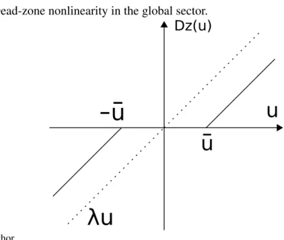
Figure 8 – Dead-zone nonlinearity in the global sector. . . 44

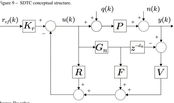
Figure 9 – SDTC conceptual structure. . . 47

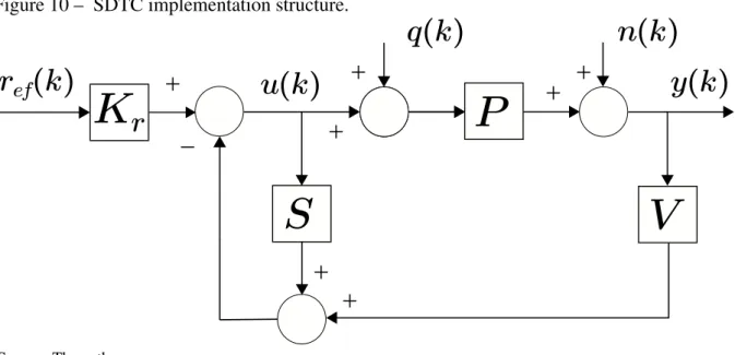
Figure 10 – SDTC implementation structure. . . 50

Figure 11 – Anti-windup SDTC scheme. . . 50

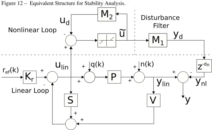
Figure 12 – Equivalent Structure for Stability Analysis. . . 53

Figure 13 – Simulation results for Example 1 (no uncertainties), Z&J is Zhang and Jiang (2008). . . 68

Figure 14 – Simulation results for Example 1 (20% dead-time uncertainty), Z&J is (ZHANG; JIANG, 2008). . . 68

Figure 15 – Simulation results for Example 1 (no uncertainties). . . 69

Figure 16 – Simulation results for Example 1 (5% dead-time uncertainty). . . 70

Figure 17 – Simulation results for Example 2 . . . 72

Figure 18 – Time varying delay for Example 2. . . 72

Figure 19 – Simulation results for Example 3. . . 74

Figure 20 – Nonlinear and linear components of the AWSDTC output - Example 3. . . . 74

Figure 21 – L₂gain dependence on set-point tracking poles - Example 3. . . 75

Figure 22 – Picture of the neonatal intensive care unit. . . 76

Figure 23 – Experimental results: Temperature control of a NICU. . . 77

Figure 24 – Decoupling between linear and nonlinear loops - simplified generic case. . . 86

AWSDTC Anti-windup Simplified Dead-time Compensator DTCs Dead-time Compensators

FOPDT First Order Plus Dead-time FSP Filtered Smith Predictor LMI Linear Matrix Inequality MIMO Multiple-input Multiple-output MPCs Model-based Predictive Controllers NCSs Networked Control Systems

NICU Neonatal Intensive Care Unit PI Proportional Integral

PID Proportional Integral Derivative SDTC Simplified Dead-time Compensator SISO Single-input Single-output

SOPDT Second Order Plus Dead-time SP Smith Predictor

⋆ Symmetric blocks in the expression of a matrix.

Z The set of integer numbers.

Z+ The set of nonnegative integer numbers. N The set of natural numbers.

R The set of real numbers. N The set of natural numbers.

k Discrete-time sample.

t Continuous time.

u Input of a system. y Output of a system.

γ L₂gain.

A⊺ The transpose of matrixA. A−1 The inverse of matrixA.

A>0 Means that matrixAis positive definite. A≥0 Means that matrixAis positive semidefinite. A<0 Means that matrixAis negative definite. A≤0 Means that matrixAis negative semidefinite.

diag(A1,A2, ...,Am) Denotes the block-diagonal matrix formed with matrices Ai,i=

1, ...,m.

col{x1,x2} Denotes the column vector

h x⊺₁ x₁⊺

1 INTRODUCTION . . . 15

1.1 Time-delay systems . . . 15

1.2 Actuator Saturation . . . 15

1.3 Related Work . . . 17

1.4 The Present Work . . . 18

1.5 Outline. . . 18

2 THEORETICAL PRELIMINARIES . . . 20

2.1 Linear Matrix Inequalities . . . 20

2.1.1 Fundamentals of LMIs . . . 20

2.1.1.1 Congruence Transformation . . . 22

2.1.1.2 Change of Variables . . . 22

2.1.1.3 Schur Complement . . . 23

2.1.1.4 S-Procedure . . . 24

2.2 Lyapunov Stability of Discrete-Time Linear Systems . . . 25

2.2.1 Stability of Systems without Delay . . . 26

2.2.2 Delay-Dependent Stability . . . 28

2.2.2.1 Lyapunov-Krasovskii Method . . . 30

2.2.2.1.1 Discrete-Time Descriptor System Review . . . 31

2.2.2.1.2 Interval Time-Varying Delay . . . 33

2.2.3 Robust Stability with Model Uncertainties . . . 36

2.2.3.1 Polytopic uncertainty . . . 36

2.2.3.2 Norm-bounded uncertainty . . . 37

2.3 Stability of Systems with Actuator Saturation . . . 39

2.3.1 Fundamentals . . . 39

2.3.2 Global Stabilization . . . 41

3 THE SIMPLIFIED DEAD-TIME COMPENSATOR . . . 46

3.1 Review of the Simplified Dead-Time Compensator (SDTC). . . 46

3.1.1 Tuning of the primary controller . . . 47

3.1.2 Tuning of the robustness filterV(z) . . . 48

3.2 The Anti-windup SDTC (AWSDTC) . . . 49

4.2 Robust Stability Analysis . . . 57

4.2.1 Equivalent State-Space Delay Representation . . . 58

4.2.2 Robust stability of the SDTC with time-varying delay . . . 60

4.2.2.1 Case 1 - SDTC with time-varying process delay . . . 60

4.2.2.2 Case 2 - SDTC with time-varying process delay and polytopic uncertainties. 60 4.2.2.3 Case 3 - SDTC with time-varying process delay and norm-bounded uncertainties 61 4.2.3 Robust stability of the AWSDTC with time-varying delay . . . 61

4.2.3.1 Case 4 - AWSDTC with time-varying process delay . . . 61

4.2.3.2 Case 5 - AWSDTC with time-varying process delay and polytopic uncertainties 63 4.2.3.3 Case 6 - AWSDTC with time-varying process delay and norm-bounded uncer-tainties . . . 64

5 RESULTS . . . 66

5.1 Simulation Results . . . 66

5.1.1 Example 1 - Comparison with other anti-windup controllers . . . 66

5.1.2 Example 2 - Robust stability analysis . . . 70

5.1.3 Example 3 - Comparison with regular SDTC andL_{2gain analysis} . . . . 73

5.1.4 Remarks on Stability . . . 75

5.2 Experimental Data . . . 76

6 CONCLUSION . . . 79

6.1 Recommendations for Future Work. . . 79

BIBLIOGRAPHY . . . 80

1 INTRODUCTION

1.1 Time-delay systems

Time-delay appears in a wide variety of real-word processes from biology to eco-nomics and communication systems. The source of delay can be related to many causes such as mass or energy transportation in the process. For instance, in the case of economics, time-delay looks quite natural since there exists time intervals between information acquisition, decision making and their effects in the market.

Time-delay can appear either in the state, control input or in the measured plant output, and is usually associated to a source of instability in the closed-loop. Therefore, stability analysis of control structures for such systems is of theoretical importance. Systems with constant delay have received most of the attention in the last decade, whereas the problem of time-varying delay started to gain more importance in recent years due to the rise of Networked Control Systems (NCSs).

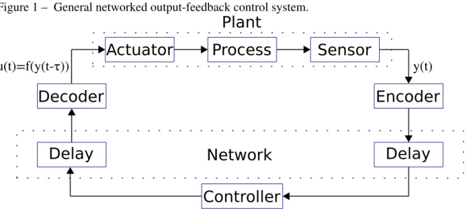
Networked control systems are distributed systems in which data is transmitted between actuators, sensors and controllers through communication networks, often relying on protocols such as Transmission Control Protocol (TCP). This research area is identified as a key for the future of control systems (LAMNABHI-LAGARRIGUEet al., 2017; HESPANHAet al., 2007) due to its diverse application; networks of mobile vehicles, smart grids and the healthcare industry are a few examples. A general structure of a networked output-feedback control system is depicted in Figure 1, wherey(t)is the process measured output,u(t)is the plant input andτ is a time-varying delay due to the communication network.

1.2 Actuator Saturation

Figure 1 – General networked output-feedback control system.

Process

Actuator

Sensor

Encoder

Decoder

Delay

Delay

Controller

Network

u(t)=f(y(t-

τ

))

Plant

y(t)

Source: The author.

undesirable consequences in the control loop, as contextualized as follows.

Windup occurs when the model of the saturation to the plant input is unknown, thus leading the states of the controller to be wrongly updated (KOTHAREet al., 1994) and causing major problems to the control system. Especially, this can make the output of the plant oscillatory or unstable. In other cases, the set-point tracking response can become painfully slow. The origin of the term windup comes from the cases of Proportional Integral (PI) and Proportional Integral Derivative (PID) controllers, in which the integral state "winds up" to large values during saturation events; the associated energy is later dissipated, causing the problems described above. It is import to note that although early practice control engineers associated this phenomenon to integral action, it was latter discovered that slow or unstable modes in the control system can also cause windup problems.

1.3 Related Work

Dead-time Compensators (DTCs) have been widely studied for about the past 25 years mainly due to their ability to improve the performance of classical PI and/or PID controllers when the process presents time-delay between the input and output. The first DTC was proposed in Smith (1957), also known in literature as the Smith Predictor (SP). The proposal presented limitations, since its application is restricted to open-loop stable plants, while the disturbance rejection response is dominated by the slow poles of the plant (NORMEY-RICO; CAMACHO, 2007). Since then several extensions have been proposed to improve robustness, disturbance rejection, and measurement noise attenuation. Some works intended to improve the SP robustness and disturbance rejection of stable and/or integrative dead time processes can be found in Astrom et al. (1994), Mataušek and Mici´c" (1996), Mataušek and Mici´c (1999), Rao et al. (2007), Kaya (2003), Rao and Chidambaram (2008), Normey-Rico and Camacho (2008), Kirtania and Choudhury (2012). Nevertheless, the study of the effect of the measurement noise is less common. In Garcíaet al.(2006), Albertos and García (2009), García and Albertos (2008) the noise effect in DTC structures is shown using simulations. In Santoset al.(2010), an analysis for stable, integrative and unstable dead-time processes using the Filtered Smith Predictor (FSP) with improved noise attenuation was presented. However, the aforementioned works are not concerned with actuator saturation, which is common in practical applications and can cause windup problems due to differences between the controller output and the actual plant input. An applicable solution of the modified Smith predictor (MATAUŠEK; MICI ´C", 1996; MATAUŠEK; MICI ´C, 1999), with anti-windup was proposed in Mataušek and Ribi´c (2012), although an optimization procedure is necessary to define some desired robustness and noise sensitivity constraints.

In Zhang and Jiang (2008) and Fleschet al.(2017) anti-windup structures for the FSP were proposed. In Huba (2013) a predictive disturbance observer based filtered PI control for First Order Plus Dead-time (FOPDT) processes is presented and in Huba (2015) the tuning for integrative plants with dead time based on robustness and performance criteria is analysed. Another alternative to deal with constraints lies in the use of Model-based Predictive Controllers (MPCs) (CAMACHO; BORDONS, 2004; NORMEY-RICO; CAMACHO, 2007). However, in the MPC case a constrained quadratic problem needs to be solved at each sampling time.

controller is free from integral action, differently from the traditional FSP, and ensures good trade-off among disturbance rejection, robustness, and noise attenuation. The results were better than those proposed by Santos et al.(2010). In Huba and Tapak (2011), a control structure equivalent to that of Torricoet al.(2013) (with addition of anti-windup action) was presented. Nevertheless, the tuning of the proposed structure was limited for open-loop stable systems only. In Torricoet al.(2016), the results obtained in Torricoet al.(2013) were extended to the case of multiple-delay Single-input Single-output (SISO) systems of any model order, namely Simplified Dead-time Compensator (SDTC). Despite of the good results in the presence of nonlinearity saturation, stability of the proposed scheme was not studied.

1.4 The Present Work

In this thesis the anti-windup characteristics of the SDTC are further studied, while stability and performance are analysed using LMI theory. Simulation results are used to analyse the tuning and establish a fair comparison with other anti-windup DTC presented in Zhang and Jiang (2008), Fleschet al.(2017) and also a constrained MPC. Furthermore, in order to test the applicability of the proposed controller, an experiment was performed to control the temperature in a Neonatal Intensive Care Unit (NICU). This work has the following specific objectives:

• To proof the nominal stability of the SDTC in the presence of actuator saturation. • To proof robust stability of the SDTC under actuator saturation for the cases of

norm-bounded and polytopic uncertainties in the process fast-model. In addition to these uncertainties, to consider the process delay to be unknown, bounded, and possibly time-varying, which can be even more harmful than constant delays. • To use simulations to establish useful rules for the tuning of the anti-windup

SDTC and demonstrate the good performance of the control structure by com-parison with other anti-windup strategies.

• To use an experimental result to prove the real-life usefulness of the anti-windup SDTC.

1.5 Outline

The rest of this thesis is organized as follows.

and performance conditions in the presence of actuator saturation are presented. To comply with this goal, basic knowledge in LMIs manipulation is initially constructed. Subsequently, concepts on the Lyapunov stability of linear systems with and without delays are presented. The final Section of the Chapter is devoted to present essential concepts on the stability of systems with actuator saturation. • Chapter 3 starts with a review of the SDTC structure. Later, its anti-windup

characteristics are explained and the structure is extended to the anti-windup SDTC (AWSDTC) case by means of a simple addition to the control structure. • Chapter 4 is a collection of nominal and robust stability results given in the form

of corollaries. Thorough proof of such statements are constructed throughout the text under the LMI framework.

• Results are presented in Chapter 5, with simulation examples showing the ef-fectiveness of the Anti-windup Simplified Dead-time Compensator (AWSDTC) structure. Experimental data for the temperature control of a neonatal incubator are discussed.

2 THEORETICAL PRELIMINARIES

In this Chapter, the preliminary knowledge necessary to proof stability of the SDTC under actuator saturation is constructed. Initially, the main properties in LMIs manipulation are presented in Section 2.1. In order to access stability, the Lyapunov stability of linear systems and the sector boundness condition for the stability of systems with actuator saturation are presented in Sections 2.2 and 2.3, respectively. Section 2.3 also presents the definition of the L₂ gain, which is used as a performance indicator of the anti-windup strategy.

2.1 Linear Matrix Inequalities

A wide variety of control problems can be described in the format of LMIs. These are matrix inequalities which have an affine relationship with a set of matrix variables. While most of the earlier works on Lyapunov stability were formulated using algebraic Riccati equations, the use of LMIs became popular in the 1990’s due to the development of efficient interior point method algorithms. LMIs soon became a powerful tool in robust control synthesis in the presence of structured uncertainties (CHILALI; GAHINET, 1996), and later in the presence of actuator saturation (WESTON; POSTLETHWAITE, 2000). There exist many packages which provide solutions to LMIs by using convex optimization, such as the Yalmip toolbox (LOFBERG, 2004).

The main attractions for the use of LMI are listed as (SKOGESTAD; POSTLETH-WAITE, 2005)

• LMIs can be used to solve problems which involve several matrix variables. • Their manipulation is flexible, thus a wide variety of problems can be posed as

LMIs in a very straightforward way.

• Restrictions that cause traditional formulations to either fail or struggle to find a solution can often be removed by using LMIs. Furthermore, LMIs can aid their extension to more general scenarios.

• Many control problems can be united into a single LMI.

2.1.1 Fundamentals of LMIs

Definition 2.1.1 A linear matrix inequality (LMI) is described by the following expression (BOYD et al., 1994)

F(x),F₀+

m

∑

i=1

xiFi>0. (2.1)

Where

• Fi=Fi⊺∈Rnxnare real given symmetric matrices.

• x= [xi, ...,xm]∈Rmis the decision variable.

• The inequality >0 denotes that F(x) is positive definite, i.e. all eigenvalues are positive. Thus, u⊺F(x)u>0for all u∈Rn_,u6=0. Non-strict LMIs are defined by

using the symbol≥0.

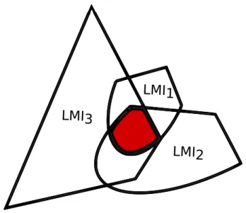
The LMI problem in Equation (2.1) is to find x such that F(x) holds. This is a convex constraint onx, i.e., the set{x|F(x)>0}is convex. Multiple LMIsF1(x)>0,F2(x)>

0, ...,Fm(x)>0,can be expressed as a single LMI of the form:

F(x) = 

   

F1(x) · · · 0

... . .. ... 0 · · · Fm(x)



   

>0, (2.2)

which is also a convex set, as illustrated in Figure 2. Figure 2 – Convex set of LMIs.

LMI1

LMI2

LMI3

Source: The author.

finding anyxf eassuch thatF(xf eas)>0 holds or determining that the problem is infeasible. The

second is called an optimization problem (also called eigenvalue problem). This consists of minimizing (or maximizing) some convex cost function of the unknown variablexsubject to LMI constraints as

minΓ(x)such thatF(x)>0. (2.3)

Important tricks used in the manipulation of LMIs (useful for the stability proofs provided in this work) are explained in the rest of this section.

2.1.1.1 Congruence Transformation

Consider a real positive definite matrixP∈Rnxn. It is known that pre- and

postmul-tiplication ofPby a full rank matrixW ∈Rnxn, and its transpose, does not affect the definitess of

P. Then, the following Equation illustrates the process of congruence transformation

W PW⊺>0. (2.4)

This trick is often used along with change of variables to eliminate nonlinearities in matrix inequalities, as illustrated in Example 1.

2.1.1.2 Change of Variables

Consider the Example 1 to explain the tricks of change of variable and also congru-ence transformation.

Example 1 Consider the problem of finding a state-feedback matrix such that the continuous closed-loop system

˙

x= (A+BK)x (2.5)

with A∈Rnxn _{and B∈}Rnxm_{is asymptotically stable. Then the standard Lyapunov LMI problem}

to make such guarantee is defined as (see Zhou et al. (1996)) to find state-feedback matrix K∈Rmxn _{and a positive definite matrix P∈}Rnxn _{such that}

Note that this problem is not linear due to the products between decision variables P and K. First, it is needed to apply a congruence transformation by multiplying both sides of each term in(2.6)by Q=P−1, obtaining

QA⊺+AQ+QK⊺B⊺+BKQ<0. (2.7)

This new matrix inequality is still nonlinear due to the product between K and the new variable Q. A change of variable L=KQ is then used to obtain

QA⊺+AQ+L⊺B⊺+BL<0, (2.8)

which is now an LMI with new variables Q>0and L∈Rmxn_{. Finally, the state-feedback matrix}

K is found after solving(2.8)by making K=LQ−1. If it is also desirable, the Lyapunov matrix P can be found by making P=Q−1.

2.1.1.3 Schur Complement

Schur Complement is a tool used mainly to eliminate quadratic terms in matrix inequalities. The Schur Complement Lemma is stated as follows

Lemma 2.1.1 Consider the following matrix inequality



Q(x) S(x) S(x)⊺ R(x) 

>0, (2.9)

where Q(x) =Q(x)⊺, R(x) =R(x)⊺, and S(x)are matrices affine in x. Then the conditions

R(x)>0and Q(x)−S(x)R(x)−1S(x)⊺>0 (2.10)

are equivalent to(2.9).

Example 2 illustrates the use of Lemma 2.1.1.

Example 2 Consider the following matrix inequality 



AA⊺ 0 0 γ2I



where scalarγ >0∈R_{is the decision variable. The inequality in Equation 2.11 is not an LMI}

because of the quadratic term inγ. To rectify this, first divide Equation(2.11)byγ



A

1 γA⊺ 0

0 γI 

>0. (2.12)

Then, rewrite Equation(2.12)as follows



 0 0 0 γI



− 

 A 0 

 h

−1 γ

i h A⊺ 0

i

>0, (2.13)

and use Lemma 2.1.1 to obtain the following LMI



   

0 0 A

0 γI 0 A⊺ 0 −γI



   

>0, withγ >0. (2.14)

2.1.1.4 S-Procedure

The S-Procedure is a method that allows two or more inequalities to be combined into only one. This is specially useful when it is necessary to guarantee that a quadratic function is negative whenever other quadratic forms are positive (or negative).

Definition 2.1.2 Let F0(x), ...,Fm(x) be quadratic functions of x∈Rn such as (BOYD et al.,

1994)

Fi(x),x⊺Aix+2u⊺_ix+b0, where Ai=A⊺_i,i=0, ...,m. (2.15)

If there existτ1≥0, ...,τm≥0such that

for all x, F0(x)− m

∑

i=1

τiFi(x)≥0, (2.16)

then it holds that

Example 3 Suppose that the following constraints on P and W hold, where x=hx⊺₁ x⊺₂ i⊺

,

x⊺ 



A⊺P+P⊺A PB

⋆ 0



x<0 (2.18)

x⊺ 



0 −CW

⋆ −2W



x≥0 (2.19)

Then, by applying Definition 2.1.2, inequalities Equations(2.18)and(2.19)can be combined into a single inequality as

x⊺ 



A⊺P+P⊺A PB−CWτ

⋆ −2Wτ



x<0, with τ>0. (2.20)

Sinceτ only appears adjacent to W , it is possible to apply the change of variable Wτ=V . Thus, the following LMI in P>0and V >0is obtained





A⊺P+P⊺A PB−CV

⋆ −2V



<0. (2.21)

2.2 Lyapunov Stability of Discrete-Time Linear Systems

In this Section the fundamentals for stability analysis of the SDTC are constructed. As it will be demonstrated in Chapter 4, stability of the closed-loop system in the nominal case (when there are no uncertainties in the process model) depends upon the process fast-model. Thus, the Lyapunov criterion for the stability of systems without delay is reviewed in Subsection 2.2.1.

2.2.1 Stability of Systems without Delay

There are different forms of stability, being input-output stability and stability of equilibrium points the most used. The latter, which is used in this work, is characterized in the sense of Lyapunov functionals. An asymptotically stable equilibrium point is a point for which the trajectories of states with different initial conditions converge as time approaches infinity (KHALIL, 2002). The region of attraction of an equilibrium pointx∗is the set of initial conditions x0 for which x(x0,t)→x∗ as t goes to infinity (BRIAT, 2015). Furthermore, an

equilibrium point is said to be globally stable if its region of attraction is the whole space, e.g.

Rn. Note that in the discrete-time domain, the time_t dependence is usually replaced by the

samplek.

In order to establish the stability of discrete-time linear systems without delay, the following Lyapunov condition is given

Theorem 2.2.1 For a chosen positive definite function V(x(k)) = xT(k)Px(k), ∀x6= 0, the discrete-time system x(k+1) = f(x(k))is stable if and only if

∆V(x(k)),V(x(k+1))−V(x(k))<0, with P=P⊺>0. (2.22)

Note that Theorem 2.2.1 is in the form of a feasibility problem. It states that if there can be found any positive definite symmetric matrixPfor which∆V(x(k))<0 holds, then the systemx(k+1) = f(x(k))is stable. This kind of problem can usually be solved in a very strait manner by using LMIs. The stability phenomena is illustrated in the example that follows.

Example 4 Consider the following second-order discrete-time system

x(k+1) = 

2 0 1 3 

x(k) + 

1 1 

u(k). (2.23)

From classical control systems theory, the open-loop is unstable since the eigenvalues of A (3 and 2) are outside the unit circle. Consider then the problem of finding a stabilizing state feedback control law u(t) =−Kx; this substitution leads to the following equivalent closed-loop system

First, apply theorem 2.2.1 to Equation(2.24)as follows

V(x(k+1))−V(x(k)) =x(k)⊺(A−BK)⊺P(A−BK)x(k)−x(k)⊺Px(k)>0, P>0. (2.25) Then, by rearranging(2.25)one obtains

x(k)⊺h(A−BK)⊺P(A−BK)−P i

x(k)<0, P>0, (2.26)

which is equivalent to simply

h

(A−BK)⊺P(A−BK)−P i

<0, P>0. (2.27)

Next, apply the Schur complement Lemma to(2.27)to obtain



−P A

⊺_+K⊺_B⊺

⋆ −P−1



<0, P>0. (2.28)

By applying a congruence transformation with diag(P−1,I), and making the change of variable Q=P−1it is obtained



−Q QA

⊺_+QK⊺_B⊺

⋆ −Q



<0, Q>0. (2.29)

Finally, by setting K=NQ−1one obtains the following LMI.



−Q QA

⊺_+N⊺_B⊺

⋆ −Q



<0, Q>0. (2.30)

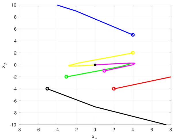
Next, consider that the LMI in Equation(2.30)was solved and the stabilizing state-feedback gain K =h−0.93 2.97iwas found. Closed-loop system(2.24)is now asymptotically stable with globally stable equilibrium point x∗=0, i.e. ∀x0∈R2, x(x0,k)→x∗ as k→inf,

since the eigenvalues of(A−BK)(0.3 and 0.8) are inside the unit circle. Figure 3 illustrates a plot of part of the region of attraction using different initial conditions for states x1and x2. Since

the system is globally asymptotically stable, the region of attraction is the wholeR2_{space. The}

Figure 3 – Convergent trajectories for equilibrium point in Example 4. Equilibrium point (x∗_{=0); initial conditions (o).}

-10 -5 0 5 10

x

1 -4

-3 -2 -1 0 1 2 3 4 5

x 2

Source: The author.

2.2.2 Delay-Dependent Stability

In this Subsection, bases for the stability investigation of the SDTC with model uncertainties are established. As it will be seen in Chapter 4, the equivalent state-space closed-loop representation of the SDTC in the presence of model uncertainties is a system with delayed states. Furthermore, the delay in the states is equal to the delay of the process model. In this work, the delay in the controlled process is considered to be not only uncertain but also possibly time-varying.

Figure 4 – Example 4 - time responses for six different initial conditionsx₀.

0 1 2 3

t -10 0 10 x x o=[-5;-4]

0 1 2 3

t -20

0 20

u

0 1 2 3

t -20 0 20 x x o=[4;5]

0 1 2 3

t -20

0 20

u

0 1 2 3

t -20 0 20 x x o=[2;-4]

0 1 2 3

t -20

0 20

u

0 1 2 3

t -5 0 5 x x o=[-3;-2]

0 1 2 3

t -10

0 10

u

0 1 2 3

t -5 0 5 x x o=[4;2]

0 1 2 3

t -10

0 10

u

0 1 2 3

t -5 0 5 x x o=[1;-1]

0 1 2 3

t -5

0 5

u

Source: The author.

2.2.2.1 Lyapunov-Krasovskii Method

Consider the following discrete-time linear system with time-varying delay

x(k+1) =Ax(k) +Adx(k−τk), k∈Z+, τk∈N, 0≤τk≤h1. (2.31)

For simplicity, denote x_k(j),x(k+ j), j=−h1, ...,0.Whenτk=h1(worst case), the initial

condition for (2.31) should be given as

col{x(0),x(−1), ...,x(−h)}=col{φ(0),φ(−1), ...,φ(−h)}. (2.32)

Then, consider the following Lemma borrowed from Fridman (2014a).

Lemma 2.2.1 If there exist positive numbers α,β and a functional V :Rn_{×. . .×}Rn

| {z }

h1+1times

→R+

such that for all k=0,1,2. . .

0≤V(xk)≤β{maxj∈[−h,0]|x(k+j)|2} (2.33)

and

V(xk+1)−V(xk)≤ −α|x(k)|2 (2.34)

for x(k)satisfying(2.31), then(2.31)is asymptotically stable.

Proofof Lemma 2.33 comes directly from Fridman (2014a), page 248, and is shown in the sequence. From (2.34) it follows that

k

∑

j=0

V(xj+1)−V(xj)≡V(xk+1)−V(x0)≤ −α k

∑

j=0

|x(j)|2. (2.35)

Then, due to (2.33), forx(k)satisfying both (2.31) and (2.32), it is obtained that

|x(k)|2≤

k

∑

j=0

|x(j)|2≤ 1

αV(x0)≤ β

αmaxj∈[−h,0]|φ(j)|

which implies that|x(k)|2is small for small enough maxj∈[−h,0]|φ(j)|2. Furthermore,

inf

∑

j=0

|x(j)|2≤ 1

αV(x0)<inf. (2.37)

Hence,|x(j)|2→0 for j→inf, and the proof is complete.

Thus, the problem of providing stability proof for systems with delayed states can also be solved by choosing an appropriate Lyapunov functional V(x), as stated by Lemma 2.2.1. Note that this condition is sufficient only, meaning that the choice of functional and its consequent manipulation can lead to more or less conservative results. This is a hot field of research, with many works published in the last ten years. For more details, see the works of Zhu and Yang (2008), Zhanget al.(2008), Shao and Han (2011), Liu and Zhang (2012) and Seuretet al.(2015).

In this work, some precautions are taken in order to yield less conservative re-sults, such as employing the convex analysis of Park et al.(2011) and thedescriptor model transformation, introduced in Fridman (2001). Thedescriptor model transformationmakes it possible to analyze systems with fast-varying delays. The employment of the convex analysis approach will be exemplified in the derivation of stability results, whereas the discrete-time model transformation from Fridman (2014a) is reviewed in the following text.

2.2.2.1.1 Discrete-Time Descriptor System Review

The introduction of the descriptor method was mainly motivated by the conservatism of prior results in time-varying delay systems. The first Lyapunov-Krasovskii conditions dealt mainly with the case of slow-varying delays, while systems with fast-varying delays had to be analyzed by using system augmentation, i.e. delay-independent conditions in the form of Lyapunov-Razumikihn functionals. Consider the definition

¯

y=x(k+1)−x(k), x(k+1) =y¯−x(k). (2.38)

Then it is clear that

In order to illustrate the use of the descriptor method, first consider the case of a delay-free autonomous system given by

x(k+1) =Ax(k), (2.40)

then substitute (2.40) into (2.39) to obtain

(A−I)x(k)−y¯=0, (2.41)

which is equivalent to (2.40) in the sense of stability (FRIDMAN, 2014a). Consider the Lyapunov functional for stability of discrete-time systems without delay presented in Theorem 2.2.1. In the descriptor approach,x(k+1) =y¯−x(k)is substituted into∆V(x(k))rather than the right-hand side of (2.31), thus

∆V(x(k)) =2x⊺(k)Py(k) +¯ y¯⊺(k)Py(k)¯ . (2.42) Now, by using (2.41), it is clear that the following equation holds for free matricesP2andP3

2[x⊺(k)P₂⊺+y¯⊺(k)P₃⊺][(A−I)x(k)−y] =¯ 0. (2.43)

Then, a new stability condition by using the descriptor method is found by adding (2.42) to (2.43), yielding

∆V(x(k)) +2[x⊺(k)P₂⊺+y¯⊺(k)P₃⊺][(A−I)x(k)−y]¯ <0. (2.44) By substitution of (2.42) into (2.44), it follows that

2x⊺(k)Py(k) +¯ y¯⊺(k)Py(k) +¯ 2[x⊺(k)P₂⊺+y¯⊺(k)P₃⊺][(A−I)x(k)−y]¯ <0, (2.45)

which can be written in the LMI format as





P₂⊺(A−I) + (A−I)⊺P2 P−P₂⊺+ (A−I)⊺P3

⋆ P−P3−P₃⊺



Then, the autonomous system (2.40) is asymptotically stable if there exist matricesP>0,P2and

P3such that (2.46) is feasible. This method will be used in this work instead of the traditional

method wherex(k+1)is substituted into the Lyapunov functional. The two main advantages of using this method are described in Fridman (2014a) as

• The use of the descriptor method yields less conservative stability conditions (with or without delay).

• LMIs are easily extended for the case of uncertain systems, due to the affine relationship in the system matrices.

2.2.2.1.2 Interval Time-Varying Delay

Note that system (2.31) was defined for small like delaysτk∈[0,h1]. However, the

motivation in this work is to provide stability analysis for systems with non-small interval delays such as

x(k+1) =Ax(k) +Adx(k−τk), k∈Z+, τk∈N, h0≤τk≤h1. (2.47)

This can be achieved by considering the following Lyapunov-Krasovskii functional (FRIDMAN, 2014a)

V(x(k)) =VP(k) +VS(k) +VR(k) +VS1(k) +VR1(k) (2.48)

where

VP(k) =xTPx

VS(k) = k−1

∑

j=k−h0

xT(j)Sx(j)

VR(k) =h0

−1

∑

m=−h₀ k−1

∑

j=k+m

yT(j)Ry(j)

VS1(k) = k−h0−1

∑

j=k−h1

xT(j)S1x(j)

VR1(k) = (h1−h0)

−h0−1

∑

m=−h1

k−1

∑

j=k+m

yT(j)R1y(j)

y(j) =x(j+1)−x(j) P>0,S>0,R>0,S1>0,R1>0.

This analysis employs the discrete-time version of the Jensen’s inequality (HIEN; TRINH, 2016), which is stated in the following Lemma.

Lemma 2.2.2 For integers a<b, a functionθ :Z_[a,b]→Rn_{and a matrix R>}0, the following

inequality holds

b

∑

k=a

θ⊺(k)Rθ(k)≥ 1 l

b

∑

k=a

θ⊺(k) !

R

b

∑

k=a

θ(k) !

, (2.50)

where l=b−a+1denotes the length of interval[a,b]inZ_.

In order to find an LMI that establishes stability conditions for system in (2.47), it is necessary to find ∆V(x(k))as defined by Lyapunov functional in (2.48), (2.49). Thus, by applying suitable math to (2.49) and using the descriptor method substitution from Equation (2.38) it is found that

∆VP(k) =2xT(k)Py(k) +yT(k)Py(k) (2.51)

∆VS(k) =xT(k)Sx(k)−xT(k−h0)Sx(k−h0) (2.52)

∆VS1(k) =xT(k−h0)S1x(k−h0)−xT(k−h1)Sx(k−h1) (2.53)

∆VR(k) =h20yT(k)Ry(k)−h0 k−1

∑

j=k−h0

yT(j)Ry(j) (2.54)

∆VR1(k) = (h1−h0)2yT(k)R1y(k)−(h1−h0) k−h0−1

∑

j=k−h1

yT(j)R1y(j) (2.55)

By applying Jensen’s inequality to the summation terms in the right-hand side of equations (2.54) and (2.55), and using the reciprocally convex approach, the following relations are obtained

∆VRjen(k)≡h

2

∆VR1jen(k)≡(h1−h0)

2_yT_(k)R

1y(k)−ηT





R₁ S₁₂

⋆ R1



η≥∆VR1(k), (2.57)

where

η = 

x(k−

h0)−x(k−τk)

x(k−τ_k)−x(k−h₁) 

, and (2.58)





R1 S12

⋆ R1



≥0 for someS12. (2.59)

Then, define

∆Vtime(x(k)) =∆VP(k) +∆VS(k) +∆VS1(k) +∆VRjen(k) +∆VR1jen(k), (2.60)

which is computed as the sum of the terms in the right-hand side of equations (2.51), (2.52), (2.53), (2.56) and (2.57). Next, by applying the descriptor method to system (2.47), it is obtained

DESCuns(k)≡2[x⊺(k)P₂⊺+y¯⊺(k)P₃⊺][(A−I)x(k) +Adx(k)−y] =¯ 0. (2.61)

Finally, by addition of (2.61) to (2.60) and definition of

ηcase1(k) =col{x(k),y(k),x(k−h0),x(k−h1),x(k−τk)}, (2.62)

it is obtained that

V(x(k−1))−V(x(k))≤ηcase1(k)Tϒ11ηcase1(k)≤ −α|x(k)|2, (2.63)

Theorem 2.2.2 The closed-loop system (2.47) is asymptotically stable for all time-varying delays h0≤τk ≤h1if there exist matrices P>0,R>0,S>0,R1>0,S1>0,P2,P3,S12 such

that LMIs(2.59)and

ϒ₁₁= 

         

Ψ₁₁ Ψ₁₂ R 0 P₂TAd

⋆ Ψ₂₂ 0 0 P₃TA_d

⋆ ⋆ Ψ₃₃ S12 R−S12

⋆ ⋆ ⋆ Ψ₄₄ R₁−S₁₂T

⋆ ⋆ ⋆ ⋆ Ψ₅₅



         

≤0 (2.64)

are feasible, where

Ψ₁₁=S−R+ (AT −I)P2+P2T(A−I), Ψ₁₂=P−P₂T+ (AT−I)P3, Ψ₂₂=P+Rh2₀+R1(h1−h0)2−P3T −P3, Ψ₃₃=−R−S+S1−R1, Ψ₄₄=−S1−R1, Ψ₅₅=S12+ST12−2R1.

(2.65)

2.2.3 Robust Stability with Model Uncertainties

Model uncertainties are the differences between the actual system and its model. The less sensitive to such differences the more robust the control system is. In this Subsection, the LMI (2.64) is extended to the case of model uncertainties, which can be either structured (using polytopic representation) or unstructured (with norm-bounded matrices). Since the LMI (2.64) is affine in the system matrices, it can be applied to both of these cases.

2.2.3.1 Polytopic uncertainty

Lets denote matricesAandAd from system (2.47) with (FRIDMAN, 2014a)

Γ=hA Ad

i

, Γ∈Π{Γ_j,j=1, ...,M} (2.66)

Γ=

M

∑

j=1

ωjΓj, for some 0≤ωj≤1, M

∑

j=1

ωj=1, (2.67)

whereΓ_j=hAj A_dj i

describes theM vertices of the polytope. Then, the following corollary establishes stability of system (2.47) in the presence of polytopic like uncertainties.

Corollary 2.2.1 Assume that(2.59)and M LMIs(2.64)written in the vertices of Γ_j

ϒ₁₁j =           

Ψ₁₁j Ψ₁₂j R 0 P₂TA_dj

⋆ Ψ₂₂ 0 0 P₃TA_dj

⋆ ⋆ Ψ₃₃ S12 R−S12

⋆ ⋆ ⋆ Ψ₄₄ R1−S12T

⋆ ⋆ ⋆ ⋆ Ψ₅₅

          

≤0 (2.68)

are feasible for the same matrices P>0,R>0,S>0,R1>0,S1>0,P2,P3and S12, where

Ψ₁₁j =S−R+ (AjT _−I)P

2+P2T(Aj−I), Ψ₁₂j =P−P₂T + (AjT _−I)P

3. (2.69) Then M

∑

ωjϒ₁₁j =ϒ11<0, (2.70)

and the closed-loop system (2.47) with polytopic type uncertainties described by (2.66) and (2.67)is asymptotically stable for all time-varying delays h0≤τk≤h1.

2.2.3.2 Norm-bounded uncertainty

Consider the following system

where the norm-bounded uncertainties are of the formh∆A(k) ∆Ad(k)

i

=Eδ(k)hHA HAd

i . The matricesE,HAandHAd are constant and known, whereasδ(k)is an unknown time-varying

matrix satisfying

δT(k)δ(k)≤I. (2.72)

In order to analyse this case, first matricesAandAd are replaced inϒ11 (Equation

(2.64)) by A+Eδ(k)HA and Ad+Eδ(k)HAd, respectively. Then, separation of terms with

uncertainties leads to the following inequality

ϒ₁₁+ϒ₁₂δ(k)ϒT₁₃+ϒ₁₃δ(k)TϒT₁₂<0. (2.73) where

ϒ₁₂=           

P₂TE P₃TE 0 0 0           

, ϒ₁₃=            HA T 0 0 0 HAd T            . (2.74)

Then, by the application of the following inequality for some scalarε>0 (XIE, 1996)

ϒ₁₂δ(k)ϒT₁₃+ϒ₁₃δ(k)TϒT₁₂≤ε−1ϒ₁₂ϒT₁₂+εϒ₁₃ϒT₁₃, (2.75) and Schur complements, the following LMI is obtained



   

ϒ₁₁ ϒ₁₂ εϒ₁₃

⋆ −ε 0

⋆ ⋆ −ε



   

<0. (2.76)

Then, the following Corollary establishes robust stability of system (2.71).

Corollary 2.2.2 The system (2.71) is asymptotically stable for all time-varying delays h0≤

τk≤h1and allδ(k)satisfying Equation(2.72)if there exists matrices P>0,R>0,S>0,R1>

2.3 Stability of Systems with Actuator Saturation

2.3.1 Fundamentals

Systems with saturating actuators are on the boundary between linearity and non-linearity. Even if an open-loop process is linear, the saturation of the actuator will turn the closed-loop into a nonlinear system. Thus, in this Section, the basis for understanding how satu-ration affects stability and performance of closed-loop systems is briefly presented. The stability condition is presented using the sector nonlinearity model approach, whereas a performance condition is presented in the form of theL₂gain.

There are three main approaches to tackling the stability problem of saturating systems, namely the global, semi-global and regions of stability approaches. When saturation occurs, it may not be possible to guarantee asymptotic stability of the closed-loop system for all initials conditions. Determination of the so calledregions of stabilityis, thus, of theoretical importance for analysis of such systems. Herein, the phenomena of loss of stability for different initial conditions is illustrated by means of Example 4. However, the problem of finding ellipsoids of stability is not treated further, as this thesis concentrates in providing global stability analysis only.

Example 5 Consider the same second-order discrete-time open-loop unstable system from Example 4

x(k+1) =A= 

2 0 1 3 

x(k) + 

1 1 

u(k) (2.77)

Once again, consider a state feedback control law u(k) =−Kx(k), with K=h−0.93 2.97 i

form

x(k+1) =Ax(k) +Bsat(Kx(k)), with sat(Kx(k)) =       

     

10, if Kx(k)>10 Kx(k), if|Kx(k)| ≤10 −10, if Kx(k)<−10

(2.78)

Figures 5 and 6 show the trajectories and the time-response of the saturated system for the same initial conditions of Example 4. Note that now three of the trajectories were divergent, for x0= [−5;−4], x0= [4; 5]and x0= [2;−4]. In these cases, the system remained

saturated for almost all the time. Interestingly, for both x0= [−3;−2]and x0= [4; 2], spite of

the control getting saturated in the initial instants, the trajectories converge for the origin. It is clear that, although being asymptotically stable to the origin in the absence of saturation, the origin becomes only a regional equilibrium point in the presence of the saturation nonlinearity.

Figure 5 – Convergent and divergent trajectories in Example 5. Regional equilibrium point (x∗_{=0); initial conditions (o).}

-8 -6 -4 -2 0 2 4 6 8

x

1

-10 -8 -6 -4 -2 0 2 4 6 8 10

x 2

Figure 6 – Example 5 - time responses for six different initial conditions. 0 0.5 t -10 0 10 x x o=[-5;-4]

0 1 2 3

t -10 0 10 u 0 0.5 t -10 0 10 x x o=[4;5]

0 1 2 3

t

-10 0 10

u

0 0.2 0.4

t -10 0 10 x x o=[2;-4]

0 1 2 3

t

-10 0 10

u

0 1 2 3

t -5 0 5 x x o=[-3;-2]

0 1 2 3

t

-10 0 10

u

0 1 2 3

t -5 0 5 x x o=[4;2]

0 1 2 3

t

-10 0 10

u

0 1 2 3

t -5 0 5 x x o=[1;-1]

0 1 2 3

t

-5 0 5

u

Source: The author.

2.3.2 Global Stabilization

the following formal result can be stated

Theorem 2.3.1 A discrete-time system

x(k+1) =Ax(k) +Bu(k) (2.79)

can only be globally stabilized by means of bounded feedback control laws if and only if 1. the pair (A,B) is stabilizable;

2. all the eigenvalues of matrix A have modulus equal to or less than 1,

where system(2.79)is said to be globally asymptotically stabilizable if and only if there exists a bounded control law for which x∗=0is the global equilibrium point, i.e. for any initial condition x₀, the trajectory x(x0,k)→0as k→∞.

Consider system (2.79) with a feedback control lawu(k) =−Kx(k)and lets formally define the saturation nonlinearity model for SISO systems (since this work does not treat the case of Multiple-input Multiple-output (MIMO) systems) as

sat(u) =sign(u)×min{|u|,|u|}¯ ,u¯>0, (2.80)

Figure 7 – The saturation function.

sat(u)

u

u

u

u

u

where ¯uis the bound on the control signal. Then, the closed-loop system can be re-written as

  

 

x(k+1) =Ax(k) +Bsat(u(k)) u(k) =−Kx(k).

(2.81)

This kind of representation, however, is not interesting for the study of stability, and the following dead-zone operator is defined

Dz(u) =u−sat(u), (2.82)

thus closed-loop system (2.81) can be re-written in a equivalent manner as

  

 

x(k+1) = [A+BK]x(k) +BDz(u(k)), u(k) =−Kx(k),

(2.83)

Note that, when there is no saturation in the control signalu(k) =sat(u(k)) =0, thus the problem of stability of (2.83) is reduced back to the problem of stability of system (2.79). Therefore, the connection between a linear system and the nonlinear operatorDzis clear.

Consider now the following equations

foru≥0 :Dz(u)≥0 andDz(u)≤λu, foru≤0 :Dz(u)≤0 andDz(u)≥λu,

(2.84)

whereλ is a positive scalar. Whenλ =1, the decentralized nonlinearityDz(u)is said to belong globally toSector[0,1]. Similarly, whenλ<1 it is said thatDz(u)belongs locally toSector[0,λ]. This study focus on global stability, then from eq. (2.84) and for some one-by-one matrixW >0, the following inequality holds

2Dz(u)T_{W[u−Dz(u)]≥0. (2.85)}

Figure 8 – Dead-zone nonlinearity in the global sector.

Dz(u)

u

u

u

λ

u

Source: The author.

Example 6 Consider the problem of checking if the closed system(2.83)is globally stable for a given state-feedback matrix K. By denoting Acl=A+BK,u˜=Dz(u), and applying the Lyapunov

functional from Theorem 2.2.1

∆V(x(k)) = [x⊺(k)A⊺_cl+u˜⊺B⊺]P[Aclx(k) +Bu]˜ −x(k)⊺Px(k)<0, (2.86)

which can be written in matrix form as

 x(k) ˜ u(k)   ⊺ A ⊺

clPAcl−P A

⊺

clPB

⋆ B⊺PB

   x(k) ˜ u(k) 

<0. (2.87)

Moreover, applying the sector boundedness condition(2.85)to(2.83)

2 ˜u(k)W[−Kx(k)−u(k)]˜ ≥0, (2.88)

which can be written in matrix format as

 x(k) ˜ u(k)   ⊺ 

0 −K⊺W

⋆ −2W    x(k) ˜ u(k) 

≥0. (2.89)

By using the S-procedure, inequalities(2.87)and(2.89)can be combined as





A⊺_clPAcl−P A⊺_clPB−K⊺Wτ

⋆ B⊺PB−2Wτ



Sinceτonly appears adjacent to W, the change of variable V =Wτ can be applied, thus





A⊺_clPA_cl−P A⊺_clPB−K⊺V

⋆ B⊺PB−2V



<0. (2.91)

Finally, closed-loop system(2.83)is globally asymptotically stable if LMI (2.91)is feasible for some P>0, W >0. Note that, in this example, K was supposedly designed using conventional methods and is previously known, thus not being a decision variable in(2.91). If the project of K was the intention, tough,(2.91)would need to be further manipulated. However, the use of LMIs in this work is concerned with demonstrating stability of closed-loops in the presence of actuator saturation (and also process delay) rather than synthesizing stabilizing control laws.

In order to establish a performance indicator for the SDTC anti-windup strategy (in the nominal case) the following definition will be used throughout this work.

Definition 2.3.1 A nonlinear system with input ulin(k)and output yd(k)has anL2 gain ofγ

when

|yd|2<γ|ulin|2+θ, (2.92)

where|.|2denotes the standard Euclidean vector norm andθ is a positive constant.

3 THE SIMPLIFIED DEAD-TIME COMPENSATOR

This Chapter presents the SDTC control structure and its tuning procedures. Initially, a review of the SDTC (TORRICOet al., 2016) is presented in Section 3.1. Later, in Section 3.2, the anti-windup strategy for the SDTC (AWSDTC) is explained.

3.1 Review of the Simplified Dead-Time Compensator (SDTC)

The unsaturated SDTC control structure is depicted in Fig. 9, where Pn(z) =

Gn(z)z−dn is the nominal process, withGn(z)anddnbeing the fast model and nominal dead-time,

respectively. PlantP(z) =G(z)z−τk is the model of the real process. The input-output transfer functions for the nominal case(Pn(z) =P(z))are

Hyr(z) =

Y(z) Re f(z)

= KrPn(z) 1+R(z) +Gn(z)F(z)

, (3.1)

Hyq(z) =

Y(z)

Q(z) =Pn(z)

1− Pn(z)V(z) 1+R(z) +Gn(z)F(z)

, (3.2)

Hun(z) =

U(z) N(z) =

−V(z)

1+R(z) +Gn(z)F(z)

, (3.3)

whereU(z),Y(z), Re f(z), N(z)and Q(z)refer to the Z-transform of the control actionu(k),

process outputy(k), referencere f(k), measurement noisen(k), and input load disturbanceq(k),

respectively.

For such control strategy, robust stability is achieved if the following condition

Ir(ω) = |1+R(e

jωTs_{) +G}

n(ejωTs)F(ejωTs)|

|Gn(ejωTs)V(ejωTs)| >δP(ω), (3.4) is met, whereTsis the sampling time, 0<ω <π/Ts,δP(jω)is the norm-bounded multiplicative

uncertainty, andIr(ω)is defined as robustness index.

It is important to highlight from Equations (3.1) to (3.4) thatKr,R(z)andF(z)can

be tuned in order to obtain a desired set-point tracking, while the filterV(z)is set for: (i) to cancel the effect of slow or unstable poles for disturbance rejectionHyq(z); (ii) to obtain a desired

Figure 9 – SDTC conceptual structure.

R

F

G

_n

K

_r

-+ +

z

P

V

+

+ -+

+ + +

y(k)

r

(k)

u(k)

q(k)

n(k)

Source: The author.

3.1.1 Tuning of the primary controller

Simple tuning rules for the primary controller, defined byKr,R(z), andF(z), were

established by (TORRICOet al., 2016) in order to obtain a desired set-point tracking. Feedback polynomialsR(z)andF(z)are FIR filters

R(z) =r1z−1+r2z−2+...+rn−1z−n+1, (3.5)

F(z) = f0+f1z−1+f2z−2+...+ fn−1z−n+1, (3.6)

wherenis the order of the fast modelGn(z). Coefficients ofR(z)andF(z)are obtained by means

by solving an equation of the typeMx=y, with

2n−1                                                     

1 0 . . . 0 b1 . . . 0

a1 1 ... b2 ...

... a1 0 ... 0

an ... 1 bn b1

0 an a1 0 ...

| {z }

n−1

0 0 an

| {z }

n

0 bn

                                    r1 ...

rn−1

f0

...

fn−1

                  =                  

p1−a1

...

pn−an

pn+1

...

p2n−1

                  , (3.7)

whereMis a non-singular 2n−1 square matrix,a1. . .anandb1. . .bnare the coefficients of

Gn(z) =

b1z−1+b2z−2. . .bnz−n

1+a1z−1+a2z−2. . .anz−n

, (3.8)

and p1. . .p2n−1are the coefficients of the desired characteristic polynomial.

Note that in the case of FOPDT systems,R(z) =0 andF(z) = f0, which is a simple

gain, thus the control structure reduces to the one presented in (TORRICOet al., 2013). Kris a

gain calculated to yield zero steady-state error, then it follows that

Kr=

1+F1(1) +Gn(1)F2(1)

Pn(1)

. (3.9)

3.1.2 Tuning of the robustness filterV(z)

Robustness filterV(z)is tuned aiming: (i) to reject step-like disturbances applied in the control signal; (ii) to eliminate slow modes of the plant modelPn(z); (iii) to establish desired

compromise between robustness and disturbance rejection. Such goals can be met by applying the following filter

V(z) =b0+b1z

−1_+...+b pz−p

where pis the number of slow modes of the plant model andβ is the filter tuning parameter. For the first objective (i)Hyq(z)must be zero at steady-state, i. e.

V(1) =1+R(1) +Gn(1)F(1) Pn(1)

. (3.11)

For the second objective (ii), the poles pi of the process model must be canceled

fromHyq(z), thus

1− Pn(z)V(z) 1+R(z) +Gn(z)F(z)

z=pi6=1

=0, (3.12)

d dz

1− Pn(z)V(z) 1+R(z) +Gn(z)F(z)

z=pi=1

=0. (3.13)

Then, coefficients b0. . .bp are computed using (3.11), (3.12) and (3.13). Such

equations altogether set a linear system so that coefficientsb0. . .bpcan be readily found.

Frequency response characteristics of the objective (iii) can be met by user adjustment of 0<β <1 parameter.

3.2 The Anti-windup SDTC (AWSDTC)

It is an essential question for any anti-windup control strategy a proper knowledge of the control signal excursion in nominal operation. Within this context, it is fundamental to obtain the control law for the SDTC structure, which can be found by inspection on its block diagram presented in Figure 9, leading to

U(z) = KrRe f(z)−V(z)Y(z)

1+S(z) , (3.14)

where

S(z) =R(z) +Gn(z)(F(z)−V(z)z−d) (3.15)

Figure 10 – SDTC implementation structure.

S

K

_r

+

-+

+

P

V

+

+

+

+

y(k)

r

(k)

_u(k)

q(k)

n(k)

Source: The author.

Note that if the plant is under input saturation, the integrative and slow modes of 1+S(z)can produce the windup effect, leading the system to become oscillatory or even unstable.

Anti-windup characteristics of the SDTC is devised by simply adding the nonlinear saturation model

sat(u) =sign(u)×min{|u|,|u|}¯ ,u¯>0 (3.16) prior to the input of the plant, as illustrated in Figure 11.

Figure 11 – Anti-windup SDTC scheme.

S

K

_r

-+ +

P

V

+ +

+

y(k)

r

(k)

u(k)

q(k)

n(k)

u

(k)

In this case, the control signal is given by

U(z) =KrRe f(z)−(1+S(z))Ua(z)−V(z)Y(z). (3.17)

In order to properly analyze anti-windup characteristics of the SDTC controller, important features related to the reference tracking and disturbance rejection must be observed as following.

For such control strategy reference tracking is reached by means of Kr given in

equation (3.9), which is a simple gain computed from steady-state behavior. On the other hand disturbance rejection is guaranteed by the proper design and tuning of theV(z)robustness filter in equation (3.10).

Therefore, one may notice that neitherKr norV(z)apply integral action to

4 CLOSED-LOOP STABILITY ANALYSIS

This Chapter presents global closed-loop stability analysis of the AWSDTC structures for both nominal (in Section 4.1) and modeling uncertainty (in Section 4.2) cases. Furthermore, Section 4.2 also presents robust stability results for the unsaturated SDTC. For organization purposes, the demonstration of some content used in Section 4.1 were moved to Appendix A.

Previous studies have proven that closed-loop global stability in the presence of actuator saturation cannot be achieved by a bounded input in the case of unstable processes (SONTAG, 1984), (LASSERRE, 1993) (also see Theorem 2.3.1). In case of critically stable pro-cesses, closed loop stability can only be achieved with nonlinear control laws (TARBOURIECH G. GARCIA, 2011).

Thus, in this thesis it is assumed that all the poles of the fast model Gn(z) (for

nominal stability analysis) are within the closed unit circle, and there are no multiple poles with |z|=1. Also, it is assumed that the plantP(z) =G(z)z−τk remains stable even in the presence of modeling uncertainties (for robust stability analysis). The theoretical background necessary to establish stability conditions of the AWSDTC were presented in Chapter 2. Note that in this work the control strategy is limited to SISO systems.

4.1 Nominal Stability Analysis of the AWSDTC

In order to analyse stability and performance of the nominal anti-windup SDTC (Pn(z) =P(z)), the scheme in Fig. 11 is redrawn in a more attractive equivalent form depicted by

Fig. 12 (seedemonstrationin Appendix A), where

M1(z) = Gn(z)

1+R(z) +Gn(z)F(z)

, and (4.1)

M2(z) =−₁R(z) +Gn(z)F(z)

+R(z) +Gn(z)F(z)

. (4.2)

As it can be seen, the system is divided in three parts, namely the linear loop, the nonlinear loop and the disturbance filter, with outputy=ylin−ydz−dn. This kind of decoupled

Figure 12 – Equivalent Structure for Stability Analysis.

M

₁

M

₂

+

+

-u

_lin

y

_lin

y

_d

y

u

~

u

_d

F

z

K

_r

-+ + +

+ +

r

(k)

q(k)

n(k)

y

_nl

Source: The author.

The linear loop represents how the system would behave in the absence of control saturation. Comparing Eqs. (3.1) and (4.1) it can be seen that all the poles ofM1(z)are within

the unit circle, therefore in the nominal case stability of the structure in Fig. 11 depends only upon the stability of the nonlinear loop in Fig. 12.

In addition, performance of the anti-windup system can be measured by choosing an appropriate induced norm for the map fromulin toyd. From Fig. 12 note that the performance of

the anti-windup compensator is related to the size of the mapτpn:ulin→yd, which is measured

in terms of theL₂gain (see Definition 2.3.1). The size of this map represents how much the behavior of the system is deviated from the linear nominal system when a saturation event occurs. Assuming that keeping the behavior as close as possible to the linear nominal system is desired, it is said that the anti-windup compensator is successful when the size of this map is small enough. Finally, the disturbance filter M1(z)represents how the system recovers after

sat-uration events occurs. Note that when a satsat-uration event ends, the output of the dead-zone nonlinearity ˜ubecomes null. However, effects caused by the saturation are not instantaneously over, as the states of the disturbance filterM1(z)are not null. Therefore,M1(z)is responsible

for determining both speed and manner of recovery of the closed-loop system after saturation ceases.

ma-tricesAp,Bp,Cp,Dp. Without loss of generality, it is assumed thatDp=0, i.e. Gn(z)is strictly

proper. In addition, the state-space realization for FIR filtersRandFare given byAR,BR,CR,DR

and AF,BF,CF,DF, respectively. Then, the mappingτpn:ulin→yd is defined as (see

demon-strationin Appendix A)

τpn,

                  

x(k+1) =Ax(k) +¯ B¯u˜ ud=C¯2x(k) +D¯2u˜

yd=C¯1x(k)

˜

u=Dz(ulin−ud)

(4.3) where ¯ A=     

Ap−Bp∆DFCp −Bp∆CF −Bp∆CR

BFCp AF 0

−BR∆DFCp −BR∆CF AR−BR∆CR

     , ¯ B=     

Bp−Bp∆DR

0 BR−BR∆DR

     , ¯ C1=

h

Cp 0 0

i

, C¯2=

h

−∆DFCp −∆CF −∆CR

i ,

¯ D2=

h −∆DR

i

, ∆=hI−DR

i .

Using the Lyapunov functional from Theorem 2.2.1 and theL₂gain from Definition 2.3.1, a necessary but not enough condition for stability is written as

∆V(x(k)) +yT_dy_d−γ2uT_linu_lin<0. (4.4) Substitution ofx(k+1)andyd as defined in (4.3) leads to

(Ax(k) +¯ B¯u)˜ ⊺P(Ax(k) +¯ B¯u)˜ −x⊺(k)Px(k) +x⊺(k)C¯1⊺C1x(k)−γ2uTlinulin<0, (4.6)

and by definingz=hxT u˜TuT_lin iT

, inequality (4.6) can be written in an equivalent quadratic form as zT      ¯

ATPA¯−P+C¯1TC¯1 A¯TPB¯ 0

⋆ B¯TPB¯ 0

⋆ ⋆ −γ2I



   

z<0. (4.7)

Furthermore, from the sector boundedness condition of the deadzone (2.85), the following inequalities hold

2 ˜uTW h

ulin−ud−u˜

i ≥0, 2 ˜uTWhulin−C¯2x−D¯2u˜−u˜

i ≥0,

(4.8)

which can be written in matrix form as

zT     

0 −C¯2TW 0 ⋆ −2W(D¯2+I) W

⋆ ⋆ 0



   

z≥0. (4.9)

Using the S-procedure inequalities from Equations (4.7) and (4.9) are combined to obtain      ¯

ATPA¯−P+C¯1TC¯1 A¯TPB¯−C¯2TWτ 0 ⋆ B¯TPB¯−2Wτ(D¯2+I) Wτ

⋆ ⋆ −γ2I



   

<0. (4.10)

Since τ only appears adjacent toW, the change of variableV =Wτ is made. In

scalar does not alter its positiveness, hence it is not necessary to divide terms which containP andV byγ),

     ¯

ATPA¯−P A¯TPB¯−C¯₂TV 0 ⋆ B¯TPB¯−2V(D¯2+I) V

⋆ ⋆ −γI

     −      ¯ C₁T

0 0      h

−γ−1 i h

C1 0 0

i

<0, (4.11)

which is, by Schur complement, equivalent to

        ¯

ATPA¯−P A¯TPB¯−C¯₂TV 0 C¯₁T ⋆ B¯TPB¯−2V(D¯2+I) V 0

⋆ ⋆ −γI 0

⋆ ⋆ ⋆ −γI

       

<0. (4.12)

Note that the procedure above was executed in order to eliminate the quadratic term in decision variableγ. However, there still exists a problem with (4.12); in order to achieve an LMI format (described in Definition 2.1.1), decision variable P cannot stay between matrices ¯AT and ¯A. Therefore, Schur complement is applied once more to obtain

          

−P −C¯₂TV 0 C¯₁T A¯T

⋆ −V2(D¯2+I) V 0 B¯T

⋆ ⋆ −γI 0 0

⋆ ⋆ ⋆ −γI 0

⋆ ⋆ ⋆ ⋆ −P−1

          

<0. (4.13)

Now, it is necessary to eliminate the nonlinear termP−1from (4.13). For this, first diag(P−1,V−1,I,I,I)is used to apply a congruence transformation with (4.13), obtaining

          

−P−1 −P−1C¯2T 0 P−1C¯1T P−1A¯T

⋆ −2(D¯2+I)V−1 I 0 V−1B¯T

⋆ ⋆ −γI 0 0

⋆ ⋆ ⋆ −γI 0

⋆ ⋆ ⋆ ⋆ −P−1

          