Vol. 7, No. 5, 2016
Delay-Decomposition Stability Approach of
Nonlinear Neutral Systems with Mixed Time-Varying
Delays
Ilyes MAZHOUD
University of Tuins El Manar, National Engineering School of Tunis, Laboratory of research in Automatic
Control, BP 37, Belvédère, 1002 Tunis, Tunisia
Issam AMRI
University of Tuins El Manar, National Engineering School of Tunis, Laboratory of research in Automatic
Control, BP 37, Belvédère, 1002 Tunis, Tunisia
Dhaou SOUDANI
University of Tuins El Manar, National Engineering School of Tunis, Laboratory of research in Automatic
Control, BP 37, Belvédère, 1002 Tunis, Tunisia
Abstract—This paper deals with the asymptotic stability of neutral systems with mixed time-varying delays and nonlinear perturbations. Based on the Lyapunov–Krasovskii functional including the triple integral terms and free weighting matrices approach, a novel delay-decomposition stability criterion is obtained. The main idea of the proposed method is to divide each delay interval into two equal segments. Then, the Lyapunov– Krasovskii functional is used to split the bounds of integral terms of each subinterval. In order to reduce the stability criterion conservatism, delay-dependent sufficient conditions are performed in terms of Linear Matrix Inequalities (LMIs) technique. Finally, numerical simulations are given to show the effectiveness of the proposed stability approach.
Keywords—Neutral systems; Lyapunov–Krasovskii approach; asymptotic stability; mixed time-varying delays; nonlinear perturbations; Linear Matrix Inequalities (LMIs)
I. INTRODUCTION
Neutral time-delay appears in many fields of sciences and engineering, including neural networks, industrial, economy, chemical processes and population models. In fact, the presence of time-delay causes the instability, the oscillation, and performances’ degradation of dynamical systems. Neutral systems are a part of a specific class of infinite dimensions. Their stability study can be a complex issue. Recently, the stability problem of neutral systems has been the subject of considerable research [1-23]. Thus, several approaches of delay-dependent stability criteria have been developed for this problem.
The stability criteria of neutral systems with mixed time-varying delays can be classified into two concepts. Firstly, the delay-dependent stability which is based on the size of time-delay and it gives the upper bound of time-delay in the formulation. Secondly, the delay-independent stability class doesn’t include any information about the size of the time-delay. Indeed, the dependent is often less conservative than the delay-independent.
In order to reduce the conservatism, many researchers studied the nonlinear neutral systems stability with mixed
time-varying delays such as in [1] where authors consider the delay-dependent robust stability of uncertain neutral systems with mixed time-varying delays. In [2], I. Amri et al. have been studied a delay-dependent exponential stability condition for nonlinear neutral systems with mixed delays. They employ a delay-decomposition approach and the known free weighting matrices method.In [3], novel delay-decomposition condition of neutral systems with time-varying delays is proposed and new stability results were derived. In [4], the authors have been presented a new asymptotic stability results for nonlinear neutral system with mixed delays by using the delay-dividing approach. In [5], the exponential stability of neutral delay differential systems with nonlinear uncertainties is used. The problem of the delay-dependent robust stability criteria for neutral systems with mixed time-varying delays and nonlinear perturbations has been studied in [6]. In [7], new less conservative robust stability criteria of neutral systems with mixed time-varying delays and nonlinear perturbations are derived by using the delay method.
In this paper, the problem of asymptotical delay-decomposition stability for nonlinear neutral systems with mixed time-varying delays is investigated. By using a new augmented Lyapunov–Krasovskii functional including the triple integral terms for interval time-varying delays as well as the free-weighting matrices technique and Jensen integral inequality, new sufficient delay-dependent stability conditions have been proposed and expressed in terms of LMIs. These stability conditions can be easily solved by various convex optimization algorithms.
The remainder of this paper is organized as follows. In Section 2, the stability problem of nonlinear neutral systems is described. Some related preliminaries are also given. The main result of this paper is presented in Section 3. Numerical examples are carried out in Section 4 in orderto illustrate the proposed results. Section 5 concludes this paper.
II. PROBLEM DESCRIPTION AND PRELIMINARIES
2 1
0 1 2
( ) ( ( )) ( ) ( ( ))
( , ( ))
( , ( ( )))
( , ( ( )))
( ) ( ), ( ) ( ), max M, M , 0
x t A x t t A x t A x t h t f t x t
f t x t h t f t x t t
x t t x t t t h
(1)
wherex t
nis the state vector1 2
, , n n
A A A are constant matrices with appropriate dimensions.( ),t h t( ) are neutral and discrete time-varying delays satisfying the following equations:
0hmh t( )hM, h t( ) 1, (2) 0m( )t M, ( )t 1, (3)
The initial conditions functions
t ,
t are continuously differentiable on [ max M,hM,0]. The functions
0 , f t x t
,
1 ,
f t x t h t andf t x t2
,
t
are unknown nonlinearuncertainties satisfying f t0( ,0)0, f t1( ,0)0, f t2( ,0)0and
0 0
1 1
2 2
( , ( )) ( ) ,
( , ( ( ))) ( ( )) ,
( , ( ( ))) ( ( )) ,
f t x t x t
f t x t h t x t h t
f t x t t x t t
(4)
where 00,10, 2 0are given constants. Constraint (4) can be rewritten as follows:
2
0 0 0
2
1 1 1
2
2 2 2
( , ( )) ( , ( )) ( ) ( )
( , ( ( ))) ( , ( ( ))) ( ( )) ( ( )) ( , ( ( ))) ( , ( ( ))) ( ( )) ( ( ))
T T
T T
T T
f t x t f t x t x t x t
f t x t h t f t x t h t x t h t x t h t f t x t t f t x t t x t t x t t
(5)
For simplicity, note that:
0: 0( , ( ))), 1: 1( , ( ( ))), 2: 2( , ( ( )))
f f t x t f f t x th t f f t x t t Moreover, for dividing the each interval time-varying delay into two equal subintervals
hm,1hM
or
1hM,hM
and
m, 2 M
or
2 M, M
,two different cases for time-varying delays have been presented.Case I: h t( ), ( )t are differentiable functions, satisfying for all t0 :
hmh t( )hM and h t( ) 1,
( )
m t M
and( )t 1. (6)
Case II: h t( )is not differentiable or the upper bound of the derivative of h t( )and( )t is a differentiable function, and
( ), ( )
h t t satisfying:
( ) ,
m M
h h t h
(7)
This paper is devoted to investigate the delay-dependent stability analysis of time-varying delays system (1) satisfying (2) and (3) equations and under nonlinear perturbations inequalities (4) and (5). It aims to formulate a less conservative stability technique to estimate the upper bound for the delay interval. Before deriving the proposed stability criteria, the following lemmas are needed.
Lemma 1. [8]
For any constant matrix n n, T
R RR a scalar functionh:h t( ) and a vector valued function
: ,0 n
x h such that the following integrations are well defined, then:
1 1
0 2
2 2
( ) ( ) ( ) ( )
( ) ( ) ( ) ( )
2
t
T T
t h t
T T
h t
R R
h x s R x s ds t t
R R
R R
h
x s R x s ds d t t
R R
where 1( ) ( ) ( )
T t x t x tT T h
and 2( ) ( ) ( ) . t
T T T
t h t h x t x s ds
Lemma 2. [9]:The following matrix inequality
Q xT
S x
0,S x R x
where
T Q x Q x
,
T R x R x
and S x
depend on affine on x, is equivalent to R x
0, Q x
0 and
1 0.T Q x S x R x S x
Lemma 3. [10]: For any scalar ( )t 0 and any constant
matrix n n, T 0,
R RR the following inequality holds:
1 ( )
1 1
1
( ) ( ) ( ( )) ( ) ( )
2 ( ) ( ( )) ( ) ,
M t h t
T T T
M t h
T
M
x s R x s ds h h t t F R F t
t F x t h t x t h
where
2 1 2
1 2
0 1 2
( ) ( ) ( ( )) ( ) ( ) ( ( )) ( )
( )
( ) ( ( )) ( ) ( ) ( )
m m
M M M
T T T T T T T
m M m M
T T T
T t t h t
T T T T T
t t h t
x t x t h x t h t x t h x t x t t x t t
x t x t t x s ds x s ds x s ds f f f
and F is free-weighting matrix with appropriate dimensions.
III. MAIN RESULTS
delay-Vol. 7, No. 5, 2016 new stability criteria for interval time-varying delay system
(1).
Theorem1. In Case I, if hmh t( )1hM
11
and m( )t 2 M
21
, for given positivescalars hm,hM, m, M, , , 0, 1 and 2, the system (1) with uncertainty (5) and mixed time-varying delays satisfying(2) and(3) is asymptotically stable if there exist
symmetric positive definiten n matrices
, i 1,..,7 , j 1,..,7 ,
P Q i R j for any free matrix variables
, , , , , ( 1, 2)
a a a a a a
T Y W N X F a and scalars
0 ( 0, 1, 2)
i i
such that the following symmetric
LMI holds:
1 1 1 2 2
1 2 1
2
3
3
* ( ) 0 0 0 0
* * 0 0 0
* * * 0 0
* * * * 0
* * * * *
M m M M m M m M
h h T h Y h h W N X
R R R
R
R
R
(8) where
i j, 15 15and:
1,1 1 2 3 4 6 7 1 1 1 1
2
5 6 7 1 1 0 0
1,3 1 2 1 1
1,6 1 2
1,8 1 2
1,9 1 2
1,10 5
2
1,11 6
1
1,12 7
2
1,13 1,14 1,15 1
2 2 2
2
2
2
T T
T T T
T T T
M
M m
M m
Q Q Q Q Q Q Y Y X X
R R R F A A F
Y Y F A
X X
P F A F
F A R
R
h h
R F
2,2 3 1 1
2,3 1 2
2
3,3 2 1 1 2 2 2 2 1 1
3,4 1 2
3,8 1 2
4,4 1 2 2
1
T
T
T T T
T
T T
T
Q W W
W W
Q T T Y Y W W
T T
A F
Q T T
5,5 R4 Q7
5,7 R4
6,6 1 4 1 1 2 2
T T
Q N N X X
7,7 4 6 2 2
8,8 2 2
8,9 2 2
T
T
R Q N N
M F F
F A
8,13 8,14 8,15 2
2
9,9 5 2 2
10,10 2 2 5
2
1 2
M
F Q
R
11,11 2 2 2 6
1
12,12 2 2 2 7
2
13,13 0
14,14 1
15,15 2
2 2
M m
M m
R
h h
R
2
5 1 1 1 2 2 3 2 4
2 2 2 2 2 2
2 2
1 2
2
5 6 7
( ) ( )
( ) ( )
2 2 2
M M m M M m
M m M m
M
M Q h R h h R R R
h h
R R R
Proof. Choose a new augmented Lyapunov–Krasovskii functional as:
1 2 3 4
( ) ( ) ( ) ( ) ( )
V t V t V t V t V t (9) where
1( ) ( ) ( ),
T
V t x t P x t
1
2
2 1 2 3
( )
4 5 6
( ) ( )
7
( ) ( ) ( ) ( ) ( ) ( ) ( )
( ) ( ) ( ) ( ) ( ) ( )
( ) ( ) ,
M m
M
m
t t t
T T T
t h t h t t h
t t t
T T T
t t t t t
t T
t
V t x s Q x s ds x s Q x s ds x s Q x s ds
x s Q x s ds x s Q x s ds x s Q x s ds
x s Q x s ds
1 1
2 2
0
3 1 2
0
3 2 4
( ) ( ) ( ) ( ) ( )
( ) ( ) ( ) ( ) ( ) ,
m
M M
m
M M
h
t t
T T
h t h t
t t
T T
M m
t t
V t x s R x s ds d x s R x s ds d
x s R x s ds d x s R x s ds d
2 1
2
0 0 0
4 5 6
0
7
( ) ( ) ( ) ( ) ( )
( ) ( ) .
m
M M
m M
h
t t
T T
t h t
t T
t
V t x s R x s ds d d x s R x s ds d d
x s R x s ds d d
2 1 2
1 2
0 1 2
( ) ( ) ( ( )) ( ) ( ) ( ( )) ( ) ( )
( ) ( ( )) ( ) ( ) ( )
m m
M M M
T T T T T T T
m M m M
T T T
T t t h t
T T T T T
t t h t
x t x t h x t h t x t h x t x t t x t
t
x t x t t x s ds x s ds x s ds f f f
Then, the time derivative of V t( )along the trajectory of system (1) is given by:
V t( )V t1( )V t2( )V t3( )V t4( ) (10)
where
1( ) ( ) ( ) ( ) ( ),
T T
V t x t P x t x t P x t
2 1 2 3 4 6 7
1 1 1 2
3 4
5 5
2 6
( ) ( ) ( )
( ) ( ) (1 ( )) ( ( )) ( ( ))
( ) ( ) (1 ( )) ( ( )) ( ( ))
(1 ( )) ( ( )) ( ( )) ( ) ( )
( ) ( T T T M M T T m m T T T M
V t x t Q Q Q Q Q Q x t
x t h Q x t h h t x t h t Q x t h t
x t h Q x t h t x t t Q x t t
t x t t Q x t t x t Q x t
x t Q x t
2 ) T( ) 7 ( )
M x t m Q x t m
1
1 2
2
3 1 1 1 2 2 3
2
2 4 1
2 3 2 4 ( ) ( ) (( ) ( ) ( ) ( ) ) ( ) ( ) ( ) ( ) ( ) ( ) ( ) ( ) ( ) ( ) , M m M M m M T
M M m M
t T
M m
t h
t h t
T T
t h t
t T
M m
t
V t x t h R h h R R
R x t x s R x s ds
x s R x s ds x s R x s ds
x s R x s ds
and: 2 1 22 2 2
2 2 1 2
4 5 6
0
2 2 2
2 7 5 6 7 ( ) ( ) ( ) ( 2 2 ( ) ) ( ) ( ) ( ) 2 ( ) ( ) ( ) ( ) . M m m M M
T M M m
t T
M m
t
h t t
T T
h t t
h h
V t x t R R
R x t x s R x s ds d
x s R x s ds d x s R x s ds d
The upper bound of the integral terms in inequality V t3( )isestimated as:
1 1 2
2
1 2 3
2 4
( ) ( ) ( ) ( ) ( ) ( )
( ) ( )
m
M M M
m M
t h
t t
T T T
t h t h t
t T
M m
t
x s R x s ds x s R x s ds x s R x s ds
x s R x s ds
1 1 2 ( ) ( )1 1 2
( ) ( )
2 3 3
( ) ( ) ( ) ( ) ( ) ( ) ( ) ( ) ( ) ( ) ( ) ( ) ( ) ( ) M M m M m
t h t t t h t
T T T
t h t h t t h
t h t t t
T T T
t h t t t t
t
x s R x s ds x s R x s ds x s R x s ds
x s R x s ds x s R x s ds x s R x s ds
(11)
2 4 4 2 4 4 4 2 2 ( ) ( ) ( ) ( ) ( ) ( ) m M T t m T M m M t m Mx t R R
x s R x s ds
R R x t x t x t
(12) 2 2 2 2 2 0 5 55 2 2
5 5 2 ( ) ( ) 2 ( ) ( ) ( ) ( ) M M M T M M t
T t t
M t
t t
x t x t
R R
x s R x s ds d
x s ds R R x s ds
(13) 1 1 1 1 6 66 2 2 2
6 6 1 1 ( ) ( ) 2 ( ) ( ) ( ) ( ) ( ) ( ) ( ) m m M M m M T M m h t t h T M m h t t h M m t h t h
h h x t
R R
x s R x s ds d
x s ds R R
h h
h h x t x s ds
(14) 2 2 2 2 7 77 2 2 2
7 7 2 2 ( ) ( ) 2 ( ) ( ) ( ) ( ) ( ) ( ) ( ) m m M M m M T M m t t T M m t t M m t t x t R R
x s R x s ds d
x s ds R R
x t x s ds
(15) By using Lemma 3, an upper bound of integral term of( )
V t can be obtained as:
1
( )
1
1 2 1 1 2
1
( ) ( ) ( ) ( ( )) ( ) ( ) ( )
2 ( ) ( ( )) ( ) ,
M
t h t
T T T
M t h
T
M
x s R R x s ds h h t t T R R T t
t T x t h t x t h
(16)
1 1 1 ( ) ( ) ( ) ( ) ( ) ( )2 ( ) ( ) ( ( )) ,
t
T T T
t h t
T
x s R x s ds h t t Y R Y t
t Y x t x t h t
(17)
1 2 2 ( ) ( ) ( ) ( ( ) ) ( ) ( )2 ( ) ( ) ( ( ))
m t h
T T T
m t h t
T
m
x s R x s ds h t h t W R W t
t W x t h x t h t
(18)
2 ( ) 13 2 3
2
( ) ( ) ( ( )) ( ) ( )
2 ( ) ( ( )) ( )
M
t t
T T T
M t
T
M
x s R x s ds t t N R N t
t N x t t x t
(19)
1 3 3 ( ) ( ) ( ) ( ) ( ) ( ) tT T T
t t
x s R x s ds t t X R X t
Vol. 7, No. 5, 2016 For any matrices F F1, 2 with appropriate dimensions, the
following equation, from the system (1), verifies:
1 2 1 2 0 1 2
2x t FT( ) x t FT( ) Ax t( )A x t h t( ( ))A x t(( ))t x t( ) f f f 0 (21)
Therefore, combining Equations (10) and (21) yields:
( ) T( ) ( )
V t
t
t (22) with2 1 2
1 2
0 1 2
( ) ( ) ( ( )) ( ) ( ) ( ( )) ( )
( )
( ) ( ( )) ( ) ( ) ( )
m m
M M M
T T T T T T T
m M m M
T T T
T t t h t
T T T T T
t t h t
x t x t h x t h t x t h x t x t t x t t
x t x t t x s ds x s ds x s ds f f f
and is given in Equation (8).
By using the Schur Complement, it is clear to see that the results V t( )0holds if 0, hmh t( )1hM and
2
( )
m t M
.Thus, the system (1) is asymptotically stable according to the Lyapunov-Krasovskii theory.
Remark 1: Inspired by the previous works [2-10], some Lyapunov-Krasovskii functional including triple integral terms involving lower and upper bounds of each interval time varying delays have been improved an important role in reduction of conservatism to estimate the maximum allowable delay bound.
Theorem 2. In Case I, if 1hM h t( )hM
1 1
and 2 M ( )t M
2 1
, for given positive scalars hm, hM, m, M, , , 0, 1and2, the system (1) with uncertainty (5) and mixed time-varying delays satisfying Equations (2) and (3) is asymptotically stable if there exist symmetric positive definiten n matricesP Q i, i
1,..,7 ,
1,..,7 ,
j
R j for any free matrix variables T Y W Xa, a, a, a,
( 1, 2)
a
F a and scalarsi0 (i0, 1, 2) such that the following symmetric LMI holds:
1
1
2
1
2
3
1 1
* 0 0 0
* * 0 0
* * * 0
* * * *
M M M M
h T h Y h W X
R
R
R
R
(23) where
i j,
15 15with
1,1 1 2 3 4 6 7 1 1 1 1
2
5 6 7 1 1 0 0
1,3 1 2 1 1
1,6 1 2
1,8 1 2
2 2 2
T T
T T
T
T
T T
Q Q Q Q Q Q Y Y X X
R R R F A A F
Y Y F A
X X
P F A F
1,9 F A1 2
1,10 5
2
M
R
1,11 6
1
2
1 M
R h
1,12 7
2
1,13 1,14 1,15 1
2
1 M
R
F
2,2 1 1 1
2,3 1 2
2
3,3 2 1 1 2 2 2 2 1 1
3,4 1 2
3,8 1 2
4,4 3 2 2
1
T
T
T T T
T
T T
T
Q W W
W W
Q T T Y Y W W
T T
A F
Q T T
5,5 4 6
5,7 4
6,6 1 4 2 2
T
R Q
R
Q X X
7,7 4 7
8,8 2 2
8,9 2 2
T
R Q
Z F F
F A
8,13 8,14 8,15 2
2
9,9 1 5 2 2
F
Q
10,10 2 5
11,11 2 2 6
1
12,12 2 2 7
2
13,13 0
14,14 1
15,15 2
2
2 1
2 1
M
M
M
R
R h
R
2 2
5 1 1 1 2 2 3 2 4
2 2 2 2 2
1 2
5 6 7
(1 ) (1 )
(1 ) (1 )
2 2 2
M M M M
M M M
Z Q h R h R R R
h
R R R
Proof. Choose a new augmented Lyapunov–Krasovskii functional as:
1 2 3 4
( ) ( ) ( ) ( ) ( )
V t V t V t V t V t (24)
where
1( ) ( ) ( ),
T
V t x t P x t
1
2
2 1 2 3
( )
4 5 6
( ) ( )
( ) ( ) ( ) ( ) ( ) ( ) ( )
( ) ( ) ( ) ( ) ( ) ( )
M M
M
t t t
T T T
t h t h t t h
t t t
T T T
t t t t t
V t x s Q x s ds x s Q x s ds x s Q x s ds
x s Q x s ds x s Q x s ds x s Q x s ds
7 ( ) ( ) , M t T tx s Q x s ds
1 1 2 2 03 1 2
0
3 2 4
( ) ( ) ( ) ( ) ( )
( ) ( ) (1 ) ( ) ( ) ,
M M M M M M h t t T T
h t h t
t t
T T
M
t t
V t x s R x s ds d x s R x s ds d
x s R x s ds d x s R x s ds d
1 20 0 0
4 5 6
0 7 ( ) ( ) ( ) ( ) ( ) ( ) ( ) . M M M M M h t t T T
t h t
t T
t
V t x s R x s ds d d x s R x s ds d d
x s R x s ds d d
with 1 2 1 20 1 2
( ) ( ) ( ( )) ( ) ( ) ( ( )) ( )
( )
( ) ( ( )) ( ) ( ) ( )
M M
M M M
T T T T T T T
M M M M
T T T
T t t h t
T T T T T
t t h t
x t x t h x t h t x t h x t x t t x t t
x t x t t x s ds x s ds x s ds f f f
Then, the time derivative of V t( )along the trajectory of system (1) is given by:
1 2 3 4
( ) ( ) ( ) ( ) ( )
V t V t V t V t V t
(25) where
1( ) ( ) ( ) ( ) ( ),
T T
V t x t P x t x t P x t
2 1 2 3 4 6 7
1 1 1
2 3
4 5 5
2 6
( ) ( ) ( )
( ) ( ) (1 ( )) ( ( )) ( ( )) ( ) ( ) (1 ( )) ( ( )) ( ( )) (1 ( )) ( ( )) ( ( )) ( ) ( )
( ) ( T T T M M T T M M T T T M
V t x t Q Q Q Q Q Q x t
x t h Q x t h h t x t h t
Q x t h t x t h Q x t h t x t t
Q x t t t x t t Q x t t x t Q x t
x t Q x t
2 ) T( ) 7 ( )
M x t M Q x t M
1
1
2
2
3 1 1 1 2 2 3
2
2 4 1
2 3
2 4
( )
( ) ((
)
(
)
(
)
(
)
) ( )
( )
( )
( )
( )
( )
( )
(1
)
( )
( )
,
M M M M M M T
M M M M
t T
M M
t h
t h t
T T
t h t
t T M
t
V t
x t
h
R
h
h
R
R
R x t
x s R x s ds
x s R x s ds
x s R x s ds
x s R x s ds
1 23 1 1 1 2 2 3
2
2 4 1
( ) 2 3 ( ) 2 4 ( ) ( ) (( ) ( ) ( ) ( ) ) ( ) ( ) ( ) ( ) ( ) ( ) ( )
1 ( ) ( )
M
M
M
M T
M M M M
t T
M M
t h t
t h t
T T
t h t t
t T M
t
V t x t h R h h R R
R x t x s R x s ds
x s R x s ds x s R x s ds
x s R x s ds
and 1 22 2 2 2 2 2 2
1 2
4 5 6 7
0
5 6
7
( ) ( )
( ) ( ) ( ) ( )
2 2 2
( ) ( ) ( ) ( ) ( ) ( ) . M M M M M
T M M M M M
h
t t
T T
t h t
t T
t
h h
V t x t R R R x t
x s R x s ds d x s R x s ds d
x s R x s ds d
The upper bound of the integral terms in inequalityV t3( ) is
estimated as:
1 2
1 2 3
( ) ( )
2 4
( ) ( ) ( ) ( ) ( ) ( )
1 ( ) ( )
M M M M t h t t
T T T
t h t t h t t
t T M
t
x s R x s ds x s R x s ds x s R x s ds
x s R x s ds
1 2 ( )1 2 2
( ) ( )
3 2 4
( )
( ) ( ) ( ) ( ) ( ) ( )
( ) ( ) 1 ( ) ( )
M M
M M
t h t h t
t
T T T
t h t t h t h t
t t
T T
M
t t t
x s R x s ds x s R x s ds x s R x s ds
x s R x s ds x s R x s ds
(26) Using Jensen’s inequality, such that
22 4 4 2
2 4
4 4
( ) ( )
1 ( ) ( )
( ) ( ) M M T t M M T M M M t
x t R R x t
x s R x s ds
R R
x t x t
(27) 0 5 5 5 2 5 5 ( ) ( ) 2 ( ) ( ) ( ) ( ) M M M T M M tT t t
M t
t t
x t x t
R R
x s R x s ds d
x s ds R R x s ds
Vol. 7, No. 5, 2016
1
1 1
1 1
6 6
6 2 2 2
6 6
1
(1 ) ( ) (1 ) ( )
2 ( ) ( ) ( ) ( ) ( ) M M M M M M T M M h t
t h t h
T
M M
h t
t h t h
h x t h x t
R R
x s R x s ds d
x s ds R R x s ds
h h
(29) 2 2 2 2 2 7 77 2 2 2
7 7
2
(1 ) ( ) (1 ) ( )
2 ( ) ( ) ( ) ( ) ( ) M M M M M M T M M t t t T M M t t t
x t x t
R R
x s R x s ds d
x s ds R R x s ds
(30)By using Lemma 3, an upper bound of integral term of
( )
V t can be obtained as:
( )
1
2 2
( ) ( ) ( ( )) ( ) ( )
2 ( ) ( ( )) ( )
M t h t
T T T
M t h
T
M
x s R x s ds h h t t T R T t
t T x t h t x t h
(31)
1 1 1 ( ) ( ) ( ) ( ) ( ) ( )2 ( ) ( ) ( ( ))
t
T T T
t h t
T
x s R x s ds h t t Y R Y t
t Y x t x t h t
(32)
1
1
2 1 2
( )
1
( ) ( ) ( ( ) ) ( ) ( )
2 ( ) ( ) ( ( ))
M
t h
T T T
M t h t
T
M
x s R x s ds h t h t W R W t
t W x t h x t h t
(33)
1
3 3
( )
( ) ( ) ( ) ( ) ( )
2 ( ) ( ) ( ( ))
t
T T T
t t
T
x s R x s ds t t X R X t
t X x t x t t
(34)From Equation(5), the following inequalities hold:
2
0 0 0
2
1 1 1 1 1
2
2 2 2 2 2
( ) ( ) 0
( ( )) ( ( )) 0
( ( )) ( ( )) 0
T T
T T
T T
x t x t f f
x t t x t t f f
x t t x t t f f
(35)Further, for any scalars
i 0(�= 0, 1, 2), it follows from Equation(35), that2
0 0 0 0
2
1 1 1 1 1 1
2
2 2 2 2 2 2
[ ( ) ( ) ] 0 ,
[ ( ( )) ( ( )) ] 0 ,
[ ( ( )) ( ( )) ] 0 ,
T T
T T
T T
x t x t f f
x t t x t t f f
x t t x t t f f
(36)Therefore, combining Equations (25) and (36) yields: V t( )T( )t ( ),t (37) with
1
2
1 2
0 1 2
( ) ( ) ( ( )) ( ) ( ) ( ( )) ( ) ( ) ( ( )) ( ) ( ) ( ) ( ) M M M M M
T T T T
M M
T T T
M M
T t h T
t
T T
T
t t h
T t
T T T t
x t x t h x t h t x t h
x t x t t x t
x t x t t x s ds x s ds
t
x s ds f f f
andis given in Equation (23). By using the Schur Complement, it is clear to see that the results V t( )0holds if
0
, 1hM h t( )hM, and 2 M ( )t M.
Thus, the system (1) is asymptotically stable according to the Lyapunov-Krasovskii method.
Theorem 3. In Case II, for given positive scalars h hm, M, ,
m
M, , , 0, 1and2, the system (1) withuncertainty (5) and mixed time-varying delays satisfying Equations (2) and (3) is asymptotically stable if there exist
symmetric positive definiten n matrices
, i 1,3,..7 , j 1,..,7 ,
P Q i R j for any free matrix variables
, , , , , ( 1,2)
a a a a a a
T Y W N X F a and scalarsi0 (i0, 1, 2) such
that the following symmetric LMI holds:
1 1 1 2 2
1 2 1
2
3
3
* ( ) 0 0 0 0
* * 0 0 0
* * * 0 0
* * * * 0
* * * * *
M m M M m M m M
h h T h Y h h W N X
R R R R R R (38)
where
i j, 15 15with
1,1 1 3 4 6 7 1 1 1 1
2
5 6 7 1 1 0 0
1,3 1 2 1 1
1,6 1 2
1,8 1 2
1,9 1 2
1,10 5 2 1,11 6 1 1,12 7 2
1,13 1,14 1,15 1
2 2 2
2 2 2 T T T T T T T T M M m M m
Q Q Q Q Q Y Y X X
R R R F A A F
Y Y F A
X X
P F A F
F A R R h h R F
2,2 3 1 1
2,3 1 2
2
3,3 1 1 2 2 2 2 1 1
3,4 1 2
3,8 1 2
4,4 1 2 2
5,5 4 7
T
T
T T T
T
T T
T
Q W W
W W
T T Y Y W W
T T
A F
Q T T
5,7 4
6,6 4 1 1 2 2
7,7 4 6 2 2
8,8 2 2
8,9 2 2
8,13 8,14 8,15 2
2
9,9 5 2 2
10,10 2 2 5
2
1
1 2
T T
T
T
M
R
Q N N X X
R Q N N
M F F
F A
F
Q
R
11,11 2 2 2 6
1
12,12 2 2 2 7
2
13,13 0
14,14 1
15,15 2
2 2
M m
M m
R
h h
R
2 1 2
1 2
0 1 2
( ) ( ) ( ( )) ( ) ( ) ( ( )) ( )
( )
( ) ( ( )) ( ) ( ) ( )
m m
M M M
T T T T T T T
m M m M
T T T
T t t h t
T T T T T
t t h t
x t x t h x t h t x t h x t x t t x t
t
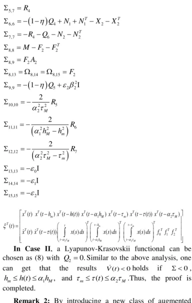
x t x t t x s ds x s ds x s ds f f f
In Case II, a Lyapunov-Krasovskii functional can be chosen as (8) with Q20.Similar to the above analysis, one
can get that the results V t( )0holds if 0,
1
( ) ,
m M
h h t h and m( )t 2 M.Thus, the proof is completed.
Remark 2: By introducing a new class of augmented Lyapunov-Krasovskii functional approach, new delay-decomposition stability criteria for nonlinear neutral systems with mixed time-varying delays are obtained in Theorems 1-3. The proposed augmented Lyapunov functional using the novel triple integral inequality is more robust than existing results in literature. It gives the upper bounds of time-varying delays
( ), ( )
h t t for the asymptotic stability of system (1) which can be provided larger stability domain. In addition, by applying free-weighting matrices and Jensen integral inequality, our decomposition approach, developed in Theorems 1-3, yields a much less conservative delay bounds and extends the feasible region of stability method for system (1).
Remark 3: In order to derive a fewer restrictive stability criteria for system (1), many free-weighting matrix variables are employed in Theorems 1-3. In fact, this technique of decision variables reduces the computational complexity of the obtained stability approach which is less than the previous methods.
Remark 4: In this work and from the practical point of
time-varying delays, chaotic systems with varying delays and neural networks systems.
IV. ILLUSTRATIVE EXAMPLES
In this section, two examples are presented in order to show the less conservatism of the elaborated stability condition and to demonstrate the effectiveness of the proposed approach.
Example 1.
Consider the following nonlinear neutral system with mixed time-varying delays, as given in [10]:
1 2
1.2 0.1 0.6 0.7 0
, , ,
0.1 1 1 0.8 0
c
A A A
c
(39)
where 0 c 00,10,and 2 0.
Case I. For c0.1, 1 0.1,
M 1, 0.5,0,2 0.2
and different values of
2,the maximal allowabledelay of hMestimated by Theorems 1 and 2 are illustrated in
Table 1. This table shows the numerical results for different values of
2,
0 0 and
0 0.1. As
2increases,M
h
decreases. In addition, the proposed stability technique gives a much less conservative result than other recent ones.
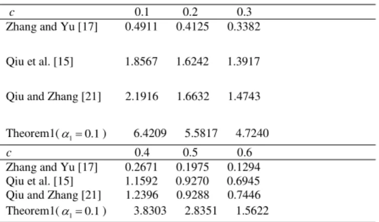
Case II. For
00.1,
10.2,
20.1, 2 0.2, 1and different values of c, the maximum admissible upper bound on the allowable time delay of hM
Mobtained fromTheorem 1 are listed in Table 2. As c increases, hMdecreases.
It is clear that the proposed stability method in this paper provides larger upper bounds of delay system than the previous results for different values of c.
Case III. For c = 0.1, 2 0.2, 1 0.1, 2 0, 0 0
and 0 0.1, and different values of ,the maximum
upper bounds on the allowable delay ofhM
Mobtained fromTheorems 1 and 2 are illustrated in Table 3. Asincreases, M
h
decreases. The presented stability criterion is less conservative than existing results.
TABLE I. MAXIMUM ALLOWABLE DELAY BOUND OFhMWITH
0.5, 0
AND DIFFERENT VALUES OF2
0 0
2
0 0.1 0.2 0.3 Rakkiyappan et al.[18] 1.4886 1.2437 0.9921 0.7367
Vol. 7, No. 5, 2016
Qiu and Zhang [21] 2.2937 1.8505 1.4565 1.1105
Theorem1(10.25) 6.0782 5.1772 3.4872 1.9325 Theorem2 (10.1) 4.7856 4.0752 2.7424 1.5156
0 0.1
2
0 0.1 0.2 0.3 Rakkiyappan et al.[18] 1.3244 1.0901 0.8475 0.6300
Lakshmanan et al.[13] 1.4440 1.1950 0.9734 0.7760
Cheng et al. [23] 1.4721 1.2466 0.9996 0.7804
Qiu and Zhang [21] 2.0417 1.6541 1.3062 0.9982
Theorem1(10.25) 5.6888 4.9444 3.4125 1.9128 Theorem2 (10.1) 4.4785 3.8915 2.6834 1.5000
TABLE II. MAXIMUM UPPER BOUND OF hM MWITH DIFFERENT
VALUES OF C
c 0.1 0.2 0.3 Zhang and Yu [17] 0.4911 0.4125 0.3382
Qiu et al. [15] 1.8567 1.6242 1.3917
Qiu and Zhang [21] 2.1916 1.6632 1.4743
Theorem1(10.1) 6.4209 5.5817 4.7240
c 0.4 0.5 0.6 Zhang and Yu [17] 0.2671 0.1975 0.1294 Qiu et al. [15] 1.1592 0.9270 0.6945 Qiu and Zhang [21] 1.2396 0.9288 0.7446 Theorem1(10.1) 3.8303 2.8351 1.5622
TABLE III. MAXIMUM UPPER BOUND OF hM MWITH DIFFERENT
VALUES OF
00 10.1 0 0.1 10.1
0 0.5 0 0.5 Chen et al. [23] 2.7423 1.1425 1.8753 1.0097 Liu [22] 2.7429 1.4462 1.8895 1.1485 Qiu and Zhang [21] 3.8066 1.6402 2.6039 1.4534 Theorem1(10.6) 8.1497 2.3438 5.6008 2.1964 Theorem2 (10.7) 5.8444 1.6738 4.0165 1.5683
Example 2.
Consider the mixed time-varying delay systems as depicted in Equation (40):
1 2
2 0.5 1 0.4 0.2 1
, , ,
0 1 0.4 1 0 0.2
A A A
(40)
with
2
0 ( , ( )) 0( , ( )) 0 ( ) ( )
T T
f t x t f t x t x t x t and
2
1 ( , ( ( ))) ( , (1 ( ))) 1 ( ( )) ( ( )).
T T
f t x t h t f t x t h t x t h t x t h t
While using the parameters 1 0.1, 2 0.2, 0,
0 0.2
,
10.1and 2 0, the upper bound of Time DelayM M
h
obtained from Theorem 3 is feasible for any delay3.8561
M
h
.
It is remarkable that this proposed criterion is much less conservative than the results shown in [14, 16].
V. CONCLUSION
This paper studied the problem of asymptotic stability for nonlinear neutral mixed time-varying delays systems. By using the Lyapunov–Krasovskii functional with triple integral terms and free weighting matrices approach, new delay-dependent stability criteria are derived by developing a delay decomposition technique. The elaborated approach is then expressed in terms of LMIs. Finally, numerical simulations have been investigated in order to show the robustness and the flexibility of the proposed stability method.
REFERENCES
[1] M.N. Alpaslan Parlakçı, Delay-Dependent Robust Stability criteria for uncertain neutral systems with mixed time-varying discrete and neutral delays, Asian Journal of Control, vol. 9, no. 4, pp. 411-421, December 2007.
[2] I. Amri, D. Soudani and M. Benrejeb, A Delay Decomposition Approach for Exponential Stability of Perturbed Neutral Systems with Mixed Delay, 7th International Multi-Conference on Systems, Signals and Devices (SSD’10), Amman, Jordan, 2010.
[3] P. L. Liu, A delay decomposition approach to stability analysis of neutral systems with time varying delay, Appl. Math. Modell, vol. 37, pp. 5013-5026, 2013.
[4] F. Qiu, B.Cui, and Y. Ji, A delay-dividing approach to stability of neutral system with mixed delays and nonlinear perturbations, Applied Mathematical Modelling, vol. 34, pp.3701-3707, 2010.
[5] Ali, MS, On exponential stability of neutral delay differential system with nonlinear uncertainties, Nonlinear Sci. Numer. Simul, vol. 17, pp. 2595-2601, 2012.
[6] J. Cheng, H. Zhu, S. M. Zhong, G. H. Li, Novel delay-dependent robust stability criteria for neutral systems with mixed time-varying delays and nonlinear perturbations, Appl. Math. Comput, vol. 219, pp. 7741-7753, 2013.
[7] Junjun HUI, Hexin ZHANG, Xiangyu KONG, and Fei MENG, A Less Conservative Robust Stability Criteria for Neutral System with Mixed Time-varying Delays and Nonlinear Perturbations, Journal of Computational Information Systems, vol. 4, no. 10, pp. 1543-1553, 2014.
[8] X.M. Zhang, Q.L. Han, A delay decomposition approach to delay-dependent stability for linear systems with time-varying delays, International Journal of Robust and Nonlinear Control, vol. 19, no. 17, pp. 1922-1930, 2009.
[9] S. Boyd, L. EL Ghaoui, E. Feron, V. Balakrishnan, Linear matrix inequalities in system and control theory, Studies in Applied Mathematics, SIAM, Philadelphia, USA, 1994.
[10] O.M. Kwon, J.H. Park, S.M. Lee, An improved delay-dependent criterion for asymptotic stability of uncertain dynamic systems with time-varying delays, J. Optim. Theory Appl., vol. 145, pp. 343-353, 2010.
[11] F. Gouaisbaut and D. Peaucelle, Delay-dependent stability of time delay systems, 5th IFAC Symposium on Robust Control (ROCOND’06), Toulouse, France, 5–7 July 2006.