ON THE ESTIMATION OF ROBUST STABILITY REGIONS FOR
NONLINEAR SYSTEMS WITH SATURATION
Daniel F. Coutinho
∗ [email protected]Daniel J. Pagano
† [email protected]Alexandre Trofino
† [email protected]∗Department of Electrical Engineering, Pontifícia Universidade Católica do Rio Grande do Sul,
Av. Ipiranga 6681, 90619900, Porto Alegre, RS, Brazil.
†Department of Automation and Systems, Universidade Federal de Santa Catarina,
PO Box 476, 88040900, Florianópolis, SC, Brazil.
ABSTRACT
This paper addresses the problem of determining robust sta-bility regions for a class of nonlinear systems with time-invariant uncertainties subject to actuator saturation. The unforced nonlinear system is represented by differential-algebraic equations where the system matrices are allowed to be rational functions of the state and uncertain parameters, and the saturation nonlinearity is modelled by a sector bound condition. For this class of systems, local stability condi-tions in terms of linear matrix inequalities are derived based on polynomial Lyapunov functions in which the Lyapunov matrix is a quadratic function of the state and uncertain pa-rameters. To estimate a robust stability region is considered the largest level surface of the Lyapunov function belonging to a given polytopic region of state. A numerical example is used to demonstrate the approach.
KEYWORDS: Nonlinear systems, stability region,
uncer-tainty, convex optimization, saturation.
RESUMO
Este artigo trata do problema de determinar regiões de
esta-Artigo submetido em 12/12/02 1a. Revisão em 03/07/03
Aceito sob recomendação do Ed. Assoc. Prof. Liu Hsu
bilidade robustas para uma classe de sistemas não lineares com incertezas invariantes no tempo e sujeitos à saturação no sinal de controle. O sistema não linear é representado por uma equação algébrico- diferencial onde as matrizes do sistema são funções racionais dos estados e incertezas e a sa-turação no controle é representada como uma condição de setor. As condições de estabilidade local propostas são ex-pressas por LMIs e estão baseadas numa função de Lyapu-nov que é polinomial (ordem 4) nos estados e quadrática nos parâmetros incertos. Para estimar a região de estabilidade robusta propõe-se um problema de maximização da maior curva de nível da função de Lyapunov dentro de um politopo dado representando as condições iniciais. Os resultados são ilustrados através de um exemplo numérico.
PALAVRAS-CHAVE: Sistemas não-lineares, região de
esta-bilidade, incerteza, otimização convexa, saturação.
1
INTRODUCTION
inequal-ity (LMI) framework. For instance, Hindi and Boyd (1998) uses the circle and Popov criteria, Gomes da Silva Jr. and Tarbouriech (1999) considers polyhedral Lyapunov functions and Johansson (2002) employs piecewise techniques. How-ever, there are few results for the nonlinear case such as the works of Barreiro et al. (2002) which combines the bifur-cation analysis and Lyapunov theory and Bean et al. (2002) which uses piecewise bilinear models and a single polyno-mial Lyapunov function.
On the other hand, the stability and performance analysis, and control synthesis of uncertain nonlinear systems has been recently addressed by many authors via convex opti-mization problems, e.g. the works of (El Ghaoui and Scor-letti, 1996; Dussy and El Ghaoui, 1997; Chesi et al., 2002) and (Trofino, 2000; Johansen, 2000; Coutinho, Trofino and Fu, 2002) that consider quadratic and polynomial Lyapunov functions, respectively. In general, non-quadratic Lyapunov functions are less conservative for dealing with uncertain nonlinear systems than the quadratic ones at the expense of extra computations Johansen (2000). Also, the LMI frame-work has some advantages over other approaches since it can handle parameter-dependent Lyapunov functions, uncertain-ties, equality and inequality constraints and so on in a numer-ical tractable way Boyd et al. (1994).
In this scenario, the purpose of this paper is to derive robust conditions in terms of LMIs for analyzing the stability of (open-loop unstable) nonlinear systems with time-invariant uncertainties and subject to input saturation based on the work of Trofino (2000) which have proposed a convex ap-proach to the domain of attraction problem for rational non-linear systems. To this end, the unforced system is described by rational differential-algebraic equations and the saturation nonlinearity is modelled by a sector bound condition. Using a polynomial Lyapunov function, we give sufficient local sta-bility conditions for the saturated systems while providing an estimate of its stability region (SR) for all possible admissi-ble uncertainty. An uncertain controlled pendulum system with input saturation is used to show the potential of our ap-proach.
The rest of this paper is as follows. Section 2 states the prob-lem of interest and Section 3 introduces some preliminary results. In the sequel, Section 4 presents the main result of this paper, Section 5 gives a numerical example and Section 6 ends the paper.
The notation used throughout this paper is standard. Rn de-notes the set ofn-dimensional real vectors,Rn×mis the set ofn×mreal matrices,Inis then×nidentity matrix,0n×m is then×mmatrix of zeros and0nis then×nmatrix of ze-ros. For a real matrixS,S′denotes its transpose, andS >0
means thatS is symmetric and positive-definite. The time
derivative of a functionr(t)will be denoted byr˙(t)and the argument(t)is often omitted. The symbol⋆for a block ma-trix represents its symmetrical block outside the main diago-nal. For two polytopesB1⊂Rn1andB2⊂Rn2the notation B1× B2represents that(B1× B2) ⊂ R(n1+n2)is a
meta-polytope obtained by the cartesian product, andV(B1× B2)
represents the set of all vertices of B1× B2 . Matrix and
vector dimensions are omitted whenever they can be inferred from the context.
2
PROBLEM STATEMENT
Consider the following nonlinear system
˙
x = f(x, τ, λ) +g(x, τ, λ, u)
0 = h(x, τ, λ)
u = sat(K′x)
(1)
wherex∈ Bx⊂Rndenotes the state,τ ∈ Bτ⊂Rldenotes the vector of algebraic variables,λ∈Rpdenotes the vector of constant uncertain parameters associated to disturbances,
u∈Ris the control input,sat(·)is the unit saturation func-tion, K ∈ Rn is a given constant vector such that system (1) is locally stable,Bxis a known polytopic region of state containing the origin, andBτrepresents the set of admissible algebraic variables. We assume for the above system that:
A1 The uncertain parameters represented byλlie in a given polytopeBλ, i.e.λ∈ Bλ.
A2 The nonlinear vectors f(x, τ, λ), g(x, τ, λ, u) and
h(x, τ, λ) are continuous on their arguments and
bounded for all(x, τ, λ)∈ Bx× Bτ× Bλ.
A3 The origin is an equilibrium point for all admissible un-certainty, i.e.f(0, τ, λ) = 0.
A4 The unit saturation function is described by
sat(K′x) =
1 K′x >1
K′x if |K′x| ≤1
−1 K′x <−1
(2)
Considering the above assumptions, the purpose of this pa-per is to analyze the local stability of the origin of system (1) while providing an estimate of its SR (stability region) in a numerical tractable manner. To this end, we will use polyno-mial Lyapunov functions which will be obtained by means of a convex optimization problem in terms of LMIs.
Lemma 1 Consider a nonlinear system x˙ = f(x, τ, λ)
where f : Bx × Bτ × Bλ 7→ Rn is a continuous func-tion such thatf(0, τ, λ) = 0. Suppose there exist positive scalarsǫ1,ǫ2,ǫ3and a continuously differentiable function
V :Bx× Bλ7→Rsatisfying the following conditions:
ǫ1x′x≤V(x, λ)≤ǫ2x′x, ∀(x, λ)∈ Bx× Bλ (3)
˙
V(x, λ)≤ −ǫ3x′x, ∀(x, τ, λ)∈ Bx× Bτ× Bλ (4)
R,{x:V(x, λ)≤1} ⊂ Bx, ∀λ∈ Bλ (5)
Then,V(x, λ)is a Lyapunov function inBx × Bλ. More-over, for allx(0) ∈ Rthe trajectoryx(t)belongs toRand approaches the origin ast→ ∞.
3
PRELIMINARIES
Before stating the main result of this paper, we introduce in the following some preliminary results in order to obtain a convex characterization of Lemma 1.
3.1
Sector Bound Condition
One way to deal with the saturation nonlinearity is to restrict the amplitude of the input signal leading to a constraint on the system state Hindi and Boyd (1998). Lettingρ ≥ 0be the allowable input amplitude over the saturation level, hereafter called the level of over saturation, the constraint
|u(t)| ≤1 +ρ
holds if and only if the system state belongs to the set
Xρ,{x:|K′x| ≤1 +ρ} (6)
Note whenρ= 0(i.e.x∈ X0) that system (1) behaves with
the following dynamics:
˙
x=f(x, τ, λ) +g(x, τ, λ, K′x), 0 =h(x, τ, λ),
and then we can apply the technique proposed in Coutinho, Bazanella, Trofino and Silva (2002) with the additional con-straintR ⊂ X0for analyzing its regional stability. However,
the state vector frequently converges to the origin from an initial point outside the setR ⊂ X0and thus the above
anal-ysis may be too conservative.
A more appropriate approach is to allow a certain level of saturation withρ > 0using the circle criterion. As a result, we have the following sector bound condition Kiyama and Iwasaki (2000):
(u−K′x)
u− 1
1 +ρK
′x
≤0, ∀x∈ Xρ (7)
Using the well-known S-procedure (Yakubovich, 1971; Boyd et al., 1994), we can add the sector condition (7) into the Lyapunov inequality (4). Thus, there exists a positive scalarµsuch that the following inequality is satisfied for all
(x, τ, λ)∈ Bx× Bτ× Bλandx∈ Xρ:
˙
V(x, λ)−µu2+ 2µρ1u′K′x−µρ2x′KK′x≤ −ǫ3x′x (8)
where
ρ1=
(2 +ρ)
2(1 +ρ) and ρ2=
1
(1 +ρ) (9)
Remark 1 The sector condition in (7) is satisfied for all
x ∈ Xρ, and thus the modified Lyapunov inequality in (8) must be tested in the meta-set(Bx∩ Xρ)× Bτ × Bλ. As a consequence, there exists a compromise betweenBxandXρ since they define the state domain in which the stability con-ditions will be checked. In other words, we have to choose the parameterρsuch that the size ofBx∩ Xρis maximized. This point will be addressed later on this Section and also in Section 5 by means of an illustrative example.
3.2
System Model Representation
Consider that the unforced system in (1) can be rewritten as indicated bellow:
˙
x = A1(x, τ, λ)x+A2(x, τ, λ)ξ
+ B1(x, τ, λ)u+B2(x, τ, λ)φ,
0 = Ω1(x, τ, λ)x+ Ω2(x, τ, δ)ξ,
0 = Φ1(x, τ, λ)u+ Φ2(x, τ, λ)φ,
(10)
where the vectorsξ ∈ Rmandφ ∈ Rq are nonlinear func-tions of(x, τ, λ), and the matricesA1(·), A2(·), B1(·), B2(·),
andΩ1(·) ∈ Rr×n,Ω2(·) ∈ Rr×m,Φ1(·) ∈ Rz,Φ2(·) ∈
Rz×qare affine functions of(x, τ, λ). Throughout this work, we may useA1(·),A2(·),B1(·),B2(·),Ω1(·),Ω2(·),Φ1(·)
andΦ2(·)without their respective dependence onx,τ,λand
t(time) in order to simplify the notation.
In order to guarantee that system (10) is well-posed, we fur-ther assume:
A5 The matricesΩ2,Φ2 in (10) have full column rank for
allx, τandλof interest.
The above assumption1 implies thatξ andφcan be
elimi-nated from (10) to recover the original system representation in (1), i.e., one can return to the original system representa-tion by definingξandφin (10) as follows
ξ=−(Ω′
2Ω2)−1Ω′2Ω1x, φ=−(Φ′2Φ2)−1Φ′2Φ1u.
1A5
Observe that the nonlinear decomposition (10) has an aug-mented space(Rn ⊆Rn+m)and the relationships between
(ξ, φ)and(x, τ, λ, u)are defined by means of the constraints
Ω1x+ Ω2ξ= 0andΦ1u+ Φ2φ= 0. As a result, the system
can only have rational nonlinearities without singularities at origin in the differential-algebraic equations (El Ghaoui and Scorletti, 1996). However, we can transform a certain differential-algebraic representation with non-rational terms into an augmented differential-algebraic form without non-rational nonlinearities. To illustrate this procedure, consider the following example.
Example 1 Consider a controlled pendulum system whose dynamics is given by
˙
x1=x2, x˙2=λsinx1−x2+u (11)
whereuis the control input andλ∈ Bλis a constant uncer-tain parameter.
Assume for above system that the anglex1 is bounded by
−π < x1 ≤π. In order to rewrite the above system in the
form (10), we define the following auxiliary variables
x3= sinx1 and τ= cosx1 (12)
With these auxiliary variables, one can construct: a differen-tial equationx˙3 =τ x2and an algebraic onex23+τ2 = 1.
Leading to the following augmented system.
˙
x1 = x2
˙
x2 = −x2+λx3+u
˙
x3 = τ x2
0 = x2
3+τ2−1
(13)
Notice in (12) that we choosex3= sinx1aiming a rational
(augmented) representation of system (11). As a result, a new differential equation have been added to the system whose dynamics depends on the algebraic variableτ= cosx1
lead-ing to a rational differential-algebraic representation as in (10) of the original system (11).
Finally, rewriting (13) as (10) give rise the following system representation
˙
x = A1x+A2ξ+B1u
0 = Ω1x+ Ω2ξ (14)
wherex= [ x1 x2 x3 ]′,ξ= [ τ x2 τ 1 ]′and
B1=
0 1 0
, A1=
0 1 0
0 −1 λ
0 0 0
, A2=
0 0 0 0 0 0 1 0 0
,
Ω1=
0 τ 0
0 0 0
0 0 x3
I3
τ I3
0 0 0
, Ω2=
−1 0 0
1 −x2 0
0 τ −1
0 0 −x
0 −x 0
0 1 −τ
.
Observe thatΩ1andΩ2as given above define the following
constraints overxandξ:
τ x2−ξ1= 0, ξ1−x2ξ2= 0, x23+τ ξ2−1 = 0,
x−xξ3= 0, τ x−xξ2= 0, ξ2−τ ξ3= 0,
whereξiare the i-th elements ofξ.
It should be noted that the trajectories of system (14) include all trajectories of the original one defined in (11). In par-ticular, suppose that x1(0), x2(0)are the initial conditions
of system (11). Then, for the initial conditionsx1(0),x2(0)
andx3(0) = sinx1(0), both systems have equal trajectories
in thex1,x2sub-space.
Remark 2 The choice of matricesA1, . . . , B2in (10) is not
unique and until now there is no a systematic way to define them. As a result, a bad choice of them can lead to a poor stability region estimate or even fail to provide the system stability (Huang and Lu, 1996). A possible way of reducing this potential conservativeness is to add free multipliers to the problem reducing the dependence on the choice of the system matrices as proposed by Huang and Jadbabaie (1999) and Trofino (2000) using different approaches. In this paper, we follow the technique of Trofino (2000) to handle state-dependent LMIs as proposed in Section 4.
3.3
Lyapunov Function Candidate
Consider the following Lyapunov function candidate
V(x, λ) =x′P(x, λ)x,
P(x, λ) =
Θ(x, λ)
In
′
P
Θ(x, λ)
In
, (15)
where P is a symmetric matrix to be determined and
Θ(x, λ)∈Rv×nis a given affine matrix function of(x, λ).
From the above definition, we can representΘ(x, λ)as fol-lows:
Θ(x, λ) =
n
X
j=1
Tjxj+
p
X
j=1
Ujλj+Y (16)
whereTj, Uj, Y are constant matrices with the same dimen-sions of Θ(x, λ), and xj, λj stand for the elements of the vectorsxandλ, respectively.
To determine the time-derivative ofV(x, λ), we need to com-pute the following term:
d(Θ(x, λ)x)
dt = ˙Θ(x, λ)x+ Θ(x, λ) ˙x (17)
Straightforwardly from (16), the termΘ(˙ x, λ)xis given by:
˙
Θ(x, λ)x=
n
X
j=1
Tjx˙jx=
n
X
j=1
where the matrixΘ(˜ x)is as follows:
˜
Θ(x) =
n
X
j=1
Tjxsj (19)
withsjdenoting thej-th row of the identity matrixIn.
Then, using (16), (17) and (18) we can obtain a convex char-acterization of (8) in terms of LMIs similarly to the procedure proposed in Trofino (2000). We make this point clear later in the proof of Theorem 2.
Remark 3 In spite of the fact thatV(x, λ)as defined in (15) has a 4th degree inx, we have named it as a polynomial Lya-punov function. Notice that the proposed approach can be in a similar way extended for higher polynomial degrees at the cost of more intensive computations, see e.g. (Coutinho and Trofino, 2002). Based on our recent results such as (Coutinho, Trofino and Fu, 2002) and (Coutinho, Bazanella, Trofino and Silva, 2002), the class of Lyapunov function de-fined in (15) is the one that achieves the best results regarding conservativeness and computational effort.
3.4
Stability Region
One of the advantages of using polynomial Lyapunov func-tions is that they may provide a non-ellipsoidal and thus less conservative estimate of stability regions (SRs). Based on the results of Trofino (2000), we will present in the following the main ideas for estimating robust stability regions.
Firstly, represent the polytopeBxby a set of scalar inequali-ties as follows:
Bx={a′kx≤1, k= 1, . . . , ne} (20)
whereneis the number of edges ofBx. It turns out thatBx can also be represented by its vertices.
Now, consider the following set as an estimate of stability region:
R={x:x′P(x, λ)x≤1} (21)
whose boundary is a level surface of the Lyapunov function candidate.
Observe that conditions (3) and (8) (withR ⊂ Xρ) implies thatV(x, λ)is a Lyapunov function inBxfor allλ∈ Bλand
τ ∈ Bτ. Thus, from Lemma 1, the setRwill be invariant if in addition the conditionR ⊂ Bxis satisfied for allλ∈ Bλ.
Using the S-Procedure, the condition R ⊂ Bx can be checked by the following set of constraints:
2(1−a′kx) +x′P(x, λ)x−1≥0, ∀(x, λ)∈ Bx× Bλ, ∀k
Taking into account the definition of the Lyapunov matrix in (15), the above is equivalent to:
1
Θx
x
′
1
0 a′
k
0
ak
P
1
Θx
x
≥0, (22)
for allk∈ {1, . . . , ne}, whereΘ = Θ(x, λ).
Keep in mind that the sector bound condition in (7) is guaran-teed if the conditionR ⊂ Xρholds for all(x, λ)∈ Bx× Bλ. By the same arguments,Rbelongs toXρ if the following is satisfied:
1
Θx
x
′
(1 +ρ)2
0 K′
0 K
P
1
Θx
x
≥0, (23)
for a givenρ≥0.
From above analysis, we can infer that (22) and (23) imply the following
R={x:V(x, λ)≤1, λ∈ Bλ} ⊂ Bx∩ Xρ
Remark 4 It should be noted that a bad guess forρmay lead to serious conservativeness on estimating the SR. A possible solution to this problem is to define the shape ofBx, perhaps based on physical reasoning as proposed in Section 5, and then chooseρsufficiently large such thatBx ⊂ Xρ. When-ever there is no specific information about the size and shape ofBxwe can define it as follows
Bx={x:|xi| ≤α, i= 1, . . . , n}
and use the parameterα(a scaling factor) to iteratively adjust its size so thatRis maximized.
Remark 5 Notice that the size ofRis related with the p-norm of the matrix P(x, λ). More precisely, as large is
kP(x, λ)kpsmaller will be the values ofxcan take such that
x′P(x, λ)x≤1is satisfied. Normally, we minimize the trace
norm (or simply the trace function for a symmetric matrix) in order to maximize the size ofRKiyama and Iwasaki (2000). However, the minimization of trace(P(x, λ)) is a non-convex problem since the Lyapunov matrix is a quadratic function ofxandλ. To overcome this problem, we will ap-proximately maximize the size ofRby means of the follow-ing optimization problem:
min
P,R trace Π(P, R): (22), (23), (3) and (8). (24)
whereΠ(P, R) =P+RN+N′R′,Ris a free multiplier to
be determined andN =N(x, λ)is an affine matrix function of(x, λ)specified in next section such that
N(x, λ)
Θ(x, λ)
In
From above, we get the following
x′
Θ(x, λ)
In
′
Π(P, R)
Θ(x, λ)
In
x=x′P(x, λ)x,
I.e.,trace Π(P, R)is an approximation oftraceP(x, λ).
4
STABILITY ANALYSIS
Before we present the main result of this paper, observe there are some equality constraints associated with the sys-tem model representation and the Lyapunov matrix. More specifically, we have:
Ω1x+Ω2ξ= 0,Φ1u+Φ2φ= 0, Iv −Θ
Θ
In
x= 0.
(25) In addition, the use of standard LMI techniques for testing state-dependent matrix inequalities can be quite conservative Trofino (2000). For example, consider the condition:
x′T(x)x >0, ∀x∈ Bx. (26)
whereT(x)is asymmetric affine matrix function ofx. The above condition may be checked by
T(x)>0, ∀x∈ V(Bx), (27)
and hence the following is satisfied
y′T(x)y >0, ∀x∈ Bx, ∀y∈Rn.
Obviously, this is too conservative. To relax this, the notion oflinear annihilatorswas introduced by Trofino (2000) as below:
Definition 1 A matrixC(x)is called a linear annihilator of
xif it is a linear function ofxandC(x)x= 0.
In this paper, we will consider the following linear annihila-tor:
C(x) =
x2 −x1 0 · · · 0
0 x3 −x2 · · · 0
..
. ... ... ... ...
0 · · · 0 xn −xn−1
∈R(n−1)×n
(28)
The basic idea for incorporating the equality constraints in (25) and C(x)x = 0 into the stability conditions of Lemma 1 is to associate free multiplier to them by us-ing the well-known Finsler’s lemma (Finsler, 1937; Boyd et al., 1994), hence reducing the conservativeness of check-ing state-dependent LMIs.
For simplicity of notation, consider the following auxiliary matrices:
E=
0r×v Ω1 , F =
Iv −(Θ + ˜Θ)
0 In
,
G=
0v 0
0 A1
, H =
0
A2
, J=
0
B1
,
M =
0
B2
, N =
0 C(x)
Iv −Θ
,
Q=
0 E Ω2 0 0
0 0 0 Φ1 Φ2
0 N 0 0 0
−F G H J M
.
(29)
whereΘ = Θ(x, λ)andΘ = ˜˜ Θ(x).
Then, we can propose the following result for estimating ro-bust stability regions for nonlinear systems with input satu-ration.
Theorem 2 Consider system (1) withA1-A4and its repre-sentation in (10) with A5. Let Θ(x, λ) be a given affine matrix function of(x, λ)and consider the auxiliary matrix
˜
Θ(x)as defined in (19). LetBx,Bτ andBλbe given poly-topes. Letρ≥ 0be a given level of over saturation andK
a given constant vector such that the closed-loop system in (1) is locally stable. Suppose the matricesP,R,S,Lk(for
k = 1, . . . , ne),W, and the positive scalarµare a solution
to the following optimization problem, where the LMIs are constructed atV(Bx× Bτ× Bλ).
min trace(P+RN+N′R′) subject to:
P+RN+N′R′ >0, P =P′ (30)
1
0 a′
k
0
ak
(P+LkN+N′L′k)
≥0, ∀k (31)
(1 +ρ)2 K˜
˜
K′ (P+SN+N′S′)
≥0 (32)
0 P 0 0 0
P −µρ2K˜′K˜ 0 µρ1K˜′ 0
0 0 0 0 0
0 µρ1K˜ 0 −µ 0
0 0 0 0 0
+
+W Q+Q′W′<0 (33)
whereρ1andρ2are given by (9) andK˜ = [ 0 K′ ].
Then, V(x, λ)is a Lyapunov function inBx× Bλ. More-over,Ras defined in (21) is an invariant set for allλ∈ Bλ, i.e. for allx(0) ∈ Rthe trajectoryx(t)belongs toRand approaches to origin ast→ ∞.
satisfied for allx∈ Bx,τ ∈ Bτandλ∈ Bλ. For simplicity of notation define the following vector:
ζ=
Θ(x, λ)x
x
∈R(n+v) (34)
Let Γa ∈ Rn×(n+v) be a matrix such that Γaζ = x, e.g.
Γa = [ 0n×v In ], and define
Γb =
0n×v 0n Γa 0n×m 0n×(q+1)
.
For convenience, represent the LMI (30) byΣa >0. Since this inequality is strict, for some sufficient small positive scalar ǫ1, one can add the term −ǫ1Γ′aΓa to Σa without changing its sign, i.e. the conditionΣa−ǫ1Γ′aΓa ≥ 0is still satisfied. Pre- and post-multiplyingΣa−ǫ1Γ′aΓa ≥0 byζ′andζ, respectively, we get
ǫ1x′x≤ζP ζ=V(x, λ), ∀(x, λ)∈ Bx× Bλ (35)
since by construction
N ζ =
0 C(x)
Iv −Θ(x, λ)
Θ(x, λ)
In
x= 0 (36)
Keep in mind that(x, λ)belongs toBx× Bλ, thus the ele-ments ofN andΣa are bounded. As a result, there exists a sufficient large positive scalarǫa such thatǫaζ′ζ ≥ ζ′Σaζ that in turns yields ǫa(x′x +x′Θ′Θx) ≥ ζ′P ζ. Also, there exists a sufficient large positive scalar ǫb such that
ǫbIn≥Θ′Θ. Hence,
V(x, λ) =ζ′P ζ≤ǫ2x′x=ǫa(1 +ǫb)x′x, (37)
for all(x, λ)∈ Bx× Bλ.
Now, consider the LMI in (33). For simplicity, we rep-resent it by Σb < 0. Since this LMI is strict, for some sufficient small positive scalar ǫ3, one can add the term
ǫ3Γ′bΓb toΣb without changing the sign, i.e. the condition
Σb +ǫ3Γ′bΓb ≤ 0 is also satisfied. Pre-multiplying it by
[ ˙ζ′ ζ′ ξ′ u′ φ′ ] and post-multiplying by its
trans-pose leads to:
˙
ζ ζ ξ u φ
′
0 ⋆ 0 0 0
P −µρ2K˜′K˜ 0 ⋆ 0
0 0 0 0 0
0 µρ1K˜ 0 −µ 0
0 0 0 0 0
˙
ζ ζ ξ u φ
≤ −ǫ3x′x
∀
x∈ Bx
τ∈ Bτ
λ∈ Bλ
:
−Fζ˙+Gζ+Hξ+J u+M φ= 0,
N ζ= 0,
Ω1x+ Ω2ξ= 0,
Φ1u+ Φ2φ= 0.
(38)
From (17) and (18), the time-derivative ofΘ(x, λ)xis given by:
d(Θ(x, λ)x)
dt =
˜
Θ(x) + Θ(x, λ)x˙
It is easy to verify that the above equality and (10) have the compact formFζ˙=Gζ+Hξ+Ju+M φ. Also, from (10) and (36), note thatΩ1x+ Ω2ξ = 0,Φ1u+ Φ2φ = 0and
N ζ = 0, respectively. These relations can be rewritten as
Q[ ˙ζ′ ζ′ ξ′ u′ φ′ ]′ = 0.
Hence, the inequality (38) is equivalent to the following:
˙
V(x, λ)−µ(u−K′x) (u−ρ
2K′x)≤ −ǫ3x′x
From (7),µ(u−K′x)(u−ρ
2K′x)≤0for allx∈ Xρ. As a result, we have that
˙
V(x, λ)≤ −ǫ3x′x, ∀x∈ Bx∩ Xρ, τ ∈ Bτ, λ∈ Bλ (39)
Then, from (35), (37) and (39) the system is locally exponen-tially stable.
Now, consider (31) and (32). Pre- and post multiplying (31) by [ 1 x′Θ′ x′ ] and its transpose, respectively, yields
(22). Similarly, (32) implies (23). Then, Ris a positively invariant set, i.e. for allx(0) ∈ Rthe trajectoryx(t)∈ R
and approaches the origin ast→ ∞. ✷
Remark 6 The method proposed in this paper only consid-ers the single-input and single-output case. However, we can easily extend this technique to deal with multi-loop systems, if the saturation operator has a decoupled structure. In this case, the saturation vector (withwelements) is given by:
sat(K′x), sat(K1′x) · · · sat(K′ wx)
whereKi ∈Rn,i = 1, . . . , w, refers to thei-th row of the gain matrix K ∈ Rw×n. Then, we can apply Theorem 2 taking into account thew input channels by consideringw
constraintsR ⊂ Xρi,{x:|K
′
ix| ≤(1 +ρi)}.
Remark 7 The choice of the matrix Θ(x, λ) defines the complexity ofV(x, λ)in (15). The more general Lyapunov function is obtained by definingΘ(x, λ)as follows:
Θ(x, λ) =
x1In · · · xnIn λ1In · · · λpIn
′
.
(40) However, large dimensions ofΘ(x, λ)leads to a more inten-sive computation that can be sometimes prohibitive because
of the system dimension.
Remark 8 The conservativeness of estimating stability re-gions (SRs) in our approach depends on the size and shape of the overbounding polytopeBx. A possible solution could be obtained by taking into account the qualitative behavior of the nonlinear systems by means of the bifurcation theory Seydel (1994). Unstable equilibrium points, eigenvalues and eigenvectors give important information about the directions of trajectories close to the boundary of the true domain of at-traction and can be used to determine the size and shape of
Bx. A simple way to use this information will be given in
5
NUMERICAL EXAMPLE
In order to illustrate the proposed approach, we analyze in the following the stability of the origin of system (11) defined in Example 1.
To this end, assume for system (11) thatBλ= [0.9,1.1]and
K′ = [ −2 0 ]. Also, consider its representation in (14)
and define the Lyapunov function candidate by choosing:
Θ(x, λ) =
x1I3
[ 0 I2x2 ]
λI3
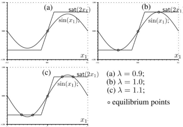
The equilibrium points of system (11) are given:
¯
x2= 0 and λsin ¯x1=sat(2¯x1)
where (¯x1,x¯2) represents the stationary solutions. Notice
that the number of equilibrium points will depend on the val-ues ofλ ∈ Bλ that lead to different possible solutions for
λsin ¯x1 −sat(2¯x1) = 0, see a graphical interpretation of
this equation in Figure 1.
−3.1 0.0 3.1
−1.50 0.00 1.50
−3.1 0.0 3.1
−1.50 0.00 1.50
−3.1 0.0 3.1
−1.50 0.00 1.50
−3.1 0.0 3.1
−1.50 0.00 1.50
−3.1 0.0 3.1
−1.50 0.00 1.50
−3.1 0.0 3.1
−1.50 0.00 1.50
x1
x1 x1
(a)λ= 0.9; (b)λ= 1.0; (c)λ= 1.1; sat(2x1)
sat(2x1) sat(2x1)
sin(x1); sin(x1);
sin(x1);
(a) (b)
(c)
equilibrium points
Figure 1: Equilibrium points equation: (a)λ= 0.9, (b)λ= 1and (c)λ= 1.1.
Also, the Jacobian matrix of system (11) is as follows:
A(¯x) =
"
0 1
λcosx1−∂
sat(2x1)
∂x1
−1
#
x=¯x (41)
where¯xrefers to the state vector evaluated at the equilibrium point.
Analyzing Figure 1 and taking into account (41), we have the following cases:
(a) λ= 0.9⇒one stable equilibrium point at system origin;
(b) λ = 1.0 ⇒ three equilibrium points at (0,0) (stable) and(±π/2,0)(non-hyperbolic points, see e.g. Seydel (1994));
(c) λ = 1.1 ⇒ five equilibrium points at(0,0),(±2.0,0)
(stables) and(±1.14,0)(unstables).
Clearly,(c)is the worst-case for estimating the stability re-gion in which the domain of attraction of(0,0)is bounded by two unstable equilibrium points at(1.14,0)and(−1.14,0). As these points are symmetrical with respect to the origin, both have the same Jacobian matrix which is given bellow:
A((±1.14,0)) =
0 1
0.46 −1
(42)
and associated with above matrix, we have the eigenvalues
σ1= 0.34,σ2=−1.34(characterizing a saddle point), and
the following eigenvectors:
υ1=
0.95
0.32
and υ2=
−0.60 0.80
. (43)
The above (real) eigenvectors have a geometrical meaning Seydel (1994). In fact, they define two straight lines passing through (±1.14,0) and each half-ray is a trajectory of the following linearized dynamics of (11) at(±1.14,0):
˙
z=A((±1.14,0))z
wherez=x−x¯. For the nonlinear problem, the eigenvector
υ2associated with the stable eigenvalueσ2 defines the
tan-gent to the incoming trajectories (stable manifold or insets) at(±1.14,0)and thus gives the approximate direction of the separatrix.
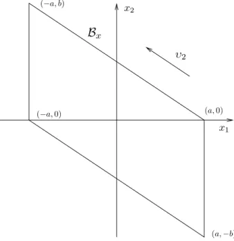
From the above analysis, we can construct the overbounding setBxby taking into account the unstable equilibrium points
(±1.14,0)and the eigenvectorυ2in (43) leading to the
poly-tope in Figure 2 (only represented inx1, x2sub-space) which
is defined by the following set of vertices:
a
−b c
,
a 0 c
,
−a
b c
,
−a
0 c
,
a
−b
−c
,
a 0
−c
,
−a
b
−c
,
−a
0
−c
(44)
wherea= 1.14,b= 2.67andc= sin(a).
In accordance with (44), define the admissible values ofτin (14) as follows:
Bτ =
h
x1
x2
υ
2B
x(a,0)
(a,−b) (−a,0)
(−a, b)
Figure 2: Overbounding polytopeBx.
+ + +
✁
✁
−1.20 −0.96 −0.72 −0.48 −0.24 0.00 0.24 0.48 0.72 0.96 1.20
−1.20 −0.96 −0.72 −0.48 −0.24 0.00 0.24 0.48 0.72 0.96 1.20
−1.20 −0.96 −0.72 −0.48 −0.24 0.00 0.24 0.48 0.72 0.96 1.20
−1.20 −0.96 −0.72 −0.48 −0.24 0.00 0.24 0.48 0.72 0.96 1.20
−1.20 0.00 1.20
−1.20 0.00 1.20
+ + + + + + + + + + + + + + + + + + + + + + + + + + + + + + +
−1.20 0.00 1.20
−1.20 0.00 1.20
+ + + + + + + + + + + + + + + + + + + + + + + + + + + + + + +
−1.20 0.00 1.20
−1.20 0.00 1.20
+++++++++++++++++++++++++++++++
−1.20 0.00 1.20
−1.20 0.00
1.20 +
+
+
+
+ +
+ +
+ +
+ ++
++++ ++++++++++++++
x1
x2
separatrix
R
pR
qFigure 3: Estimates of SR:Rq andRp.
For comparison purposes, we will consider to determine the stability region of system (11) the following partition for the matrixPin (15):
P =
P2 P1
P′
1 P0
, P2∈Rv×v, P0∈Rn×n
From above, we can obtain
i. Quadratic Lyapunov function: takeP0as a free matrix
and setP2= 0,P1= 0.
ii. Polynomial Lyapunov function: considerP0, P1andP2
as free matrices.
−3 −2 −1 0 1 2 3
−3 −2 −1 0 1 2 3
x1 x2
Figure 4: Phase portrait of system (11) .
Figure 3 shows estimates of the stability region of system (11) for an optimalρ = 2.0 whereRq was obtained with a quadratic Lyapunov function andRpwith a polynomial one. As expected, the polynomial Lyapunov function achieved the best estimate of SR thus justifying the required extra compu-tation.
Also, we give in Figure 4 the phase portrait of system (11) withλ = 1.1(the worst case for the real domain of attrac-tion). Notice that the SR of the origin is unbounded (and non-convex) and our method can only estimate closed sets (con-vex regions) which justifies the conservative result. How-ever, the proposed technique is potentially less conservative than the methods that consider quadratic Lyapunov functions (circle criterion) and can handle uncertainties on the system dynamics.
6
CONCLUDING REMARKS
How-ever, the authors are studying a systematic way of defining the differential-algebraic representation of nonlinear system and also the state domain (the region in which the stability conditions are analyzed) in order to turn the proposed ap-proach more appealing to the control community.
REFERENCES
Barreiro, A., Aracil, J. and Pagano, D. (2002). Detection of Attraction Domains of Nonlinear Systems Using the Bifurcation Analysis and Lyapunov Functions, Interna-tional Journal of Control75(5): 314–327.
Bean, S. P., Coutinho, D. F., Trofino, A. and Cury, J. E. R. (2002). Regional Stability of a Class of Nonlinear Hy-brid Systems: An LMI Approach, Proceedings of the 41th IEEE Conference on Decision and Control, Las Vegas.
Bender, D. J. and Laub, A. J. (1997). The Linear Quadratic Optimal Regulator for Descriptor Systems, IEEE Transactions on Automatic Control32(8): 672– 688.
Boyd, S., Ghaoui, L. E., Feron, E. and Balakrishnan, V. (1994). Linear matrix inequalities in systems and con-trol theory, SIAM books.
Chesi, G., Tesi, A. and Vicino, A. (2002). Computing Op-timal Quadratic Lyapunov Functions for Polynomial Nonlinear Systems via LMIs,Proceedings of the 15th IFAC World Congress, Barcelona, Spain.
Coutinho, D. F., Bazanella, A. S., Trofino, A. and Silva, A. S. (2002). Polynomial Lyapunov Functions for a Class of Differential-Algebraic Systems, Proceedings of the XIV Congresso Brasileiro de Automática, Natal, Brazil, pp. 110–115.
Coutinho, D. and Trofino, A. (2002). Análise de Sistemas Não Lineares Incertos: uma Abordagem LMI,Revista Controle e Automação13(2): 94–104.
Coutinho, D., Trofino, A. and Fu, M. (2002). Guaranteed Cost Control of Uncertain Nonlinear Systems via Poly-nomial Lyapunov Functions,IEEE Transactions on Au-tomatic Control47(9): 1575–1580.
Dussy, S. and El Ghaoui, L. (1997).Multi Objective Bounded Control of Uncertain Nonlinear Systems: An Inverted Pendulum Example, Lectures Notes in Control & Infor-mation Sciences, N. 227. Springer Verlag.
El Ghaoui, L. and Scorletti, G. (1996). Control of ratio-nal systems using linear-fractioratio-nal representations and LMIs,Automatica32(9): 1273–1284.
Finsler, P. (1937). Über das Vorkommen Definiter and Semidefiniter Formen in Scharen Quadratischer Form, Commentarii Mathematici Helvetici9: 188–192.
Gomes da Silva Jr., J. M. and Tarbouriech, S. (1999). In-variance and Contractivity of Polyhedra for Linear Countinuous-Time Systems with Saturating Controls, Revista Controle e Automação10(3): 149–156.
Hindi, H. and Boyd, S. (1998). Analysis of Linear Systems with Saturation using Convex Optimization, Proceed-ings of the 37th IEEE Conference on Decision and Con-trol, Tampa, pp. 903–908.
Huang, Y. and Jadbabaie, A. (1999). NonlinearH∞control:
an Enhanced Quasi-LPV Approach,Proceedings of the 14th IFAC World Congress, Beijing, China, pp. 85–90.
Huang, Y. and Lu, W.-M. (1996). Nonlinear Optimal Con-trol: Alternatives to Hamilton-Jacobi Equation, Pro-ceedings of the 35th IEEE Conference on Decision and Control, Kobe, Japan, pp. 3942–3947.
Johansen, T. A. (2000). Computation of Lyapunov Functions for Smooth Nonlinear Systems using Convex Optimiza-tion,Automatica36: 1617–1626.
Johansson, M. (2002). Piecewise Quadratic Estimates of Domain of Attraction for Linear Systems with Satu-ration,Proceedings of the 15th IFAC World Congress, Barcelona, Spain.
Kiyama, T. and Iwasaki, T. (2000). On the Use of Multi-loop Circle Criterion for Saturating Control Synthesis, System & Control Letters41: 105–114.
Seydel, R. (1994). Practical Bifurcation and Stability Anal-ysis: from equilibrium to chaos, Springer-Verlag.
Trofino, A. (2000). Robust Stability and Domain of Attrac-tion of Uncertain Nonlinear Systems, Proceedings of the American Control Conference, Chicago.