ISSN 0101-8205 www.scielo.br/cam
Mimetic finite difference methods in image processing
C. BAZAN1, M. ABOUALI1, J. CASTILLO1 and P. BLOMGREN2 1Computational Science Research Center, San Diego State University
5500 Campanile Drive, San Diego, CA 92182-1245, U.S.A.
2Department of Mathematics and Statistics, San Diego State University
5500 Campanile Drive, San Diego, CA 92182-7720, U.S.A. E-mails: [email protected] / [email protected] /
[email protected] / [email protected]
Abstract. We introduce the use of mimetic methods to the imaging community, for the solution of the initial-value problems ubiquitous in the machine vision and image processing and analysis fields. PDE-based image processing and analysis techniques comprise a host of ap-plications such as noise removal and restoration, deblurring and enhancement, segmentation, edge detection, inpainting, registration, motion analysis, etc. Because of their favorable stability and efficiency properties, semi-implicit finite difference and finite element schemes have been the methods of choice (in that order of preference). We propose a new approach for the numerical so-lution of these problems based on mimetic methods. The mimetic discretization scheme preserves the continuum properties of the mathematical operators often encountered in the image processing and analysis equations. This is the main contributing factor to the improved performance of the mimetic method approach, as compared to both of the aforementioned popular numerical solution techniques. To assess the performance of the proposed approach, we employ the Catté-Lions-Morel-Coll model to restore noisy images, by solving the PDE with the three numerical solution schemes. For all of the benchmark images employed in our experiments, and for every level of noise applied, we observe that the best image restored by using the mimetic method is closer to the noise-free image than the best images restored by the other two methods tested. These results motivate further studies of the application of the mimetic methods to other imaging problems.
Mathematical subject classification: Primary: 68U10; Secondary: 65L12.
Key words:mimetic methods, image processing, discrete operators, conservative methods.
1 Introduction
The aim of this paper is to introduce the mimetic methods to the imaging com-munity, for the solution of the initial-value problem ubiquitous in the machine vision and image processing and analysis fields. PDE-based image processing and analysis techniques comprise a host of applications such as noise removal and restoration, deblurring and enhancement, segmentation, edge detection, in-painting, registration, motion analysis, etc. In this context, a gray-scale image is
modeled as a real-valued functionu0(x),u0→R, defined in a bounded domain
⊂ R2, and with Lipschitz continuous boundary∂. Usually, the observed
imageu0(x)=u(x,0)is associated with a sequence of imagesu(x,t), where
the evolution depends on the abstract parametert >0, called the scale. Hence
the nameimage multiscale analysisgiven to this approach [30]. The numerical
solution of this problem is normally based on semi-discretization in scale and on finite difference or finite element discretization in space.
This paper is organized as follows: In Section 2, we briefly describe one of the most popular nonlinear diffusion models applied in image processing for the reduction of noise and the detection of edges. This serves as background for the readers who might not be familiar with PDE-based image processing techniques. In Section 3, we describe the mimetic discretization formulation for the solution of the initial-value problem. We also present the two most popular numerical solutions to this problem, namely finite difference and finite element methods. In Section 4, we present some computational examples of the performance of the proposed method as compared to the other two methods described in the previous section. We conclude the paper in Section 5 with a discussion of the reasons for the improved results obtained by applying the mimetic method. We also outline some possible future improvements to the this approach, and other areas within the imaging field where the method can be applied successfully.
2 Nonlinear diffusion models in image processing
nonlinear diffusion model aimed at avoiding the blurring of edges, and other localization problems presented by linear diffusion models [9, 26, 29, 44]. Their model accomplishes this by applying a process that reduces the diffusivity in places having higher likelihood of belonging to edges. This likelihood is
meas-ured by a function of the local gradient,|∇u|. The Perona-Malik model can be
written as
ut − ∇ ∙ g |∇u|2
∙ ∇u
=0, on ×[0,∞) ,
u(x,0)=u0(x) , on ,
hg∙ ∇u,ni =0, on ∂×(0,∞) ,
(1)
wherehg∙ ∇u,ni =0 denotes homogeneous Neumann boundary conditions. In
this model the diffusivity has to be such thatg |∇u|2
→0 when|∇u| → ∞
andg |∇u|2 → 1 when|∇u| → 0. One of the diffusivities that Perona and
Malik proposed isg |∇u|2= 1+ |∇u|2λ2−1, whereλ > 0 is a threshold
(contrast) parameter that separates forward and backward diffusion [38]. The model accomplishes the long sought effect of blurring small fluctuations (pos-sible noise) while enhancing edges. The results obtained by Perona and Malik were visually very impressive.
Notwithstanding the practical success of the Perona-Malik model, it presents some serious theoretical problems: (i) none of the classical well-posedness
frameworks is applicable to the Perona-Malik model, i.e. we can not ensure
well-posedness results [34, 42]; (ii) uniqueness and stability with respect to the
initial image should not be expected,i.e. solvability is a difficult problem, in
general [15, 21, 22, 25, 36]; (iii) the regularizing effect of the discretization plays too much of an important role in the solution [6, 17]. The latter is perhaps the key element in the success or failure of the model. Most practical applica-tions work very well provided that the numerical schemes stabilize the process through some implicit (or explicit) regularization.
This observation motivated much research towards the introduction of the regularization directly into the PDE to avoid the dependence on the numerical schemes [15, 34]. A variety of spatial, spatio-temporal, and temporal regular-ization procedures have been proposed over the years [5, 15, 28, 38, 40, 43]. The one that has attracted much attention is the mathematically sound formu-lation due to Catté, Lions, Morel and Coll [15]. They proposed replacing the
diffusivityg |∇u|2
of the Perona-Malik model by a slight variationg |∇uσ|2
withuσ = Gσ ∗u, where Gσ is a smooth kernel (Gaussian of variance σ2).
We should note that this spatial regularization model belongs to a class of well-posed problems (existence and uniqueness were proven in [15]), and that its successful implementation is contingent on the choosing of an appropriate value
for the additional regularization parameterσ. Whitaker and Pizer [43] and Li
and Chen [28] suggested making the parametersσ andλtime-dependent, while
Benhamouda [6] performed a systematic study of the influence of these param-eters for the one-dimensional case.
3 Numerical solution to the nonlinear diffusion models
Digital images are given on discrete (regular) grids. This lends itself for dis-cretizing the PDEs to obtain numerical schemes that can be solved on a com-puter. Because of their favorable stability and efficiency properties, semi-im-plicit schemes have been the methods of choice for the scale discretization [3, 4, 15, 16, 18, 19, 20, 24, 27, 31, 32, 37, 39, 41]. As for the space dis-cretization, the most popular choices are finite difference [15, 39, 41] and finite element [3, 4, 16, 24, 37, 39, 41] methods (in that order of preference). We propose a new approach in image processing based on mimetic discretization.
3.1 Finite difference implementation
The numerical solution to the Catté-Lions-Morel-Coll model proposed in [15]
is as follows. Given an N × M image we introduce the coordinates lattice
(i h, j h,n1t)whereh is the pixel size, and 0 6i 6 N +1, 06 j 6M+1. We consideruni,j as an approximation ofu(i h, j h,n1t), andgi,jn as an approx-imation of g(|∇uσ|) (i h,j h,n1t). Then we discretise g(|∇uσ|) ∂u
∂x by
gn i,j∂u
∂x(i h, j h, (n+1) 1t)and∂∂x
g(|∇uσ|) ∂u
∂x by
gi−n 1,j +gi,njun+i−11,j−2gi,nj+gni−1,j +gi+n 1,jui,n+j1+gi,jn +gin+1,jun+i+11,j
2h2 ,
and similarly for∂
∂y
g(|∇uσ|) ∂u
∂y
, by exchanging the roles of parame-tersiand j,
gi,jn −1+gi,jn ui,jn+−11−2gni,j+gni,j−1+gni,j+1un+i,j1+gi,jn +gi,jn +1un+i,j+11
The finite difference scheme will be given by
un+i,j1−uni,j
1t −
1 2h2
h
gni−1,j +gi,njun+i−11,j + gni,j−1+gi,njun+i,j−11+ + gni,j +gin+1,jun+i+11,j+ gni,j +gi,nj+1un+i,j+11+
− 4gi,jn +gni−1,j +gni,j−1+gi+n 1,j +gi,nj+1un+i,j1
i
=0,
u0i,j =u0(i h, j h) , 16i 6N, 16 j 6M,
ui,n+01=ui,n+11, un+N,1j =un+N+11,j, 16i 6 N+1, 16 j6 M+1, u0n+,j1=u1n+,j1, un+i,N1=ui,N+n+11, 16i6 N+1, 16 j 6M+1.
(2)
Then, the discrete problem can be written as a system
un+1−un
1t +Ah u
n
un+1=0, n >0, (3)
where the matrix of coefficientsAhis positive definite and block-tridiagonal.
3.2 Finite element implementation
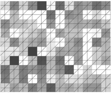
The starting point for the finite element method is to partition the geometry (domain) into small units (elements or cells) of simple shape joined together at the vertices (nodes). This will constitute our finite element space (mesh or grid). Once we have our mesh (see Fig. 1), the idea is to approximate the dependent variables with functions that we can describe with a finite number of parameters (degrees of freedom, DOF). Inserting this approximation into the weak form of the equation for the Catté-Lions-Morel-Coll model generates a system of equations for the degrees of freedom [1].
As mentioned above, we need to perform discretizations in scale and space.
We perform the semi-discretization in scale by lettingQ ∈ N, and1t = TQ
be fixed numbers (here,T represents the last scale state we want to reach), and
lettingu(x,0) = u0(x) in. Then, we can look for a functionun for every
n=1, . . . ,Q, such that it is a solution to the equation
un−un−1 1t − ∇ ∙
g
∇un−σ 1
2
∙ ∇un
Figure 1 – Zoomed-in detail of an image at the pixel level. The image was superimposed
with a finite element mesh of triangular elements. Each node of an element has one DOF, the intensity value of that pixel.
It is shown in [4, 24] that there exist unique variational solutionsun of Eq. (4)
at every discrete scale step, for which the following stability estimates hold:
un
26ku0k2,
un
∞6ku0k∞, forn =1, . . . ,Qon Q
X
n=1
∇un
2
2h 6C,
Q
X
n=1
un−un−1
2
26C, on ,
(5)
whereC is a general (large) constant (here,hrepresents a typical element size).
To discretize the problem in space we can take advantage of the pixel structure of the image. For this case, the finite element method assumes that the approxima-tion of the soluapproxima-tion to the PDE is continuous piecewise linear. This means that the discrete intensity values are regarded as approximations of the continuous intensity function in the center of the pixels (see Fig. 1). We can multiply Eq. (4)
by an arbitrary test functionv ∈ V, whereV is the Sobolev spaceW1,2()of
L2()−functions with doubly integrable weak derivatives, and integrate (using
Green’s theorem and homogeneous Neumann boundary conditions) to obtain the weak form [30]
Z
unvd x+1t
Z
g
∇un−σ 1
2
∇un∇vd x =
Z
Then, for each scale stepn, we look for a continuous piecewise linear function
un
h∈ Vhthat satisfies
Z
unhvhd x+1t
Z
g∇un−h 1
2
∇unh∇vhd x =
Z
un−h 1vhd x, (7)
for allvh ∈ Vh. Considering the standard Lagrangian base functions φq ∈ Vh,
q = 1, . . . ,L, given by φq xp
= δq p (Kronecker delta) for all nodes, the
functionunhis given by
unh=
L
X
p=1
unpφp. (8)
Substituting Eq. (8) into Eq. (7) and considering as test functionsvh = φq for
q =1, . . . ,L, we get the Ritz-Galerkin equation for the nodal valuesunp, of the piecewise linear functionunh:
L
X
p=1
Z
φpφqd x +1t
Z
g
∇unσ,h
2
∇φp∇φqd x
unp=
=
Z
unhφqd x, q =1, . . . ,L.
(9)
Then, in each scale step we need to assemble and solve a linear system of the form
h
M+1tA
g∇un−σ 1
2i
un =fn−1, (10)
for the vector of unknowns (DOF)un.
3.3 Mimetic discretization implementation
exact.” For this reason, the mimetic discretization method has shown to be more stable and accurate than other numerical discretization methods [11, 12, 8, 23]. Here, we present only the second-order accuracy mimetic gradient and diver-gence operators developed by Castillo and Grone [10, 14] that were used in our numerical experiments. For a detailed explanation of how these operators were developed we refer the reader to [10, 14] and the references therein.
The Catté-Lions-Morel-Coll variant to Eq. (1) can be written using mimetic operators as
ut −D g |Guσ|2
Gu=0, (11)
whereDis the mimetic divergence operator,∇∙, andGis the mimetic gradient
operator, ∇. In one dimension and on a uniform staggered grid, the mimetic
gradient operator with second order accuracy is defined as
G= 1 h −8 3 3 −1 3
−1 1
−1 1
∙ ∙ ∙ −1 1
−1 1 8
3 −3
1 3 , (12)
wherehis the grid spacing. Likewise, the mimetic divergence is defined as
D= 1 h
−1 1
−1 1
∙ ∙ ∙
−1 1
−1 1 . (13)
The divergence matrix Dsatisfies some desired properties listed in [10]. These
properties are:
• Dhas zero row sums, i.e., De=0, where e=(1,1, . . . ,1)T. • Dhas column sums−1,0, . . . ,0,1, i.e., eTD=(−1,0,0, . . . ,0,1).
• Dhas a Toeplitz-type structure on the interior rows and is defined inde-pendently of the number of grid points.
One of the mimetic method’s interesting properties is that the matrix D and
Gare centro-skew-symmetric. It has to be noted that the gradient and the
diver-gence are not calculated at the same position. The gradient is calculated at the edges of the cell, whereas the divergence is calculated at the center of the cell (see Fig. 2).
Figure 2 – Positions where the one dimensional Gradient (G) and Divergence (D) are
calculated.
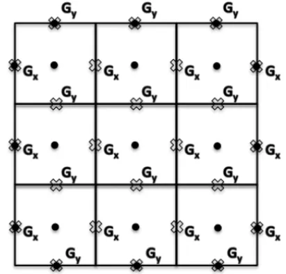
In two dimensions, the positions where the gradient is calculated is shown
in Fig. 3. Notice that the x-component and y-component of the gradient are
calculated separately and in different positions. This is important when design-ing a parallel code. Similarly, the position where the divergence is calculated is shown in Fig. 4. Notice that the mimetic gradient and mimetic divergence are designed in such way that the output of the mimetic gradient is positioned exactly where the mimetic divergence reads its input.
One of the advantages of the mimetic gradient and mimetic divergence de-veloped by Castillo and Grone is the way in which they represent the boundary conditions. The Neumann boundary conditions imposed in Eq. (1) dictate that the flux through the boundaries is zero. This is equivalent to saying that the normal component of the gradient to the boundary is zero. By referring to Fig. 3, we can understand that, to impose this boundary condition, all we have to do is set the gradient at the boundary to be zero. This has a great advantage. Usually the boundary conditions and their implementation is a major source of errors in numerical modeling and simulation. To implement the boundary conditions, normally some type of interpolation, extrapolation, or the use of ghost/dummy nodes is needed. Here, in this article, the boundary conditions dictate that the normal component of the gradient at the edges of the image must be zero, Eq. (1). To calculate the normal component of the gradient at the outer edges of
the image using the mimetic method, we need the value ofuat the center of the
two cells adjacent to the edge and also its value on the edge itself, see Fig. 3 and
Figure 3 – Two dimensional mimetic gradient operator. (circle) Positions whose values
are used to calculate the gradient. (cross) Positions where the gradient is calculated.
Figure 4 – Two dimensional mimetic divergence operator. (circle) Positions whose values are used to calculate the divergence. (cross) Positions where the divergence is
calculated.
ofujust at the cell centers and not the outer edges. To get the value ofuat the
outer edges we have to use the extrapolation techniques. The value ofu at the
and for the same component that our mimetic method calculates the gradient. Hence, there is no need for any extrapolation or use of dummy nodes to imple-ment the boundary conditions. Therefore, using Castillo Grone mimetic method, one big source of error can be eliminated.
4 Numerical experiments and results
In order to compare the performance of the mimetic discretization we imple-mented the Perona-Malik variant by Catté, Lions, Morel and Coll,
ut− ∇ ∙ g |∇uσ|2
∙ ∇u
=0, on ×[ 0,∞) ,
u(x,0)=u0(x) , on ,
hg∙ ∇u,ni =0, on ∂×(0,∞) ,
g |∇uσ|2
= 1
1+ |∇uσ|2
λ2, λ >0,
uσ =Gσ ∗u, σ =1.
(14)
It has been shown [33] that σ = 1 is sufficient for a large interval of noise
variances, provided that the noise in neighboring pixels is uncorrelated and that
the grid size is one. There are several ways to set the parameterλ > 0. Perona
and Malik [35] suggested using the idea presented by Canny [9] and setλ as
a percentile, p, of the image gradient magnitudes at each iteration. (The
rec-ommended value is commonly p = 90%.) A by-product of this approach is a
decreasingλ, which has an stabilizing effect on the diffusion process [33]. A
time step ofδt=10−2was chosen to update all the models. Weickert, Romeny,
and Viergever [41] have shown that, for explicit discretization schemes, the
sta-bility condition, assumingδx = 1 and∀s :g(s) 6 1, isδt < 1(2d), withd
being the number of dimensions of the data (which for a 2D imaged =2).
The experiment consisted in trying to restore the noise-free image f (x),
that has been perturbed by additive Gaussian noise of zero mean and variance
0.001>ν >0.02. Figure 1 shows the images of the Cameraman, the Baboon,
image to the noise-free image after restoration. For every benchmark image and for every level of noise, we observe that the best image restored by the mimetic discretization is closer to the noise-free image than the best images restored by the other two methods tested (see Figs. 2, 4, 6, and 8). The quality of the image restoration after applying the three solution methods to the noisy benchmark images is illustrated in Figs. 3, 5, 7, and 9.
Figure 5 – Noise-free images of the Cameraman, the Baboon, the Boats, and Barbara. These are the benchmark images that will be used in the comparative experiments.
5 Conclusion
In this paper we introduced the mimetic discretization method for the numer-ical solution of the PDE-based image processing and analysis models. The mimetic discretization scheme preserves the continuum properties of the math-ematical operators often encountered in the image processing and analysis equa-tions. This contributes to the stability and accuracy of the numerical solution which allows for the improved performance of the approach, as compared to the two very popular numerical solution techniques employed in our experiments. In these experiments, we applied a wide range of noise levels to benchmark images commonly used in the imaging field. These images were restored by applying the well stablished Catté-Lions-Morel-Coll model. Our results show that, for each noise level, the best image that has been restored by solving the PDE with the mimetic discretization scheme, outperforms the best images that have been restored by solving the PDE with the other two methods.
0.004 0.008 0.012 0.016 0.02 0.96
0.97 0.98 0.99 1.00
Variance of the Noise
Q
u
a
lit
y
o
f
R
e
st
o
ra
ti
o
n
Benchmark Image Cameraman FD MD FE
5 10 15 20 25 30 35 40 45 50 0.93
0.94 0.95 0.96 0.97 0.98
Number of Iterations
Q
u
a
lit
y
o
f
R
e
st
o
ra
ti
o
n
Restoration Comparison Cameraman FD MD FE
Figure 6 – (Left) Correlation coefficient between the noise-free image of the
Camera-man and the filtered image of the CameraCamera-man. For every noise level, the best filtered image restored by using the mimetic discretization is superior to the best filtered
im-ages restored by using the finite difference and the finite element methods, respec-tively. (Right) Typical path of the quality of the image restoration. For a noise variance
ν =0.01, the quality of restoration increases to a maximum value after which it
de-creases asymptotically as the image becomes ‘flat.’ The best filtered image for this level
of noise is obtained after 17 iterations by finite difference, 4 iterations by finite element,
and 6 iterations by mimetic discretization.
Figure 7 – (Left to Right) Noisy image of the Cameraman perturbed by Gaussian
ad-ditive noise of zero mean and varianceν =0.01. Filtered image of the Cameraman
after 17 iterations by the finite difference method. Filtered image of the Cameraman after 4 iterations by the finite element method. Filtered image of the Cameraman after
0.004 0.008 0.012 0.016 0.02 0.84 0.86 0.88 0.90 0.92 0.94 0.96 0.98 1.00
Variance of the Noise
Q u a lit y o f R e st o ra ti o n
Benchmark Image Baboon FD MD FE
5 10 15 20 25 30 35 40 45 50 0.84 0.85 0.86 0.87 0.88 0.89 0.90 0.91 0.92
Number of Iterations
Q u a lit y o f R e st o ra ti o n
Restoration Comparison Baboon FD MD FE
Figure 8 – (Left) Correlation coefficient between the noise-free image of the Baboon and the filtered image of the Baboon. For every noise level, the best filtered image
restored by using the mimetic discretization is superior to the best filtered images
re-stored by using the finite difference and the finite element methods, respectively. (Right) Typical path of the quality of the image restoration. For a noise varianceν=0.01, the
quality of restoration increases to a maximum value after which it decreases asymp-totically as the image becomes ‘flat.’ The best filtered image for this level of noise is
obtained after 10 iterations by finite difference, 3 iterations by finite element, and 4 iterations by mimetic discretization.
Figure 9 – (Left to Right) Noisy image of the Baboon perturbed by Gaussian
addit-ive noise of zero mean and varianceν = 0.01. Filtered image of the Baboon after 10 iterations by the finite difference method. Filtered image of the Baboon after 3
0.004 0.008 0.012 0.016 0.02 0.92 0.93 0.94 0.95 0.96 0.97 0.98 0.99 1.00
Variance of the Noise
Q u a lit y o f R e st o ra ti o n
Benchmark Image Boats
FD MD FE
5 10 15 20 25 30 35 40 45 50 0.88 0.89 0.90 0.91 0.92 0.93 0.94 0.95 0.96 0.97
Number of Iterations
Q u a lit y o f R e st o ra ti o n
Restoration Comparison Boats FD MD FE
Figure 10 – (Left) Correlation coefficient between the noise-free image of the Boats and the filtered image of the Boats. For every noise level, the best filtered image
stored by using the mimetic discretization is superior to the best filtered images re-stored by using the finite difference and the finite element methods, respectively. (Right)
Typical path of the quality of the image restoration. For a noise varianceν=0.01, the
quality of restoration increases to a maximum value after which it decreases asymp-totically as the image becomes ‘flat.’ The best filtered image for this level of noise is
obtained after 17 iterations by finite difference, 5 iterations by finite element, and 7 iterations by mimetic discretization.
Figure 11 – (Left to Right) Noisy image of the Boats perturbed by Gaussian additive noise of zero mean and varianceν =0.01. Filtered image of the Boats after 17
itera-tions by the finite difference method. Filtered image of the Boats after 5 iteraitera-tions by
0.004 0.008 0.012 0.016 0.02 0.93 0.94 0.95 0.96 0.97 0.98 0.99 1.00
Variance of the Noise
Q u a lit y o f R e st o ra ti o n
Benchmark Image Barbara FD MD FE
5 10 15 20 25 30 35 40 45 50 0.86 0.88 0.90 0.92 0.94 0.96 0.98
Number of Iterations
Q u a lit y o f R e st o ra ti o n
Benchmark Image Barbara
FDM MDM FEM
Figure 12 – (Left) Correlation coefficient between the noise-free image of Barbara and the filtered image of Barbara. For every noise level, the best filtered image restored
by using the mimetic discretization is superior to the best filtered images restored by using the finite difference and the finite element methods, respectively. (Right) Typical
path of the quality of the image restoration. For a noise varianceν =0.01, the quality of restoration increases to a maximum value after which it decreases asymptotically
as the image becomes ‘flat.’ The best filtered image for this level of noise is obtained
after 24 iterations by finite difference, 9 iterations by finite element, and 10 iterations by mimetic discretization.
Figure 13 – (Left to Right) Noisy image of Barbara perturbed by Gaussian additive
noise of zero mean and varianceν = 0.01. Filtered image of Barbara after 24
itera-tions by the finite difference method. Filtered image of Barbara after 9 iteraitera-tions by the finite element method. Filtered image of Barbara after 10 iterations by the
REFERENCES
[1] COMSOL AB, COMSOL Multiphysics Modeling Guide v3.2. COMSOL AB, Burlington, Massachusetts (2005).
[2] B. Aulbach and S. Hilger, Linear dynamic processes with inhomogeneous time scale. Nonlinear Dynamics and Quantum Dynamical Systems (1990).
[3] E. Bänsch and K. Mikula, A coarsening finite element strategy in image selective smoothing.Computing and Visualization in Science,1(1) (1997), 53–61. [4] E. Bänsch and K. Mikula, Adaptivity in 3D image processing. Computing and
Visualization in Science,4(1) (2001), 21–30.
[5] G.I. Barenblatt, M. Bertsch, R. Dal Passo and M. Ughi, A degenerate pseudo-parabolic regularization of a nonlinear forward-backward heat equation arising in the theory of heat and mass exchange in stably stratified turbulent shear flow.
SIAM Journal on Mathematical Analysis,24(6) (1993), 1414–1439.
[6] B. Benhamouda, Parameter adaptation for nonlinear diffusion in image pro-cessing. Master’s thesis, University of Kaiserslautern, Kaiserslautern, Germany (1994).
[7] P.B. Bochev and J.M. Hyman,Principles of mimetic discretizations of differential operators. The IMA Volumes in Mathematics and its Applications,142(2006), 89–119.
[8] M. Bohner and J.E. Castillo, Mimetic methods on measure chains. Computers and Mathematics with Applications,42(2001), 705–710.
[9] A. Canny, A computational approach to edge detection. IEEE Transactions on Pattern Analysis and Machine Intelligence,8(6) (1986), 679–698.
[10] J.E. Castillo and R.D. Grone, A matrix analysis approach to higher-order ap-proximations for divergence and gradients satisfying a global conservation law.
SIAM Journal on Matrix Analysis and Applications,25(1) (2003), 128–142.
[11] J.E. Castillo and J.M. Hyman, Fourth and sixth-order conservative finite differ-ence approximations of the divergdiffer-ence and gradient. Applied Numerical Math-ematics,37(1-2) (2001), 171–187.
[12] J.E. Castillo, J.M. Hyman, M.J. Shashkov and S. Steinberg, The sensitivity and accuracy of forth order finite-difference schemes on nonuniform grids in one di-mension.Computers and Mathematics with Applications,30(8) (1995), 41–55.
[14] J.E. Castillo and M. Yasuda, Linear systems arising for second-order mimetic divergence and gradient discretizations. Journal of Mathematical Modeling and Algorithms,4(2005), 67–82.
[15] F. Catté, P.-L. Lions, J.-M. Morel and T. Coll, Image selective smoothing and edge detection by nonlinear diffusion. SIAM Journal of Numerical Analysis, 29(1) (1992), 182–193.
[16] U. Diewald, T. Preusser, M. Rumpf and R. Strzodka, Diffusion models and their accelerated solution in image and surface processing. Acta Mathematica Univer-sitatis Comenianae,70(1) (2001), 15–34.
[17] J. Fröhlich and J. Weickert, Image processing using a wavelet algorithm for nonlinear diffusion. Report 104, Laboratory of Technomathematics, University of Kaiserslautern, Kaiserslautern, Germany (1994).
[18] A. Handlovi˘cová, K. Mikula and A. Sarti,Numerical solution of parabolic equa-tions related to level set formulation of mean curvature flow. Computing and visualization in Science,1(2) (1999), 179–182.
[19] A. Handlovi˘cová, K. Mikula and F. Sgallari, Variational numerical methods for solving nonlinear diffusion equations arising in image processing. Journal for Visual Communication and Image Representation,13(1-2) (2002), 217–237.
[20] A. Handlovi˘cová, K. Mikula and F. Sgallari, Semi-implicit complementary vol-ume scheme for solving level set like equations in image processing and curve evolution. Numerische Mathematik,93(4) (2003), 675–669.
[21] K. Höllig, Existence of infinitely many solutions for a forward-backward heat equation. Transactions of the American Mathematical Society, 278(1) (1983), 299–319.
[22] K. Höllig and J.A. Nohel,A diffusion equation with a non-monotone constitutive function.In: J.M. Ball (ed.), Proceedings of NATO/London Mathematical Society Conference on Systems of Partial Differential Equation, pages 409–422, (1983).
[23] J.M. Hyman and S. Steinberg, The convergence of mimetic discretization for rough grids. Computers and Mathematics with Applications,47(10-11) (2004), 1565–1610.
[24] J. Ka˘cur and K. Mikula, Solution of nonlinear diffusion appearing in image smoothing and edge detection. Applied Numerical Mathematics, 17(1) (1995), 47–59.
[25] S. Kichenassamy, The Perona-Malik paradox. SIAM Journal of Applied Math-ematics,57(5) (1997), 1328–1342.
[27] Z. Krivá and K. Mikula, An adaptive finite volume scheme for solving nonlinear diffusion in image processing. Journal for Visual Communication and Image Representation,13(1-2) (2002), 22–35.
[28] X. Li and T. Chen,Nonlinear diffusion with multiple edginess thresholds.Pattern Recognition,27(8) (1994), 1029–1037.
[29] D. Marr and E. Hildreth, Theory of edge detection. In: Proceedings of Royal Society of London. Series B, Biological Sciences, Royal Society Publishing, 207(1980), 187–217.
[30] K. Mikula, Image processing with partial differential equations, volume 75 of Modern Methods in Scientific Computing and Applications, NATO Science Series II, pages 283–322. Kluwer Academic Publishers, Dodrecht, Netherlands (2002).
[31] K. Mikula and N. Ramarosy,Semi-implicit finite volume schemes for solving non-linear diffusion equations in image processing.Numerische Mathematik, 89(3) (2001), 561–590.
[32] K. Mikula, A. Sarti and C. Lamberti, Geometrical diffusion in 3-d-echocardio-graphy. In: J. Ka˘cur and K. Mikula (eds.), Proceedings of ALGORITMY ’97, Conference on Scientific Computing, volume 67, pages 167–181. Acta Mathem-atica Universitatis Comenianae (1998).
[33] P. Mrázek, Nonlinear Diffusion for Image Filtering and Monotonicity Enhance-ment. PhD thesis, Czech Technical University, Prague, Czech Republic (2001).
[34] M. Nitzberg and T. Shiota, Nonlinear image filtering with edge and corner en-hancement. IEEE Transactions on Pattern Analysis and Machine Intelligence, 14(8) (1992), 826–833.
[35] P. Perona and J. Malik,Scale space and edge detection using anisotropic diffusion.
IEEE Transactions on Pattern Analysis and Machine Intelligence, 12(7) (1990), 629–639.
[36] P. Perona, T. Shiota and J. Malik,Anisotropic diffusion. In: B.M. ter Haar Romeny (ed.), Geometry-Driven Diffusion in Computer Vision, volume 1 of Computational Imaging and Vision, pages 72–92. Springer, Kluwer (1994).
[37] T. Preusser and M. Rumpf, An adaptive finite element method for large scale image processing. In Proceedings of Scale-Space ’99, pages 223–234, (1999). [38] J. Weickert, Anisotropic Diffusion in Image Processing. PhD thesis, Universität
Kaiserslautern, Kaiserslautern, Germany (1996).
[40] J. Weickert, Efficient image segmentation using partial differential equations and morphology.Pattern Recognition,34(9) (2001), 1813–1824.
[41] J. Weickert, B.M.t.H. Romeny and M.A. Viergever, Efficient and reliable schemes for nonlinear diffusion filtering. IEEE Transactions on Image Process-ing,7(3) (1998), 398–410.
[42] J. Weickert and C. Schnörr,PDE-based preprocessing of medical images. Kunst-liche Intelligenz,3(2000), 5–10.
[43] R.T. Whitaker and S.M. Pizer, A multi-scale approach to non-uniform diffu-sion. Computer Vision, Graphics, and Image Processing: Image Understanding, 57(1) (1993), 99–110.