Análise de estabilidade de sistemas de potência em presença de altos níveis de penetração...

(1)

DAVID JOEL FIGUEROA CORTÉS

Analysis of power system stability in presence of high levels of

wind power penetration

(2)

DAVID JOEL FIGUEROA CORTÉS

Analysis of power system stability in presence of high levels of

wind power penetration

Dissertação

apresentada

à

Escola

Politécnica da Universidade de São Paulo

para obtenção do título de Mestre em

Ciências

Orientador: Prof.

Mauricio Barbosa de Camargo Salles.

(3)

DAVID JOEL FIGUEROA CORTÉS

Analysis of power system stability in presence of high levels of

wind power penetration

Dissertação

apresentada

à

Escola

Politécnica da Universidade de São Paulo

para obtenção do título de Mestre em

Ciências

Área de Concentração:

Engenharia Elétrica

Orientador: Prof.

Mauricio Barbosa de Camargo Salles.

(4)

Este exemplar foi revisado e corrigido em relação à versão original, sob

responsabilidade única do autor e com a anuência de seu orientador.

São Paulo, 12 de agosto de 2014.

Assinatura do autor ____________________________

Assinatura do orientador _______________________

Catalogação-na-publicação

I.

II.

III.

IV.

V.

VI.

VII.

VIII. Catalogação-na-publicação

Figueroa Cortes, David Joel

Analysis of power system stability in presence of high

levels of wind power penetration / D.J. Figueroa Cortes. -- versão corr. -- São Paulo, 2014.

130 p.

Dissertação (Mestrado) - Escola Politécnica da Universidade de São Paulo. Departamento de Engenharia de Energia e Auto-mação Elétricas.

(5)

I dedicate this work to these people whose encouragement and support were really important

in the development and the achievement of the same, maybe without them, none of this would

have been successfully completed:

(6)

ACKNOWLEDGEMENTS



To the professor Mauricio Salles, for the support and orientation during the

development of this work;



To the professors of the Laboratório de Elegtromagnetismo Aplicado (LMAG) for the

support;



To the colleagues with whom I shared in the LMAG during the development of this

masters degree;



To my friends from the Escola Politécnica of the Universidade de São Paulo (USP);



To the Coordenação de Aperfeiçoamento de Pessoal de Nível Superior (CAPES) and

the Fundação de Apoio à Universidade de São Paulo (FUSP) for the financial support;



To my family and friends for the emotional support and encouragement;

(7)

RESUMO

Atual

ment

e, a energia eólica é uma das fontes renováveis mais reconhecidas, e sua

penetração em sistemas elétricos de potência está se incrementando consideravelmente. Por

consequência, a participação de turbinas eólicas em sistemas elétricos de potência tem se

incrementado e pode influenciar o comportamento geral do sistema de potência. Portanto,

é

importante estudar o desempenho de turbinas eólicas em sistemas elétricos e sua interação

com outros equipamentos de geração e cargas. O principal objetivo nesta dissertação é

determinar o desempenho dinâmico de diferentes tecnologias ligadas nos sistemas elétricos

considerando diferentes níveis de penetração e diferentes perturbações elétricas mediante

simulações realizadas usando um

toolbox

de Matlab/Simulink, SimPowerSystems. As

tecnologias avaliadas são (a) o gerador de indução duplamente alimentado com fator de

potência unitário, (b) o gerador de indução duplamente alimentado com controle de tensão, (c)

o gerador de indução de gaiola de esquilo com compensação baseada em condensadores, e (d)

gerador de indução de gaiola de esquilo sem equipamentos auxiliares. Os fatores técnicos

analisados são perfil de tensão em estado estacionário, as dinâmicas durante afundamentos e

elevações de tensão, correntes de curto circuito, e incremento gradual nas cargas do sistema,

para verificar a estabilidade de tensão da rede para pequenas perturbações. É proposta uma

estratégia para promover uma integração efetiva de turbinas eólicas em sistemas de potência

com altos níveis de penetração considerando diferentes normas de operação da rede para

sistemas de transmissão e de distribuição. O objetivo nesta estratégia é o cumprimento dos

requisitos para conexão de rede com a combinação de tecnologias, minimizando o valor do

investimento. Os efeitos na estabilidade de sistemas de potência da fazenda eólica

determinada com a metodologia proposta são comparados com os efeitos de uma fazenda

eólica de igual capacidade de energia eólica considerando somente geradores de indução

duplamente alimentados com controle de tensão. Para as analises realizadas neste trabalho são

considerados os sistemas IEEE de 9 e 30 barras.

(8)

ABSTRACT

Nowadays, wind power is one of the most accepted renewable energy sources, and its

penetration in electrical power systems is increasing considerably. Consequently, the

participation of wind turbines in electrical power systems has increased and may influence the

overall power system behavior. It is therefore important to study the performance of wind

turbines in electrical power systems and their interaction with other generation equipment and

loads. The main objective of this dissertation is to determine the dynamic performance of

different wind turbines technologies connected in electrical system considering different

penetration levels and electrical perturbations by simulations performed using a

Matlab/Simulink toolbox, SimPowerSystems. The assessed technologies are (a) double fed

induction generator with unity power factor, (b) double fed induction generator with voltage

control, (c) squirrel cage induction generator with capacitor-based compensation, and (d)

squirrel cage induction generator without ancillary devices. The technical factors analyzed are

steady-state voltage profile, the dynamics during voltage sags and swells, short-circuit

currents, and gradual increase in the system loading, in order to check the network

small-disturbance voltage stability. A strategy to promote an effective integration of wind turbines

into the power systems with high levels of wind power penetration regarding different grid

code requirements in transmission and distribution networks is proposed. The objective in this

strategy is fulfilling the grid code requirements with a technology combination, minimizing

the invested value. The effects on power system stability of the wind farm, found by the

proposed methodology, are compared with the effects that have the same installed capacity of

wind power but only considering double fed induction generators with voltage control. The

IEEE 9 bus transmission system and the IEEE 30 bus system are regarded for the analysis

performed in this work.

(9)

LIST OF FIGURES

Figure 2.1 – Top 10 cumulative capacities (December 2012)... 23

Figure 2.2 – Top 5 in offshore wind [MW]. ... 23

Figure 2.3 – Continental shares in total capacity [%]. ... 24

Figure 2.4 – Timeline of wind power evolution. ... 24

Figure 2.5 – World total installed capacity [GW]. ... 25

Figure 2.6 – Brazilian wind power capacity [MW]. ... 27

Figure 2.7 – Danish wind power capacity and its share of domestic electricity supply. ... 28

Figure 2.8 – German wind power capacity and its share of domestic electricity supply. ... 29

Figure 2.9 – Irish wind power capacity and its share of domestic electricity supply. ... 30

Figure 2.10 – Japanese wind power capacity [MW]. ... 31

Figure 2.11 – Portuguese wind power capacity and its share of domestic electricity supply. ... 31

Figure 2.12 – Spanish wind power capacity and its share of domestic electricity supply. ... 32

Figure 2.13 – Installed wind power capacity forecasts. ... 33

Figure 3.1 – Wye connected load for static analysis. ... 35

Figure 3.2 – Wye connected load for dynamic analysis. ... 36

Figure 3.3 – Transmission line π model. ... 37

Figure 3.4 – Equivalent circuit for a single-phase transformer with an ideal transformer of turns ratio . ... 37

Figure 3.5 – Equivalent circuit for a single-phase generator or synchronous condenser. ... 38

Figure 3.6 – Equivalent circuit of synchronous generator. ... 39

(10)

Figure 3.8 – Equivalent circuit of the induction machine. ... 40

Figure 3.9 – DFIG wind power system topology. ... 42

Figure 3.10 – 69 Bus system considering 16 generators. ... 44

Figure 3.11 – Reactive power for three-phase fault at middle of one of lines 60–61 (solid line synchronous generator and dashed line DFIG). ... 45

Figure 3.12 – Voltage at bus 49 for three-phase fault at middle of one of lines 60–61 (solid line synchronous generator, and dashed line 60% DFIGs and 40% SGs)... 46

Figure 3.13 – WSCC 3-gen-9-bus test system. ... 46

Figure 3.14 – Transient behavior curves of the wind farm. ... 47

Figure 3.15 – Time frame of power system transients. ... 48

Figure 4.1 – Danish LVRT requirement. ... 51

Figure 4.2 – Reactive power support requirement enforced by Portuguese grid code. ... 53

Figure 4.3 – Reactive power support requirement enforced by Spanish grid code. ... 54

Figure 4.4 – Reactive power and power factor requirements enforced by Danish grid code. ... 56

Figure 4.5 –Voltage regulation requirement enforced by Danish grid code. ... 56

Figure 4.6 – Power factor control requirement enforced by German grid code. ... 57

Figure 5.1 – IEEE 9 transmission system with wind power generators. ... 59

Figure 5.2 – Steady-state voltage profile for 30% of wind power penetration. ... 61

Figure 5.6 – Resume of the steady-state voltage profiles. ... 65

(11)

Figure 6.2 – Control mode switching representation for strategies 2 and 3. ... 69

Figure 6.3 – Wind farm voltage response to a 35% swell at bus 1. ... 70

Figure 6.4 – Wind farm current response to a 35% swell at bus 1. ... 70

Figure 6.5 – Wind farm active power response to a 35% swell at bus 1. ... 71

Figure 6.6 – Wind farm reactive power response to a 35% swell at bus 1. ... 71

Figure 6.7 – Wind farm voltage response to a 50% sag at bus 1. ... 72

Figure 6.8 – Wind farm current response to a 50% sag at bus 1. ... 72

Figure 6.9 – Wind farm active power response to a 50% sag at bus 1. ... 73

Figure 6.10 – Wind farm reactive power response to a 50% sag at bus 1. ... 73

Figure 6.11 – Wind farm voltage response to a solid short circuit at bus 8. ... 74

Figure 6.12 – Wind farm current response to a solid short circuit at bus 8. ... 74

Figure 6.13 – Wind farm active power response to a solid short circuit at bus 8. ... 75

Figure 6.14 – Wind farm reactive power response to a solid short circuit at bus 8. ... 75

Figure 6.15 – Response of DFIG with unity power factor in presence of different disturbances on the grid. ... 76

Figure 6.16 – Wind farm voltage response to 50% sag applied at bus 1 for 30% of wind power penetration. ... 77

Figure 6.17 – Wind farm current response to 50% sag applied at bus 1 for 30% of wind power penetration. ... 78

Figure 6.18 – Wind farm active power response to 50% sag applied at bus 1 for 30% of wind power penetration. ... 78

Figure 6.19 – Wind farm reactive power response to 50% sag at bus 1 for 30% of wind power penetration. ... 79

(12)

Figure 6.21 – Wind farm voltage response to 50% sag at bus 1 in presence of DFIG with voltage

control. ... 80

Figure 6.22 – Wind farm voltage response to 50% sag applied at bus 1 in presence of SCIG with capacitor bank. ... 80

Figure 6.23 – Wind farm voltage response to a short-circuit at bus 8 for 30% of wind power penetration. ... 81

Figure 6.24 – Wind farm current response to a short-circuit at bus 8 for 30% of wind power penetration. ... 82

Figure 6.25 – Wind farm active power response to a short-circuit at bus 8 for 30% of wind power penetration. ... 82

Figure 6.26 – Wind farm reactive power response to a short-circuit at bus 8 for 30% of wind power penetration. ... 82

Figure 6.27 – Wind farm voltage response to short-circuit at bus 8 in presence of DFIG with voltage control. ... 83

Figure 6.28 – Response of the three generators in presence of different disturbances on the grid. ... 84

Figure 6.29 – PV curves of a 180 MVA wind farm located at bus 2. ... 85

Figure 6.30 – QV curves of a 180 MVA wind farm located at bus 2. ... 86

Figure 6.31 – Load demanded vs. PCC voltages curves of a 180 MVA wind farm located at bus 2. .. 87

Figure 7.1 – Flow chart of wind farm installation in a determined bus. ... 93

Figure 7.2 – PCC voltage response to a solid fault at bus 8 in absence of wind farms. ... 96

Figure 7.3 – Wind farm voltage response to a solid short-circuit at bus 3 with minimum wind turbines. ... 97

Figure 7.4 – Wind farm voltage response to a solid short-circuit at bus 3. ... 98

Figure 7.5 – Wind farm current response to a solid short-circuit at bus 3. ... 99

Figure 7.6 – Wind farm active power response to a solid short-circuit at bus 3. ... 99

(13)

Figure 7.8 – Wind farm voltage response to a 40% voltage swell at swing bus. ... 101

Figure 7.9 – Wind farm current response to a 40% voltage swell at swing bus. ... 101

Figure 7.10 – Wind farm active power response to a 40% voltage swell at swing bus. ... 102

Figure 7.11 – Wind farm reactive power response to a 40% voltage swell at swing bus. ... 102

Figure 7.13 – Wind farm current response to a 40% voltage swell at swing bus... 104

Figure 7.15 – Wind farm reactive power response to a 40% voltage swell at swing bus. ... 105

Figure 7.16 – Wind farm voltage response to a solid fault at load B. ... 106

Figure 7.17 – Wind farm current response to a solid fault at load B. ... 106

Figure 7.18 – Wind farm active power response to a solid fault at load B. ... 106

Figure 7.19 – Wind farm reactive power response to a solid fault at load B. ... 107

Figure 8.1 – Modified IEEE 30 bus system with wind power generators. ... 109

Figure 8.2 – System voltages in absence of wind farms. ... 110

Figure 8.3 – System voltages in presence of wind farm at bus 30. ... 111

Figure 8.4 – Wind farm voltage response to a 50% voltage sag at swing bus. ... 112

Figure 8.5 – Wind farm current response to a 50% voltage sag at swing bus. ... 113

Figure 8.6 – Wind farm active power response to a 50% voltage sag at swing bus. ... 113

Figure 8.7 – Wind farm reactive power response to a 50% voltage sag at swing bus. ... 114

Figure 8.8 – System voltages in presence of wind farms at buses 26 and 30. ... 114

Figure 8.9 – Voltage response of the wind farm in bus 8 to a solid fault at bus 5. ... 116

Figure 8.10 – Current response of the wind farm in bus 8 to a solid fault at bus 5. ... 117

(14)

Figure 8.12 – Reactive power response of the wind farm in bus 8 to a solid fault at bus 5. ... 118

Figure 8.13 – System voltages in presence of wind farms at buses 8, 26 and 30. ... 118

Figure 8.15 – Wind farm current response to a 40% voltage swell at swing bus... 120

(15)

LIST OF TABLES

Table 2.1 – Capacity in relation to estimated jobs and economic impact. ... 22

Table 2.2 – Percent Contribution of Wind to National Electricity Demand 2010-2012. ... 26

Table 4.1 – LVRT requirements in international grid codes. ... 52

Table 4.2 – HVRT requirements in international grid codes. ... 53

Table 4.3 – Power factor limits in international grid codes. ... 58

Table 5.1 – Output power values of the system generator devices for 30% of wind power penetration. ... 61

Table 7.1 – Examples of wind power penetration levels. ... 90

Table 7.2 – System voltages in absence of wind farms. ... 95

Table 7.3 – Output power values of the system generator devices in absence of wind farms. ... 95

Table 7.4 – System voltages in absence of wind farms. ... 95

Table 7.5 – Output power values of the system generator devices in absence of wind farms. ... 96

Table 7.6 – System voltages with minimum wind turbines number. ... 97

Table 7.7 – Output power values of the system generator devices with minimum wind turbines number... 97

Table 7.8 – System voltages including wind farm at bus 2. ... 100

(16)

(17)

LIST OF ACRONYMS AND ABBREVIATIONS

ABBEolica Associação Brasileira de Energia Eólica ASIG Active Stall Induction Generator

CST Constant

DC Direct Current

DFIG Doubly-Fed Induction Generator

DS Dynamic Stability

EDV Electric Drives Vehicles

EMTP Electromagnetic Transient Programs

FACTS Flexible Alternating Current Transmission System

GSC Grid Side Converter

GWEC Global Wind Energy Council

HPF Harmonic Power Flow

HVRT High-Voltage Ride Through IEA International Energy Agency

IEEE Institute of Electrical and Electronics Engineers LDVS Large-Disturbance Voltage Stability

LVRT Low-Voltage Ride Through OTS Operator Training Simulators

PCC Point of Common Coupling

PF Power Flow

PMSG Permanent Magnet Synchronous Generator

PU Per-unit

RES Renewable Energy Systems

RSC Rotor Side Converter

SCIG Squirrel Cage Induction Generator SDVS Short-Disturbance Voltage Stability STATCOM Static Synchronous Compensator

SVC Static VAR Compensator

TPF Transmission Power Flow

TS Transient Stability

WECC Western Electricity Coordinating Council WSAT Wind Security Assessment Tool

(18)

1 INTRODUCTION

Throughout the history, mankind has sought different energy sources along its development to counteract the adversities presented by nature. Energy generation to cover basic needs has been the foundation of the modern society. With technological developments, the electrical energy has been used in several applications, from motors in the industry to equipment used in the space. The relationship between energy and life quality is highly related to the technical development of society.

Modern power systems structure is becoming highly complex due to its economic viability and to the search of greenhouse gases emissions reduction using renewable energy sources. In recent years, power demand has increased considerably, while the transmission lines expansion has been limited by environmental restrictions. As result, there are highly loaded transmission lines and the system stability is becoming a limitation for power transfer. Flexible alternating current transmission systems (FACTS) controllers are used to solve some steady-state control problems in power systems, improving the stability and power flow control [1].

Wind power is considered as the most prominent renewable energy source, not just by reducing the emissions of greenhouse gases respect to traditional fuel burning sources, but also by their promissory economic profitability in areas with adequate wind speeds. Wind generators can be installed either on transmission or distribution networks. For these reasons wind power integration in power electric systems has obtained a fast growth in the last decades. Some country governments, such as Denmark, Germany, China, Ireland, USA, Australia, and India have stimulated wind farms connection at existent transmission networks.

In 2012, 100 countries were identified using wind power for electricity generation around the world; surpassing 280.000 MW of installed capacity. This was enough to supply 580 TWh per annum, more than 3% of global electricity consumption [2]-[5]. Although wind power contribution is a small fraction of the total demand relative to the sources of traditional fuel burning, there are statistical data southern Australia, Denmark, Ireland, Northern Germany, Portugal, Spain and Sweden where wind supply has reached significant levels compared to the total demand.

(23)

21 The vast majority of large scale wind farms (current and projected) is geographically distant from the consumption centers and linked to the transmission networks. Furthermore, technical restrictions may limit the amount of wind power connected to the network. For these reasons, the importance to perform studies and analysis of the impact of high penetration levels of wind power on electric power systems. Despite large wind farms connected to the network are equipped with double fed induction generators (DFIGs), squirrel cage induction generators (SCIGs) and some synchronous generators are used too. Almost all studies of transient stability analysis of generators connected to the grid are performed considering conventional synchronous generators, but wind turbines dynamic response is different to the response of conventional synchronous generators. Thus, the impact of wind turbines in power systems should not be performed in the traditional way.

In this work, the impact of high penetration levels of wind power on transmission systems has been studied, analyzing technical factors such as steady-state voltage profile, voltage stability, short circuits, and voltage sags. Furthermore, a novel strategy to determine the generators to compose new wind farms fulfilling the grid code requirements is proposed. The study was carried out comparing the mentioned technical factors for different values of wind power generated in different electrical systems and considering different wind turbines technologies and control types. The simulations were performed using a Matlab/Simulink toolbox, SimPowerSystems.

(24)

22

2 WIND POWER OVER THE WORLD

Wind power generation has come to a “historical point”, where installed wind generator costs are becoming competitive with other conventional technologies [3], [6]. The turnover of the wind sector worldwide reached 60 billion € (78 billion US$) in 2012 [7]. Wind power developing provides positive economic impacts. One of them is the employment generation and economic activity development. Another positive effect is the fossil fuel consumption displacement, and along with it, the environmental and economic costs associated [3], [6]. Table 2.1 presents the estimated number of jobs in the sector and the economic impact in 10 member countries of the International Energy Agency (IEA) and the installed capacity in 2012.

Table 2.1 – Capacity in relation to estimated jobs and economic impact.

Country Capacity (MW) Estimated Economic impact number of jobs (million EUR; million USD)

China 75.324 250 ---

United States 60.007 80.7 91.000; 120.000

Germany 31.315 117.9 ---

Spain 22.785 16.97 2.894; 3.744

Italy 8.144 30 2.100; 2.768

Canada 6.21 10.5 1.520; 2.003

Portugal 4.517 3.2 ---

Denmark 4.162 23 7.400; 9.575

Japan 2.614 2.5 1.582; 2.109

Australia 2.528 1.8 709; 935

Source: International Energy Agency [6]

2.1 MAJOR WIND ENERGY MARKETS

(25)

23 Figure 2.1 – Top 10 cumulative capacities (December 2012).

Source: World Wind Energy Association [2]

2.2 OFFSHORE WIND POWER

By the end of 2012, the cumulative offshore wind capacity reached 5.416 MW, out of which 1.903 MW were added during that year, a greater amount than the new installations of 397 MW in 2011 and 1.162 MW in 2010 [2], [4], [7]. According to the most ambitious projections, a total of 80 GW could be installed by 2020 worldwide, with three quarters corresponding to Europe [4]. Thirteen countries have offshore wind farms, eleven of them in Europe as well as China and Japan. Only five countries added new major offshore wind farms in 2012: The United Kingdom, Belgium, Denmark, Germany and China [2], [4], [7]. Figure 2.2 shows the offshore wind power capacities of these countries in 2011 and the installed capacities added in 2012.

Figure 2.2 – Top 5 in offshore wind [MW].

2.3 CONTINENTAL DISTRIBUTION

(26)

24 European market with 35% of total share. The North American share in the total installed wind power capacity was 23,4% by the end of 2012. Latin America, mainly Brazil, Mexico and Argentina, showed a major progress and increased its share in installed capacity in recent years (1% in 2010, 1,4% in 2011 and 1,8% in 2012). Africa’s share in total installed capacity was around 0,4% in 2012 [2], [7]. Figure 2.3 presents the continents' participation in installed wind power capacity between 2009 and 2012.

Figure 2.3 – Continental shares in total capacity [%].

2.4 HISTORICAL EVOLUTION OF WIND POWER

Between 1973 and 1986, commercial wind turbines market evolved from domestic and agricultural uses (1-25 kW) to interconnected wind farms applications (50-600 kW). In 1979, two Nibe turbines of 630 kW were built. In 1980, the world's first wind farm was built in New Hampshire. The first outbreak of large-scale wind power penetration occurred in California (1,7 GW in total) between 1981 and 1990. Moreover, in Northern Europe, wind farms installation increased steadily in the decades of the 80s and 90s. The high cost of the electricity and the excellent wind resources led to the creation of a small but stable market. Figure 2.4 shows the timeline of principal events in the history of wind power evolution.

Figure 2.4 – Timeline of wind power evolution.

(27)

25 The creation of 55 kW wind turbines, developed between 1980 and 1981, marked an industrial and technological break for the modern wind turbines. The kilowatt-hour (kWh) cost fell by about 50% with the emergence of this new generation. In last 20 years, more than 280 GW in wind power installations have been installed in the world, the growth of installed capacity behavior has been exponential in last years and that tendency is hoped for the coming years. Figure 2.5 presents the installed cumulative capacity in the world between 1990 and 2012.

Figure 2.5 – World total installed capacity [GW].

2.5 COUNTRIES WITH HIGH WIND POWER PENETRATION LEVELS

With the growing interest in wind power and distributed generation (due to market deregulation, technological advances, governmental incentives, and environment impact concerns) [8], significant wind power penetration levels are presented in power systems in some regions of the world and even higher levels are expected in the future. In recent years new records in wind power penetration were found in some countries such as Denmark, Portugal and Spain.

During certain hours of the day, in Denmark the total demand is covered by wind power [9]. In 2011 Ireland presented peaks of wind power penetration exceeding 40% in all months of the year, reaching 53,5% on December 29 [6]. In Sicily (Italy), temporary penetrations up to 62% of the average power per hour were reported. Improved prediction methods have reduced wind forecast errors, helping to handle large wind power penetrations.

(28)

26 supplied almost 20% and Ireland reached 15%. These values are really important considering that the mentioned countries are highly industrialized like Spain, where more than 48 TWh/year were generated. This value exceeded the electricity demand of countries like Ireland and Denmark, as well as the supply of the total electricity demanded by countries such as Greece and Portugal [3]. Table 2.2 shows the wind power penetration levels for ten member countries of the IEA between 2010 and 2012.

Table 2.2 – Percent Contribution of Wind to National Electricity Demand 2010-2012. Country 2010 2011 2012 Maximum observed

Denmark 21,9 28,0 29,9 100

Portugal 17,0 18,0 20,0 93

Spain 16,4 16,3 17,8 64

Ireland 10,5 15,6 14,5 53.5

Germany 6,0 7,6 7,7 --

United Kingdom 2,6 4,2 6,0 --

Greece 4,0 5,8 5,8 --

Sweden 2,6 4,4 5,0 --

Austria 3,0 3,6 5,0 --

Netherlands 4,0 4,2 4,1 --

Source: International Energy Agency [3], [6].

This work considers some countries with high development and high levels of wind power penetration. The vast majority are European countries due in part to energy constraints and the large wind potential of this continent. Renewable Energy Systems policy (RES) of the European Union aims that 20% of the total energy consumed is going to come from RES by 2020, being wind power the most abundant and profitable resource in Europe [6]. The considered countries are Brazil, Denmark, Germany, Ireland, Japan, Portugal and Spain.

2.5.1 Brazil

Brazil is not a country characterized by the wind power utilization within its power supply systems in the past or at present. Instead its energy matrix is mainly based on water resources (over 85%); the wind power share was about 3% in the Brazilian electrical matrix by May 2014 [11]. By May 2014, the country had 181 wind farms and an installed capacity of 4,6 GW. Brazil had its first wind power auction in 2009, as a move to diversify its energy matrix, being wind power and biomass the main alternatives. Beginning the XXI century, a severe drought limited the water at hydroelectric dams in the country, causing a severe energy shortage.

(29)

27 country. The technical potential of wind energy for Brazil is 300 GW. Brazilian Wind Energy Association (Abeeólica) and the government set a target of reaching more than 20 GW of wind power capacity by 2020. According to Abeeólica, the forecast for 2016 is 5.5% wind power share in the Brazilian energy matrix [11]. Figure 2.6 presents the installed capacity of wind power in Brazil since 2003.

Figure 2.6 – Brazilian wind power capacity [MW].

Source: Associação Brasileira de Energia Eólica [11]

2.5.2 Denmark

Denmark was a pioneer in wind power industry development during the 70s, and even today, a lot of the turbines in the world are produced by Danish companies such as Vestas and Siemens Wind Power. Wind turbines provided almost 30% of Danish electricity demand in 2012 and 50% in coverage of electricity consumption is expected by 2020. By 2035, 100% of the heat and power sectors would be covered by renewable energy. The expectation for 2050 is that the electricity, heat and transport systems will be converted to 100% of renewable energy [3], [6].

(30)

28 Figure 2.7 – Danish wind power capacity and its share of domestic electricity supply.

2.5.3 Germany

Germany has the largest wind energy market in Europe, with an installed capacity over 31 GW in 2012, which supplies about 8% of the local electricity demand. Germany generated more than 45 TWh with wind turbines in 2012, enough energy to meet the electricity demand from countries such as Colombia, Croatia, Denmark, Hungary, Ireland, Portugal, among others. It is the largest industrialized country that decided changing completely its energy supply systems to renewable energy through "Energiewende" (Energy supply transformation, including nuclear energy elimination and shifting to renewable energy).

In Germany, a wind power share between 20 and 25% of the total energy supply, equivalent to 150 TWh, or 45 GW in onshore facilities and 10 GW in offshore, is expected by 2020. According to federal government plans, 50% of electricity consumption will be supplied with wind power by 2050 [3]. It is also decided to phase out nuclear energy production by 2022 [3], [6]. Germany has the tallest wind turbines in the world as the Fuhrländer wind turbine near the village of Laasow. Also most of the most powerful wind turbines are located in this country as the Enercon E126.

(31)

29 capacity of wind turbines, Germany presented decrease in the energy generated by wind turbines respect to previous year in 2010. Figure 2.8 presents the wind power installed capacity and its share of domestic electricity supply in this country.

Figure 2.8 – German wind power capacity and its share of domestic electricity supply.

2.5.4 Ireland

Irish wind power industry has grown significantly after its first wind farm began its operation in October 1992. By the end of 2012, Ireland had an installed wind power capacity nearby to 2 GW. In 2012, wind power supplied 14,5% of electricity demand in the country [3]. Wind power instantaneous penetration exceeded 40% in every month during 2011 reaching 53,5% on December 29. The Irish system operator has a rule limiting wind power penetration to 50%.

(32)

30 Figure 2.9 – Irish wind power capacity and its share of domestic electricity supply.

2.5.5 Japan

Japan is not a country characterized by the renewable energy use within its power supply systems in the past or at present. Instead its energy matrix is mainly based on fossil fuels burning (over 60%) and nuclear power (almost 30%), the latter was expected to supply 50% of the electricity consumed in the country [12]. However, with the Fukushima nuclear plant accident, a greater interest in renewable energy was provoked, especially in wind power, which was pushed to the forefront as a safer and more reliable alternative to meet the country's future energy requirements and together with solar and geothermal energies, is expected to replace nuclear energy [12], [13].The 54 nuclear power plants were shut down between May and June 2012, many of them definitely [2], [7].

(33)

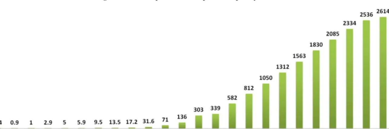
31 Figure 2.10 – Japanese wind power capacity [MW].

2.5.6 Portugal

Portugal is in the group of the tenth countries with the largest installed wind capacity with more than 4.500 MW. In 2012, Portugal became the second country with the highest wind power levels in share of domestic electricity supply (20%), just behind Denmark. The target for 2020 is 5.300 MW of installed wind power capacity, being 75 MW offshore [15]. Figure 2.11 shows the values of installed wind power capacity and the percentage of it in the local power supply.

Figure 2.11 – Portuguese wind power capacity and its share of domestic electricity supply.

(34)

32 its electricity needs from renewable sources. The wind power supplied 27% of total demand [17]-[19]. In late October, wind power covered 23% of the demanded power [20].

2.5.7 Spain

Spain is the second European country with the largest installed wind power capacity and the fourth one in the world. By the end of 2012, it counted with 22,8 GW of installed capacity and generated 48,16 TWh of energy (17,8% of national demand). The objective established for 2020 is 35.000 MW of installed wind power capacity onshore and 750 MW offshore, 29.000 MW of these must be installed by 2016 [3], [6], [21].

Since 2000, wind energy has risen dramatically, encouraged by legislation that strongly stimulated research and investment in this sector (Royal Decree 661/2007, of May 25) through premiums. After 2007 the growth has been lower due mainly to the economic crisis affecting the country. Figure 2.12 shows the values of installed wind power capacity and the percentage of it in the local power supply.

Figure 2.12 – Spanish wind power capacity and its share of domestic electricity supply.

(35)

33 production by almost 2,5 times [24]. This is a higher power (more than twice) than the generation capacity of the six existing nuclear reactors in Spain (7.742,32 MW).

2.6 FUTURE BROADCAST

Based on the 2011 and 2012 growth rates, the WWEA revised its expectations for the future global wind capacity growth, and expects a worldwide installed capacity of 500 GW by 2015. At least, 1.000 GW are expected worldwide by the end of 2020 [2], [7]. The GWEC also made their forecasts for growth in installed capacity until 2017. This forecast is lesser optimistic than the previous one and expects about 420 GW (16,26% less) of installed capacity in the world by 2015. Figure 2.13 presents installed capacity forecasts provided by the WWEA and the GWEC until 2017.

Figure 2.13 – Installed wind power capacity forecasts.

(36)

34

3 POWER SYSTEMS AND WIND TURBINES MODELS

Traditionally, power systems use synchronous machines for electricity generation. Nevertheless, in recent years the introduction of renewable energy sources like wind power, has expanded at a large rate. Such generation systems use asynchronous machines with low voltage direct current link or with electronic converters. This combination of synchronous and asynchronous generators is expected to change the power system performance and behavior following disturbances such as voltage sags and short-circuits [25].

3.1 SYSTEM ELEMENT MODELS

Due to small load changes, switching actions, and other transients are always occurring, most of the variables change with the time. Short circuits are not in steady state conditions and they can start dynamic phenomena on the system, whereby dynamic models are needed. To calculate the fault currents in the system, appropriate static models can be used. Fault currents have a transient part and a steady state one [26].

3.1.1 Loads

In power system analysis, the load can be considered as active and reactive power connected to different buses on the network model. Load can be represented by constant power, constant current or constant impedance models [27]. Among numerous devices and appliances connected to the system that are considered as loads appear distribution system feeders, shunt capacitors, transformers, voltage controlling devices, voltage regulators, etc. The model used to represent loads can be divided according to its applications in two categories: static and dynamic applications [28]. The fundamental starting point for the load modeling is at the distribution level. Thus, the applications outside of power system can be as follows:

 Static applications: this model considers only voltage dependent characteristics

o Power flow (PF)

 Harmonic power flow (HPF)

 Transmission power flow (TPF)

o Voltage stability

 Dynamic applications: considers both voltage and frequency dependent characteristics

o Transient stability (TS) o Dynamic stability (DS)

(37)

35 In this work different load models were used depending on the type of analysis to be performed as recommended in [29]. In the steady-state studies, the loads were represented by constant power models, as is usual in load flow programs. On the other hand, the dynamic studies, active power loads were represented by constant current models and reactive power loads were represented by constant impedance models.

Loads in steady-state studies

Generally, in static applications, loads are characterized considering separately the active power P and the reactive power Q. Otherwise, P and Q are represented by combining constant impedance (resistance or reactance), constant current, and constant power elements [30]. The simplest load model is the static mode and it is used for the steady-state analysis. The loads are considered like three-phase impedances connected in Y configuration modeled as constant active and reactive power as shown in Figure 3.1. In this model the load current will change when the voltage varies and it is determined by:

(2.1)

Figure 3.1 – Wye connected load for static analysis.

Author

Loads in dynamic studies

(38)

36 In this model the load current is a sum of the active component current (constant) and the reactive component, which depends of voltage variations. Thus, the load current is determinate by:

Figure 3.2 – Wye connected load for dynamic analysis.

Author

(2.2)

3.1.2 Transmission lines and transformers

Transmission lines are implemented like a balanced three-phase transmission line model with parameters lumped in a π section as shown in the Figure 3.3. In the implemented block in Simulink [31] the line parameters R, L, and C are specified as positive and zero sequence parameters ( , , , , and ) to considerate the inductive and capacitive couplings between the three phase conductors, as well as the ground parameters. This method of specifying line parameters assumes that the three phases are balanced. Self and mutual resistances ( , ), self and mutual inductances ( , ) of the coupled inductors, as well as phase capacitances and ground capacitances , are deduced from the positive and zero sequence RLC parameters as follows:

_(2.3)

_(2.4)

_(2.5)

_(2.6)

(2.7)

(39)

37 Figure 3.3 – Transmission line π model.

Author

The power transformers are the link between the generators of the power system and the transmission lines, and between lines of different voltage levels. They are highly (nearly 100%) efficient and very reliable [32]. The equivalent circuit for a single-phase transformer of the used model is showed in Figure 3.4. In this model the losses on primary and secondary windings, the losses in the core by heat, hysteresis and eddy currents are considered. Further, the inductances related to the windings, the flux in the core and the disperse flux, are also included in this model.

Figure 3.4 – Equivalent circuit for a single-phase transformer with an ideal transformer of turns ratio .

Author

3.1.3 Generators and synchronous condensers

(40)

38 each generator. The simplified model for generator and synchronous condenser are presented in Figure 3.5.

Figure 3.5 – Equivalent circuit for a single-phase generator or synchronous condenser.

Author

3.1.4 Hydraulic synchronous generator

The main objective of this work is understand and analyze the wind turbines behavior in power systems when there is high wind power penetration level and their interaction with other generators. A hydraulic plant with electrical excited synchronous generator, hydraulic turbine and excitation system was simulated to emulate the behavior and performance of the real hydraulic plants. The electrical model of the synchronous machine is represented by a sixth-order state-space model. The model considers the dynamics of the stator, field, and damper windings. The model equivalent circuit is represented in the rotor reference frame (qd frame). All rotor parameters and electrical quantities are referred to the stator. The electrical model of the machine can be found in [31] and is presented in Figure 3.6. The subscripts used are defined as follows:

 d, q: d and q axis quantities

 r, s: rotor and stator quantities

 l, m: leakage and magnetizing inductance

 f, k: field and damper winding quantity

The model equations are:

(2.9)

(2.10)

(2.11)

(2.12)

(2.13)

(2.14)

(41)

39

(2.16)

(2.17)

(2.18)

(2.19)

(2.20)

Figure 3.6 – Equivalent circuit of synchronous generator.

Author

3.1.5 Induction generators

Large-sized wind farms connected to grid are equipped with squirrel cage induction generators (SCIG), double fed induction generator (DFIG) and some synchronous generators. The most common wind turbine technology installed in systems is the DFIG. Even though few SCIG unities are still in operation, but it is not common to find them in new wind farms [33]. DFIGs have power electronics converters that can regulate their own reactive power and operate with constant power factor or constant voltage output.

Squirrel cage induction generators (SCIG)

(42)

40 reference frame (dq frame), as is shown in [31]. Figure 3.7 presents the SCIG wind power turbine used in this work.

Figure 3.7 – SCIG wind power system topology.

Author

The model equations are:

(2.21)

(2.22)

(2.23)

(2.24)

(2.25)

(2.26)

(2.27)

(2.28)

(2.29)

(2.30)

(2.31)

Figure 3.8 illustrates the electric model of an induction generator. In the SCIG the rotor voltages and (equations 2.25 and 2.27) are equal to zero.

Figure 3.8 – Equivalent circuit of the induction machine.

(43)

41 where:

, are the stator resistance and the leakage inductance; , are the magnetizing and the total stator inductances; , are the q axis voltage and current;

, are the d axis voltage and current; , are the stator q and d axis fluxes; is the reference frame angular velocity;

is angular velocity of the rotor; is the number of pole pairs;

is the electrical angular velocity ; is the electromagnetic torque;

is the total rotor inductance;

, are the rotor resistance and the leakage inductance; , are the q axis voltage and current;

, are the d axis voltage and current; and , are the stator q and d axis fluxes;

Double fed induction generator (DFIG)

With time passage, DFIGs have positioned as the most attractive technology for wind turbine manufacturers, showing themselves as an effective, economic and reliable solution. Until the mid-nineties, most of the wind turbines installed in the world were of fixed speed, using principally SCIGs and being connected to the grid directly. Thanks to technologic innovations, the panorama has changed and now most of wind turbines installed are variable speed, using DFIG [35]. In DFIG, the stator is directly connected to the grid and the rotor is feeding through a bidirectional converter, which also is connected to the grid as shown in Figure 3.9. The applied induction generator model is the same that presents Figure 3.8, with its respective equations (equations 2.21 to 2.31).

(44)

42 Figure 3.9 – DFIG wind power system topology.

Source: Kiel University, Faculty of Engineering [36].

3.2 WIND FARMS MODELS

Large wind farms are represented for investigations of transient voltage stability with two models as follow:

 Aggregated models: with representation of a turbines group in the farm with similar characteristics, with detailed representation of the internal network and the transformers connecting the generators in the internal grid.

 Reduced models: in which a large number of wind turbines contained in the farm is given by a re-scaled equivalent, e.g. one wind turbine model representing the total group of wind turbines.

Modeling details of large wind farms depends on the study purposes. In relation to transient voltage stability analysis, Akhmatov classifies in [37] the following:

1. Investigation of the mutual interaction between electricity-producing wind turbines within a large wind turbine.

2. Wind turbines response to disturbances occurred in the internal grid of the wind farm. 3. Studies of the wind farm response to short-circuit faults in the entire power system.

4. Voltage stability analysis of the power grid with large wind farms and its dynamic reactive compensation.

(45)

43 The reduced models give the wind turbines response inside the wind farm as the integrated whole. This response does not distinguish specific operational conditions or details of each wind turbine within the wind farm. Therefore, reduction to the reduced equivalent must be achieved with sufficient accuracy. Detailed examples of the aggregated model and equivalent reduced model are found in [37]-[43].

3.3 STABILITY OF SYSTEMS WITH HIGH WIND POWER LEVELS

The first studies of wind power impact on power systems date back to the early 1990s. Also, in West Denmark, the first experiences from large penetration levels occurred around this time. Several integration studies were published over the following decade with different issues and objectives. Hence, there are diverse results and conclusions. Comparisons are difficult to make owing to the approaches, results presentation and system topologies. In [3], [6] and [44] there are detailed methodologies for wind integration studies, considering economical and technical requirements as well as constraints.

So far, the integration of large wind power amounts in power systems has been studied mainly in theoretical way, because wind power penetration is still rather limited in the most countries and power systems. The main objective of power systems is to supply network customers with electricity whenever they demand for it with certain characteristics as shown in [3], [6] and [44]. So, with wind power integration the main aim must still be fulfilled.

Several works have been performed to know and understand the behavior of electrical power systems with wind farms integration. Following some of the works studied: A complete modeling and simulation of wind power systems based on the SCIG and DFIG is presented in [45]. The effect of different values of crowbar resistor in DFIGs and the effect of the DC chopper is discussed in detail in [46]. The fault ride through capability of DFIG turbines is presented in [47].

A detailed methodology to assess the impact of wind generation on the voltage stability of a power system is provided by [33]. It will also demonstrate the value of using time-series ac power ﬂow analysis techniques in assessing the behavior of a power system showing how the voltage stability margin of the power system can be increased through the proper implementation of voltage control strategies in wind turbines. Automatic procedures to generate potential contingencies based on wind power measurements and forecasts to reduce the simulation numbers and to make less complex the contingency analysis is performed in [48].

(46)

44 (STATCOM) during a fault, supporting the local voltage, while the DFIG operates as a SCIG. Conclusions about the dynamic security of non-interconnected power systems with high wind power penetration are provided in [50] and [51], considering DFIGs, permanent magnet synchronous generator (PMSG) and active stall induction generator (ASIG). Other interesting study was develop in [52], considering the introduction of electric drive vehicles (EDV) as flexible loads can improve the system operation injecting power to the system in peak hours.

3.3.1 Contradictory cases found in literature

Considering that the issue of high penetration levels of wind power in electric systems is a “novel” theme and the behavior of the system with wind generators is still in study, previous works were sought where simulations of the wind generators impact were performed. Two studies with comparative analysis of DFIGs and synchronous generators were analyzed.

The first one ([53]) concluded that synchronous generators have better performance than DFIGs for the post-fault voltage recovery. It considers a 69 Bus system with sixteen generators. The total load is , . The total power generated is , and the system losses are .

Figure 3.10 – 69 Bus system considering 16 generators.

(47)

45 Considering that statically the DFIGs do not supply as much reactive power as synchronous generators do and dynamically they cannot produce the same short circuit currents. Therefore the post-fault voltage support of a DFIG is worse than a synchronous generator. During voltage sags synchronous generators deliver more reactive current than DFIGs. For that reason synchronous generator gives better reactive power support to the grid. DFIGs consume reactive power during transient phenomena reducing the voltage stability margin.

In this study, two cases were performed. In the first one the reactive power output of the synchronous generator (G10) under faulted condition is determined, and then this synchronous generator was replaced by the same capacity DFIG and then its reactive power output was compared to that of the synchronous generator under the same operating conditions. Figure 3.11 shows the reactive power supply by the same capacity synchronous generator (G10) and DFIG during a three phase fault at the middle of line 60–61.

Figure 3.11 – Reactive power for three-phase fault at middle of one of lines 60–61

(solid line synchronous generator and dashed line DFIG).

Source: IEEE SYSTEMS JOURNAL [53].

(48)

46 Figure 3.12 – Voltage at bus 49 for three-phase fault at middle of one of lines 60–61

(solid line synchronous generator, and dashed line 60% DFIGs and 40% SGs).

Source: IEEE SYSTEMS JOURNAL [53].

In the second study ([54]) is concluded that the use of DFIGs has better performance than synchronous generators. The WSCC 3 generators 9 bus test system showed in Figure 3.13 was used with three generators and three loads, there is a large-scale wind farm based on DFIGs.

Figure 3.13 – WSCC 3-gen-9-bus test system.

Source: Power & Energy Society General Meeting, 2009 [54].

(49)

47 Figure 3.14 – Transient behavior curves of the wind farm.

Source: Power & Energy Society General Meeting, 2009 [54].

The study showed that DFIGs introduction does not affect significantly the oscillations damping time after a fault. Instead the amplitudes of the oscillations are smaller and differently shaped. The principal conclusion in this work is that DFIGs introduction could be beneficial to the system, even better than with synchronous generator, with the adequate measures.

The development of this work was based on the contrast and the conclusions of these studies, trying to analyze the impact of high penetration levels of wind power and their interaction with synchronous generators into the system. Understanding and analyzing the operational states that may have the elements of electrical systems is important to study the phenomena that can occur in them. Knowledge of stationary and transient conditions allows the sizing of protection against unwanted situations, which are responsible for the safety and reliability of the system holistically.

3.4 INFORMATICS TOOL USED

(50)

48 Figure 3.15 – Time frame of power system transients.

Author

The overall time range of power system transients is classified into fast electromagnetic transients and slow electromechanical transients. Thus, the power system is seen as a coupled electromechanical and electromagnetic system with wide range of time constants. There are fast electromagnetic transients due to the interaction between the magnetic fields of inductances and electrical fields of capacitances. Also, there are slower electromechanical transients due to the interaction between the mechanical energy stored in the rotating machines. Different time-domain simulation tools are used for studying the different dynamic phenomena in power systems.

Electromagnetic transient phenomena are usually triggered by changes in the grid configuration, as closing or opening action of circuit breakers or power electronic equipment, or by equipment failures or faults. These fast electromagnetic transients are studied with the Electromagnetic Transients Programs (EMTP) [57]. The simulation step size is of the order of tens of microseconds but can even be smaller depending on the study. Because of the long time constants associated with the dynamics of generators and turbines, simplified models of these are often sufficient for the time frame of typical electromagnetic transient’s studies.

(51)

(52)

50

4 REVIEW OF INTERNATIONAL GRID CODES FOR WIND POWER

Regulations of grid codes are defined by system operators to describe the rights and responsibilities of all generators and loads connected to the transmission and distribution systems. Due to the low wind power participation in electric systems, grid codes for wind turbines were not needed at the beginning. However, with the increased presence of wind turbines in power systems, significant penetration levels are reached.

Grid codes establishment was necessary and required to ensure the safety and reliability of the systems. The shift from conventional sources to wind power raises concerns about the impacts of large-scale wind farms on the stability of the existing electricity networks considering the fluctuating and intermittent wind power nature. To guarantee a safe grid operation, the system operators established technical requirements for large-scale wind farms. Modern grid codes provide that wind devices must remain connected to the network in case of fault and also contribute to network stability like the conventional units [58].

Although each country must adapt its grid codes according to the own characteristics of its system, such as robustness, reliability, wind power penetration level, spinning reserve, etc., there are similarities in the demanded features to generating units. With a fault occurrence somewhere in the network, the system voltages drop to the lower levels until protection units detect and isolate the affected area. As a consequence of this, wind devices terminals, as well as the other components will experience voltage sags like consequence. In the past, wind turbines could be disconnected from the network due to stability issues that can arise in case of those disturbances. An incident of this type occurred in Western Europe on November 4, 2006 when 4.892 MW of wind power were disconnected from the grid [59]. When the wind power share is important, wind farm disconnection is unacceptable. For that reason modern grid codes require the continuous operation of wind turbines under various fault conditions following some given voltage–time profiles.

(53)

51

4.1.1 Fault ride-through requirement

Low voltage ride through (LVRT) or fault ride through is the capability of electrical devices, mainly wind generators, to operate through of lower grid voltages than the operating limits. Also high voltage ride through (HVRT) exists for voltage swell conditions during which the operation above the established voltage limits is expected. Wound rotor generators designs use electrical current flowing through the windings to produce the magnetic field required for operation. These generators may have minimum and maximum working voltages, out of which they do not work properly, or have lower efficiency. Some generators will cut themselves out of the system when this situation occurs. This effect is more severe in the doubly-fed induction generators (DFIG), which have two sets of powered magnetic windings, than in squirrel-cage induction generators (SCIG) which have only one. [65].

Generation elimination by undervoltage may cause the voltage drops lower even more causing a cascading failure [66]. Modern large-scale wind turbines (1 MW and larger) require the inclusion of systems that allow them to operate during an event of this kind. Depending on the application, the generator may be required during and/or after the dip to:

 disconnect temporarily from the grid, but reconnect and continue operation after the dip

 stay operational and not disconnect from the grid

 stay connected and support the grid with reactive power

LVRT curves included in international grid codes are similar to the presented in Figure 4.1.

Figure 4.1 – Danish LVRT requirement.

(54)

52 However, depending on the regulations of each country, that curve may present some variations. Figure 4.1 shows the LVRT curve of Danish system operator where wind farms are required to withstand faults with voltage drops that reach 0,2 PU during 500 ms, followed by a voltage restoration at 0,9 PU in the next second.

Australian grid code is the most severe considering LVRT curves requiring to the wind farms withstand symmetrical and asymmetrical sags with the voltage down to zero during 100 ms and 400 ms respectively. Furthermore, the supply voltage must be restored to 0,7 PU within 2 s and to 0,8 before 10 seconds. German grid code requires ride-through capability for three-phase faults with voltage drops to zero during 150 ms, followed by the voltage recovery to 0.8 PU in 1,5 s. The old German grid code version was adopted by Ireland and USA.

LVRT curve parameters for some countries are summarized in Table 4.1. Countries like Australia, Canada, Germany, New Zealand and Spain require withstand solid faults at point of common coupling (PCC) with restoration of voltage higher to 60% in less than 2 s, being the Canadian and the Spanish grid codes the most exigent in the voltage recovery time.

Table 4.1 – LVRT requirements in international grid codes.

Grid code country

During fault Fault clearance

(PU) (s) (PU) (s)

Australia 0 0,1 0,7 2

Brazil 0,2 0,5 0,85 1

Canada 0 0,15 0,85 1

Denmark 0,2 0,5 0,9 1,5

Germany 0 0,15 0,9 1,5

Ireland 0,15 0,625 0,9 3

New Zealand 0 0,2 0,6 1

Portugal 0,2 0,5 0,8 1,5