BGD
11, 797–852, 2014Evaluating the performance of EC
CH4 analysers O. Peltola et al.
Title Page
Abstract Introduction
Conclusions References
Tables Figures
◭ ◮
◭ ◮
Back Close
Full Screen / Esc
Printer-friendly Version
Interactive Discussion
Discussion
P
a
per
|
D
iscussion
P
a
per
|
Discussion
P
a
per
|
Discuss
ion
P
a
per
|
Biogeosciences Discuss., 11, 797–852, 2014 www.biogeosciences-discuss.net/11/797/2014/ doi:10.5194/bgd-11-797-2014
© Author(s) 2014. CC Attribution 3.0 License.
Open Access
Biogeosciences
Discussions
This discussion paper is/has been under review for the journal Biogeosciences (BG). Please refer to the corresponding final paper in BG if available.
Evaluating the performance of commonly
used gas analysers for methane eddy
covariance flux measurements: the
InGOS inter-comparison field experiment
O. Peltola1, A. Hensen2, C. Helfter3, L. Belelli Marchesini4, F. C. Bosveld5, W. C. M. van den Bulk2, J. A. Elbers6, S. Haapanala1, J. Holst7, T. Laurila8, A. Lindroth7, E. Nemitz3, T. Röckmann9, A. T. Vermeulen2, and I. Mammarella1
1
Department of Physics, University of Helsinki, Helsinki, Finland
2
Energy Research Centre of the Netherlands, Petten, the Netherlands
3
Centre for Ecology and Hydrology, Edinburgh research station, Penicuik, UK
4
Department of Earth Sciences, VU University, Amsterdam, the Netherlands
5
Royal Netherlands Meteorological Institute, De Bilt, the Netherlands
6
Alterra, Wageningen, the Netherlands
7
Department of Physical Geography and Ecosystem Science, Lund University, Lund, Sweden
8
Finnish Meteorological Institute, Helsinki, Finland
9
BGD
11, 797–852, 2014Evaluating the performance of EC
CH4 analysers O. Peltola et al.
Title Page
Abstract Introduction
Conclusions References
Tables Figures
◭ ◮
◭ ◮
Back Close
Full Screen / Esc
Printer-friendly Version
Interactive Discussion
Discussion
P
a
per
|
D
iscussion
P
a
per
|
Discussion
P
a
per
|
Discuss
ion
P
a
per
|
Received: 20 December 2013 – Accepted: 26 December 2013 – Published: 13 January 2014
Correspondence to: O. Peltola ([email protected])
BGD
11, 797–852, 2014Evaluating the performance of EC
CH4 analysers O. Peltola et al.
Title Page
Abstract Introduction
Conclusions References
Tables Figures
◭ ◮
◭ ◮
Back Close
Full Screen / Esc
Printer-friendly Version
Interactive Discussion
Discussion
P
a
per
|
D
iscussion
P
a
per
|
Discussion
P
a
per
|
Discuss
ion
P
a
per
|
Abstract
The performance of eight fast-response methane (CH4) gas analysers suitable for eddy covariance flux measurements were tested at a grassland site near the Cabauw tall tower (Netherlands) during June 2012. The instruments were positioned close to each other in order to minimize the effect of varying turbulent conditions. The moderate CH4
5
fluxes observed at the location, of the order of 25 nmol m−2s−1, provided a suitable signal for testing the instruments’ performance.
Generally, all analysers tested were able to quantify the concentration fluctuations at the frequency range relevant for turbulent exchange and were able to deliver high-quality data. The tested cavity ring-down spectrometer (CRDS) instruments from
Pi-10
carro, models G2311-f and G1301-f, were superior to other CH4analysers with respect to instrumental noise. As an open-path instrument susceptible to the effects of rain, the LI-COR LI-7700 achieved lower data coverage and also required larger density cor-rections; however, the system is especially useful for remote sites that are restricted in power availability. In this study the open-path LI-7700 results were compromised due
15
to a data acquisition problem in our data-logging setup. Some of the older closed-path analysers tested do not measure H2O vapour concentrations alongside CH4(i.e. FMA1 and DLT-100 by Los Gatos Research) and this complicates data processing since the required corrections for dilution and spectroscopic interactions have to be based on external information. To overcome this issue, we used H2O mole fractions measured
20
by other gas analysers, adjusted them with different methods and then applied them to correct the CH4 fluxes. Following this procedure we estimated a bias on the order of 0.1 g (CH4) m−2(8 % of the measured mean flux) in the processed and corrected CH4 fluxes on a monthly scale due to missing H2O concentration measurements. Finally, cumulative CH4fluxes over 14 days from three closed-path gas analysers, G2311-f
(Pi-25
carro Inc.), FGGA (Los Gatos Research) and FMA2 (Los Gatos Research), which were measuring H2O vapour concentrations in addition to CH4, agreed within 3 % (355– 367 mg (CH4) m
−2
BGD
11, 797–852, 2014Evaluating the performance of EC
CH4 analysers O. Peltola et al.
Title Page
Abstract Introduction
Conclusions References
Tables Figures
◭ ◮
◭ ◮
Back Close
Full Screen / Esc
Printer-friendly Version
Interactive Discussion
Discussion
P
a
per
|
D
iscussion
P
a
per
|
Discussion
P
a
per
|
Discuss
ion
P
a
per
|
instruments derived total fluxes which showed small but distinct differences (±10 %, 330–399 mg (CH4) m
−2 ).
1 Introduction
Methane (CH4) is the third most important greenhouse gas, after water (H2O) and carbon dioxide (CO2). Due to its high global warming potential of 25 (at the 100 yr
hori-5
zon) changes in its abundance have an effect on the on-going climate change. The total global methane source is thought to be relatively well-quantified, but the relative contributions of each source and changes in individual sources are not (Forster et al., 2007). The gradual increase in atmospheric methane concentration observed over the last century decreased in the past decades and came to a standstill around 2000 for
10
several years before starting to increase again since 2007 (Dlugokencky et al., 2011). Explanations for the temporary standstill are inconsistent with each other, highlight-ing the need for improved bottom-up inventories to understand better the most impor-tant factors controlling the changes in atmospheric methane (Heimann, 2011). Several mechanisms have been proposed to explain the temporary decline in the growth rate,
15
such as (a) decreases in anthropogenic emissions (e.g. Dlugokencky et al., 1994), (b) decreases in anthropogenic emissions before 1999, and decreases in wetland emis-sions after that (Bousquet et al., 2006) or (d) changes in the removal rate by OH (e.g. Monteil et al., 2011). A network of eddy covariance (EC) towers can provide direct and continuous monitoring of ecosystem scale surface fluxes that can be upscaled to
land-20
scape and continental scales using process-based models. This combined approach can help unravelling the relative contribution of different sources and sinks on global methane budget.
Over the last 20 yr, thanks to advancements in laser absorption spectroscopy (LAS), several methane gas analysers suitable for eddy covariance measurements have been
25
BGD
11, 797–852, 2014Evaluating the performance of EC
CH4 analysers O. Peltola et al.
Title Page
Abstract Introduction
Conclusions References
Tables Figures
◭ ◮
◭ ◮
Back Close
Full Screen / Esc
Printer-friendly Version
Interactive Discussion
Discussion
P
a
per
|
D
iscussion
P
a
per
|
Discussion
P
a
per
|
Discuss
ion
P
a
per
|
and they also had relatively high flux detection limits (e.g. Fowler et al., 1995). This made long-term measurements challenging and time consuming and inhibited mea-surements at remote locations which are often important methane sources, such as remote wetlands in Siberia and North America. After development of gas analysers that can use peltier cooling systems, measurements became possible at these remote
5
locations, although availability of mains power remained an issue. Recently, a new generation of commercial fast-response CH4 sensors has become available which of-fers a much improved signal/noise ratio and is even easier to use due to stable op-eration. Consequently there are large efforts to create continental scale networks of measurement stations (e.g. Integrated Carbon Observation System (ICOS) and
Inte-10
grated non-CO2Greenhouse gas Observing System (InGOS)) allowing for CH4fluxes to be measured continuously. In this context, it is important to characterise the currently available CH4analysers and assess their performance. A few inter-comparison studies exist (Detto et al., 2011; Peltola et al., 2013; Tuzson et al., 2010), but none of them included such a wide range of models currently available on the market as this study.
15
This study reports results from an inter-comparison experiment held at a Dutch grassland site in June 2012 as part of the InGOS (Integrated non-CO2 Greenhouse gas Observing System) EU-FP7 project. The objective of this study was to evaluate the field performance of the instruments tested, to determine the accuracy and preci-sion of the measured fluxes and to assess the relative merits of different instrumental
20
designs (e.g. open vs. closed path gas analysers). This presentation of the results ad-dresses the following topics in detail: (i) precision of CH4measurements from each in-strument; (ii) an analysis of the impact of corrections due to density fluctuations (WPL) and spectroscopic effects on the fluxes; (iii) an evaluation of the errors arising when external H2O signal is used for the WPL and spectroscopic corrections of the CH4flux
25
BGD
11, 797–852, 2014Evaluating the performance of EC
CH4 analysers O. Peltola et al.
Title Page
Abstract Introduction
Conclusions References
Tables Figures
◭ ◮
◭ ◮
Back Close
Full Screen / Esc
Printer-friendly Version
Interactive Discussion
Discussion
P
a
per
|
D
iscussion
P
a
per
|
Discussion
P
a
per
|
Discuss
ion
P
a
per
|
2 Experimental setup
2.1 Site
The gas analyser inter-comparison experiment was performed at the Cabauw Ex-perimental Site for Atmospheric Research (CESAR) (51◦58′12.00′′N, 4◦55′34.48′′E, −0.7 m a.s.l.). The Cabauw tall tower combines a comprehensive set of observations to
5
profile many aspects of the atmospheric column (www.cesar-observatory.nl). A broad range of atmospheric and ecological measurements are conducted on a continuous basis. The site is located in an agricultural landscape, with methane emissions origi-nating from ruminants and other agricultural activities, but also from the peaty soil and the drainage ditches between the surrounding fields. The soil consists of a 0.5 to 1 m
10
deep clay layer on top of a peat layer which is several meters deep. The water table level is on average 0.5 m below the surface. For a more thorough site description, see e.g. Beljaars and Bosveld (1997) and van Ulden and Wieringa (1996).
During the campaign, the vegetation surrounding the measurement tower was low (0.05–0.2 m) although a taller maize field was located 70 m away in SW–W direction
15
from the measurement mast (see Fig. 1). The landscape is relatively flat and level, making the area ideal for micrometeorological flux measurements. The eddy covari-ance measurement tower was approximately 87 m away from the nearest building, the Cabauw tall tower (height 213 m), located to the NE. The fetch in the main wind direc-tion (W–SW) was free from any large obstacles for several hundreds of metres.
20
Meteorological conditions during the campaign were recorded next to the measure-ment mast by a weather station operated by the Royal Netherlands Meteorological Institute (KNMI). Air temperature during the campaign ranged between 4.3 and 22.0◦C with an average of 14.9◦C. Rain was recorded on 19 out of 22 measurement days, 21 June being the rainiest day with a total of 14.1 mm of rain. Cumulative rainfall during
25
BGD
11, 797–852, 2014Evaluating the performance of EC
CH4 analysers O. Peltola et al.
Title Page
Abstract Introduction
Conclusions References
Tables Figures
◭ ◮
◭ ◮
Back Close
Full Screen / Esc
Printer-friendly Version
Interactive Discussion
Discussion
P
a
per
|
D
iscussion
P
a
per
|
Discussion
P
a
per
|
Discuss
ion
P
a
per
|
2.2 Measurement system
Eddy covariance flux measurements were conducted between 6 and 27 June 2012 at a 6.5 m high tower. Two sonic anemometers were used (both USA-1, METEK, Ger-many) to acquire fast measurements of wind velocity components and sonic tempera-ture. Similar instruments were used in an effort to minimize the potential systematic bias
5
on CH4 fluxes caused by the use of different types of anemometers. The anemome-ters were placed on the same tower at the same height with approximately one meter horizontal distance in NW–SE direction between them (see Fig. 1).
All data were logged at a frequency of 20 Hz by a central computer located in a trailer that also housed the closed-path analysers. The trailer was approximately 26 m away
10
from the measurement tower in the NE direction. The trailer was air conditioned and the indoor temperature was kept around 22◦C. Data logging software capable of handling and saving all 56 variables at 20 Hz was written in LabView for this campaign (National Instruments, USA).
The gas analysers were divided between the two anemometers which will from now
15
on be referred to as METEK1 and METEK2. Two open-path analysers (Models LI-7500 and LI-7700, LI-COR Biogeosciences, USA) were situated on both sides of METEK1, displaced in NW–SE direction by approximately 0.3 m. The LI-7500 measured CO2 and H2O mole densities, while the LI-7700 measured CH4. Two separate LI-7700 anal-ysers were used sequentially and the switch between instruments was done at 19th
20
of June. The LI-7700 is a low-power, lightweight methane gas analyser with a 0.8 m long open measurement cell. Its operation principle is based on laser absorption spec-troscopy, more precisely wavelength modulation spectroscopy (McDermitt et al., 2010). The LI-7700 reports CH4 molar density (mmol m
−3
) while all the other CH4 analy-sers report mole fraction (ppm). Unfortunately the data were recorded with three
dec-25
BGD
11, 797–852, 2014Evaluating the performance of EC
CH4 analysers O. Peltola et al.
Title Page
Abstract Introduction
Conclusions References
Tables Figures
◭ ◮
◭ ◮
Back Close
Full Screen / Esc
Printer-friendly Version
Interactive Discussion
Discussion
P
a
per
|
D
iscussion
P
a
per
|
Discussion
P
a
per
|
Discuss
ion
P
a
per
|
more attenuated and noisier than normal (cf. Fig. 5h below). This data logging problem should be kept in mind for the interpretation of the results of this study.
In addition to the two open-path devices, three closed-path gas analysers (G2311-f, Picarro Inc., USA; FGGA, Los Gatos Research, USA; DLT-100, Los Gatos Research, USA) were sampling from METEK1 (the sampling setup of all gas analysers is
de-5
scribed in Table 1). The G2311-f is a new gas analyser by Picarro Inc. and is based on cavity ringdown spectroscopy (CRDS). The analyser is able to make simultane-ous fast measurements of CO2, CH4 and H2O mole fractions. The whole sampling line connected to the G2311-f was heated in order to prevent condensation of water on the tube walls. The FGGA (“Fast Greenhouse Gas Analyser”) developed by Los
10
Gatos Research is based on off-axis integrated cavity output spectroscopy (OA-ICOS) and the instruments provide fast measurements of CO2, CH4 and H2O mole fractions on a continuous basis. The FGGA tested is the standard (rack-mount) version rather than the later introduced enhanced performance version with more accurate temper-ature control. The third closed-path analyser accompanying METEK1 was a DLT-100,
15
an older benchtop model (production year: 2005) by Los Gatos Research. It is based on the same measurement principle as the FGGA (OA-ICOS); however, it is able to measure and report mole fractions only of CH4. Until 16th of June the instrument mea-sured reported data at 1 Hz and after that the sampling frequency of this instrument was set to 10 Hz. This was taken into account when spectral corrections were applied
20
(Sect. 4.3.1.).
Five closed-path gas analysers sampled from near METEK2. Four of them measured CH4and one only CO2 and H2O. These four methane analysers were: a G1301-f (Pi-carro Inc., USA), a QCL (Aerodyne Research Inc., USA) and two FMAs (Los Gatos Research, USA). Henceforth, the two rackmount FMAs are referred to as FMA1 and
25
BGD
11, 797–852, 2014Evaluating the performance of EC
CH4 analysers O. Peltola et al.
Title Page
Abstract Introduction
Conclusions References
Tables Figures
◭ ◮
◭ ◮
Back Close
Full Screen / Esc
Printer-friendly Version
Interactive Discussion
Discussion
P
a
per
|
D
iscussion
P
a
per
|
Discussion
P
a
per
|
Discuss
ion
P
a
per
|
capable of measuring any two out of three gases (CH4, CO2and H2O) simultaneously. During this campaign the instrument was not able to measure H2O and thus CH4and CO2were selected. The QCL is an older (pulsed) quantum cascade laser by Aerodyne Research Inc. The detector was cooled with liquid nitrogen using an automated LN2 filling system. During this campaign, the QCL measured both CH4and N2O. A Perma
5
Pure drier was connected to the QCL sampling line in order to remove H2O from the air samples. The Fast Methane Analyser (FMA) is a slightly older model by Los Gatos Research using OA-ICOS. The standard FMA instrument is able to measure and report only CH4mole fractions but it can be updated to measure also H2O. While FMA1 was a standard CH4instrument, FMA2 was upgraded to enable the parallel H2O
measure-10
ments. The LI-7000 (LI-COR Biogeosciences, USA) was used to measure CO2 and H2O from the vicinity of METEK2. These water measurements were needed for the corrections applied to some of the CH4fluxes (Sect. 3).
3 Data post-processing
3.1 Introduction
15
Under the assumptions of turbulence stationarity, horizontally homogeneous surface and turbulence characteristics, the mass balance equation is reduced into a simple form which is the basis of eddy covariance measurements:
Fc=
ρd
Md
w′r′
c (1)
Where Fc is the flux of gas c at the surface, ρd is mean dry air density, Md is the
20
BGD
11, 797–852, 2014Evaluating the performance of EC
CH4 analysers O. Peltola et al.
Title Page
Abstract Introduction
Conclusions References
Tables Figures
◭ ◮
◭ ◮
Back Close
Full Screen / Esc
Printer-friendly Version
Interactive Discussion
Discussion
P
a
per
|
D
iscussion
P
a
per
|
Discussion
P
a
per
|
Discuss
ion
P
a
per
|
concentration relative to moist air (i.e. mole fraction,χc), or in the case of open-path analysers the gas mass density (ρc), which is affected by fluctuations in temperature and humidity. In addition, the instruments used to measure gas concentrations and wind components are non-ideal, i.e. they do not make truly instantaneous measure-ments and therefore act as bandpass filters effectively filtering out certain high and low
5
frequencies in the signal. Both of these effects need to be corrected, in addition to other post-processing steps, before the measured flux represents the flux at the surface. The correction methods used in this study are discussed in greater detail in the following sections.
3.2 General data post-processing steps
10
Data obtained during the campaign was post-processed with EddyUH software (freely available at http://www.atm.helsinki.fi/Eddy_Covariance/index.php). The post-processing steps followed generally adopted methods by Aubinet et al. (2000) and they were organized as follows:
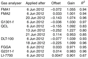
– First the CH4 time series were converted with calibration parameters (Table 2)
15
from measured ppm (mmol m−3 for LI-7700) to calibrated units. The parameters were obtained with the method described in Sect. 3.3.
– The raw eddy covariance data were despiked by comparing two temporally adja-cent CH4concentration measurements. If their difference was larger than 3 ppm the following point was considered a spike and was replaced with the value of the
20
BGD
11, 797–852, 2014Evaluating the performance of EC
CH4 analysers O. Peltola et al.
Title Page
Abstract Introduction
Conclusions References
Tables Figures
◭ ◮
◭ ◮
Back Close
Full Screen / Esc
Printer-friendly Version
Interactive Discussion
Discussion
P
a
per
|
D
iscussion
P
a
per
|
Discussion
P
a
per
|
Discuss
ion
P
a
per
|
– For closed-path instruments which measured also H2O the effect of fluctuating humidity on methane concentration measurements were corrected point-by-point according to Eq. (4) below, with coefficients given in Table 3.
– The coordinate system of the sonic anemometer was rotated using the double rotation method (Rebmann et al., 2012), aligning the x-axis of the anemometer
5
with the mean flow.
– Linear detrending was used to separate the turbulent signal from the measure-ments, and the covariances were calculated by searching the maximum of the cross-covariance function within certain predefined lag windows. A 30 min aver-aging period was used for all fluxes.
10
– Within an iterative loop, the rest of CH4 fluxes were corrected for the effect of fluctuating humidity and also for fluctuating temperature for open-path LI-7700 (Sect. 3.4). Temperature fluctuations are expected to be fully damped by the time the sample reaches the closed-path instrument.
– Finally, the fluxes were corrected for high and low frequency damping, based on
15
the method described by Aubinet et al. (2000).
The overall correction factor CF used to correct for band-pass filtering was calculated as
CF=
∞
R
0
Cmod(f)df
∞
R
0
TFLF(f)TFHF(f)Cmod(f)df
(2)
where TFLF is a transfer function describing low frequency dampening, adopted from
20
BGD
11, 797–852, 2014Evaluating the performance of EC
CH4 analysers O. Peltola et al.
Title Page
Abstract Introduction
Conclusions References
Tables Figures
◭ ◮
◭ ◮
Back Close
Full Screen / Esc
Printer-friendly Version
Interactive Discussion
Discussion
P
a
per
|
D
iscussion
P
a
per
|
Discussion
P
a
per
|
Discuss
ion
P
a
per
|
determined by fitting a curve to ensemble averaged temperature cospectra.T FHFwas determined experimentally by fitting the Lorentzian function (Eq. 3), which is based on a first-order recursive filter (Eugster and Senn, 1995), to the ratio between measured CH4and temperature cospectra.
TFHF= 1
1+(2πf τ)2 (3)
5
τ is a measurement system specific fit parameter which characterises the high fre-quency filtering effects.
3.3 Calibration coefficients
The analysers had not been calibrated against common standards prior to the start of the inter-comparison exercise. In order to minimize the differences in the CH4 fluxes
10
caused by different calibrations, the following procedure was applied: 30 min mean val-ues for the concentrations were calculated for each methane concentration time series. These values were compared with high precision measurements (calibrated against the NOAA2004 concentration scale) made at 20 m height at the CESAR tower with another G2301 instrument (Picarro Inc., USA). Only daytime periods (between 9:00 LT
15
and 21:00 LT) when CH4concentration difference between 20 m and 60 m heights was smaller than 15 ppb were used. Under such circumstances, the concentrations mea-sured at 20 m and 6.5 m heights were assumed to be sufficiently similar. A simple linear regression between 20 m height measurements and CH4time series derived from EC measurements was used to obtain the calibration parameters (offset and gain)
(Ta-20
ble 2) for each EC methane time series. For the QCL three sets of coefficients were determined since the fitting procedure of the instrument was changed two times during the campaign and this had an effect on the reported CH4 values. For the FMA2 and DLT-100 two sets of coefficients were determined: for FMA2 the calibration changed since the sampling cell was cleaned and for the DLT-100 it changed due to
BGD
11, 797–852, 2014Evaluating the performance of EC
CH4 analysers O. Peltola et al.
Title Page
Abstract Introduction
Conclusions References
Tables Figures
◭ ◮
◭ ◮
Back Close
Full Screen / Esc
Printer-friendly Version
Interactive Discussion
Discussion
P
a
per
|
D
iscussion
P
a
per
|
Discussion
P
a
per
|
Discuss
ion
P
a
per
|
ing the instrument which caused a sudden decrease in the cavity ringdown time and consequently a slight change in calibration.
3.4 Corrections for density and spectroscopic effects
Humidity and temperature fluctuations affect gas flux measurements by causing changes in air density (Webb et al., 1980; Massman and Tuovinen, 2006; Ibrom et al.,
5
2007) and, for gas analysers based on laser absorption spectrometry, also by altering the shape of gas absorption line (McDermitt et al., 2010; Neftel et al., 2010; Tuzson et al., 2010). Corrections for these effects are referred to as density and spectroscopic correction, respectively.
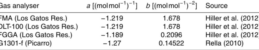
Rella (2010) proposed to correct both of these effects for closed-path gas analysers
10
by using a second order polynomial function
χc=rc
1+aχv+bχv2
(4)
whereχcis the molar fraction of gasc,rc is the mixing ratio of gasccorrected for any interference from water,χvthe water vapour molar fraction andaandbare instrument specific coefficients which describe the dependence of χc onχv. This expression has
15
been demonstrated to be suitable for correcting measurements for dilution and spec-troscopic effects in several studies (Chen et al., 2010; Hiller et al., 2012; Nara et al., 2012; Rella et al., 2013), and it is nowadays widely used. It is worth noting that Eq. (4) is reduced to the correction for dilution alone (i.e. density correction for closed- path gas analysers) fora=−1 andb=0. This form of correction is easily applicable if the
20
gas analyser measures both,χc and χv, and in fact is implemented into some of the instruments that can thus report a dry mixing ratio (e.g. G2311-f, which uses coeffi -cients from Chen et al., 2010). However, some of the laser spectrometers used in this study did not measure water and thus external water measurements were needed to correct the gas measurements. When using external water measurements, it may be
25
BGD
11, 797–852, 2014Evaluating the performance of EC
CH4 analysers O. Peltola et al.
Title Page
Abstract Introduction
Conclusions References
Tables Figures
◭ ◮
◭ ◮
Back Close
Full Screen / Esc
Printer-friendly Version
Interactive Discussion
Discussion
P
a
per
|
D
iscussion
P
a
per
|
Discussion
P
a
per
|
Discuss
ion
P
a
per
|
the external and internal χv are not passed on to the high frequencyχc time series. By using Reynolds decomposition, averaging and slightly reorganizing the terms, the expression above can be converted into flux form (see Appendix A for derivation):
Fc=
ρa
Ma
1−χv
1+aχv+bχv 2
w
′χ′
c+
χc
1−χv w′χ′
v−
a+2bχv−bχv
2
+1
1+aχv+bχv 2
1−χv
χcw′χv′
= 1−χv
1+aχv+bχv 2
FcRAW+FcWPL+FcSPECT
(5)
5
whereρais the mean total air density andMais the mean molar mass of moist air. The first term on the right hand side is the measured flux (FcRAW), the second term is the effect of air density fluctuations (FcWPL, H2O term in WPL correction) and the third term (FcSPECT) and the multiplier in front of the parentheses arise from the spectroscopic
10
effects that water vapour has on the measurements of gasc.
One should note that Eq. (5) is identical to Eq. (3a) in Ibrom et al. (2007) if we take
a=−1 andb=0, meaning that the spectroscopic effects are neglected, and only the effect of density fluctuations is corrected. In addition, it should be emphasized that in normal circumstances the two correction methods presented above (Eqs. 4 and 5)
15
will deliver the same result, if and only if the water vapour covariance, w′χ′
v, reflects the variation in water vapour concentration in the measurement cell when gas c is measured, a point which has been highlighted for density correction (Ibrom et al., 2007; Massman, 2004). This applies also to spectroscopic correction and to the combined correction of Eq. (5).
20
BGD
11, 797–852, 2014Evaluating the performance of EC
CH4 analysers O. Peltola et al.
Title Page
Abstract Introduction
Conclusions References
Tables Figures
◭ ◮
◭ ◮
Back Close
Full Screen / Esc
Printer-friendly Version
Interactive Discussion
Discussion
P
a
per
|
D
iscussion
P
a
per
|
Discussion
P
a
per
|
Discuss
ion
P
a
per
|
G1301-f and DLT-100), the correction was performed using Eq. (5), and the water vapour covariance,w′χ′
v, was adjusted using the empirical procedure described below (Sect. 3.4.1). For FMA1 it was performed using Eq. (5) and the water vapour covari-ance from the LI-7000,w′χ′
v, calculated with FMA1 CH4lag time because LI-7000 and FMA1 shared the same inlet line. CH4signals from the G2311-f and the QCL were free
5
from H2O interference since the G2311-f applied a similar correction internally during the measurements and the QCL was connected to a drier. Open-path gas analyser LI-7700 methane measurements are not only affected by the water vapour concentration, but also by temperature fluctuations, and these resulting CH4 fluxes were corrected with the method proposed by McDermitt et al. (2010).
10
3.4.1 Using external H2O in correcting CH4fluxes
Adsorption/desorption of H2O molecules on the sampling tube walls and filters (closed-path gas analysers only) cause amplitude and phase shifts compared to an unper-turbed, ideal signal (Fratini et al., 2012; Ibrom et al., 2007; Mammarella et al., 2009; Massman and Ibrom, 2008; Nordbo et al., 2013). Thus, H2O lag times tend to be longer
15
than for other gases in the same sampling tube and attenuations of H2O fluctuations are enhanced. Adsorption/desorption of H2O depends on sampling line characteris-tics, i.e., tube material, flow rate, filter etc. Moreover the mechanisms are enhanced when relative humidity increases and/or dirt accumulates on the wall of the tube. This enhancement is sampling line specific (Ibrom et al., 2007; Mammarella et al., 2009).
20
To date a comprehensive explanation for the amplitude and phase shifts is missing; however Nordbo et al. (2013) showed promising development in this aspect.
A problem arises from the fact that attenuation and phase shift of H2O are not known in the sampling lines of those gas analysers not capable of measuring H2O. Thus, correcting CH4 data for the H2O effect is difficult. To partly overcome these diffi
cul-25
BGD
11, 797–852, 2014Evaluating the performance of EC
CH4 analysers O. Peltola et al.
Title Page
Abstract Introduction
Conclusions References
Tables Figures
◭ ◮
◭ ◮
Back Close
Full Screen / Esc
Printer-friendly Version
Interactive Discussion
Discussion
P
a
per
|
D
iscussion
P
a
per
|
Discussion
P
a
per
|
Discuss
ion
P
a
per
|
parameterized as a function of RH:
tH2O
tCO2 =
c+d
RH 100
e
, (6)
where RH is relative humidity in %. Data were grouped in 12 relative humidity classes and the fit parametersc,d andewere obtained by fitting the above expression to me-dian values in the 12 relative humidity classes (r2=0.9963 and RMSE=0.0841),
yield-5
ing the values c=1.081 (95 % confidence bounds: 1.002–1.159), d=6.369 (5.849– 6.888) ande=14.06 (12.43–15.69). Then it was assumed that the ratio has the same relative humidity dependence in all sampling lines and, finally, the water vapour covari-ance,w′χ′
v, used in Eq. (5) was calculated with a lag time of
t=tANA2H
2O
−
c+d
RH
100
e
tCHANA1
4
−tANA1 CH4
t=tANA2H
2O
−∆t
, (7)
10
wheretANA2H
2O is lag time of H2O measured with for instance LI-7000 andt
ANA1
CH4 is lag time of CH4measured with for instance FMA.∆ttakes into account the phase shift between H2O and CH4in the sampling line. Now, instead of calculatingw′χ
′ v witht
ANA2
H2O , which corresponds to maximizing the covariance, the covariance is calculated withtand then
15
Eq. (5) was applied. No attempt was made to correct for differences in attenuation of H2O in different sampling lines. Moreover, the assumption that the ratio between H2O and CO2lag times follows the same relative humidity dependence in all sampling lines may not necessarily be valid.
3.5 Random errors in the flux
20
BGD
11, 797–852, 2014Evaluating the performance of EC
CH4 analysers O. Peltola et al.
Title Page
Abstract Introduction
Conclusions References
Tables Figures
◭ ◮
◭ ◮
Back Close
Full Screen / Esc
Printer-friendly Version
Interactive Discussion
Discussion
P
a
per
|
D
iscussion
P
a
per
|
Discussion
P
a
per
|
Discuss
ion
P
a
per
|
2010), caused by the stochastic nature of turbulence, rather than the performance of the instrument used in the measurement. In this study, the total random uncertainty of a flux estimate is calculated with the method proposed by Finkelstein and Sims (2001). In this method, the error variance of the covariance is estimated based on cross-covariances and auto-covariances and thus the uncertainty estimate contains
5
contributions originating from sampling uncertainty and instrumental noise.
Lenschow et al. (2000) introduced a method to estimate instrumental noise in LiDAR measurements and later Mauder et al. (2013) applied it to eddy covariance data. Due to the fact that instrumental noise is uncorrelated with the turbulent signal, it can be assumed that the noise contributes to the auto-covariance only at lag zero. Thus, the
10
instrumental noise can be estimated as the difference between the observed value of auto-covariance at lag zero (i.e. variance of the time series) and extrapolation of auto-covariance function values to lag zero:
σcnoise2=C11(0)−C11(p→0), (8)
whereC11=C11(p) is the auto-covariance function,pis the lag and C11(p→0) is the
15
extrapolation of auto-covariance function to lag zero.C11(p→0) was estimated using linear extrapolation and auto-covariance values at lags 4≤p≤11 were used for the extrapolation. In essence, with this method the observed variance of time seriesC11(0) is divided into two parts: variance caused by turbulent mixing,C11(p→0), and variance caused by instrumental noise (σcnoise)2. Therefore, σcnoise describes the noise level in
20
the measured time series. Contribution of this noise to uncertainty of the covariance is estimated using error propagation (Eq. 7 in Mauder et al., 2013):
σw,noisec = v u u t
σcnoise2σw2
N (9)
whereN is the amount of samples in a time series andσw2 is variance of vertical wind component. Unlike in the original equation given in Mauder et al. (2013), the
BGD
11, 797–852, 2014Evaluating the performance of EC
CH4 analysers O. Peltola et al.
Title Page
Abstract Introduction
Conclusions References
Tables Figures
◭ ◮
◭ ◮
Back Close
Full Screen / Esc
Printer-friendly Version
Interactive Discussion
Discussion
P
a
per
|
D
iscussion
P
a
per
|
Discussion
P
a
per
|
Discuss
ion
P
a
per
|
tion of instrumental noise in w was neglected since the focus was on comparing the gas analysers. This method is sensitive only to random noise, i.e. white noise, in the signal and it cannot be used to estimate drift or low frequency noise in the signal, since such variations contribute to auto-covariance at multiple lag times, not just at lag zero. Eddy covariance fluxes are usually estimated by maximizing the cross-covariance
5
between time seriesw and χc. Wienhold et al. (1995) developed a method to assess how well this maximum can be detected from the cross-covariance. In their method the detection limit of a flux is estimated as the standard deviation of the cross-covariance function values far from the maximum value, i.e. the flux. In essence, this method esti-mates the magnitude of the background variation of the cross-covariance. In this study
10
the detection limits were estimated by using the position of the maximum as the origin of time, calculating the cross-covariance between time seriesw andχcwithin lag win-dows−150 s to −50 s and 50 s to 150 s, and finally calculating the standard deviation of the obtained values cross-covariance values.
3.6 Flux data filtering and quality control
15
The flux data were screened in order to remove clearly erroneous values. Flux data were removed if there were too many spikes during an averaging period (over 3000 spikes), 30 min mean CH4 concentrations were unrealistic (below 1.7 ppm or above 3.5 ppm) or sonic anemometer data were erroneous. In addition, the open-path LI-7700 data were screened based on the RSSI (Received signal strength indicator) and
20
the diagnostic value provided by the instrument. The diagnostic value describes instru-ment activities during operation and RSSI represents how clean the mirrors in the open measurement cell are. Periods were omitted, if the 30 min mean value for RSSI was below 15. Periods were also rejected if no laser signal was detected for more than 5 % of the time, or if over 3 % of time the lower mirror spin motor was on. In addition to
25
BGD
11, 797–852, 2014Evaluating the performance of EC
CH4 analysers O. Peltola et al.
Title Page
Abstract Introduction
Conclusions References
Tables Figures
◭ ◮
◭ ◮
Back Close
Full Screen / Esc
Printer-friendly Version
Interactive Discussion
Discussion
P
a
per
|
D
iscussion
P
a
per
|
Discussion
P
a
per
|
Discuss
ion
P
a
per
|
were distributed into three quality classes based on a flux stationarity test (Foken and Wichura, 1996). If the test yielded smaller values than 0.3, the fluxes were given qual-ity flag 0 (highest qualqual-ity), fluxes with test values between 0.3 and 1 were given flag 1 (medium quality) and if the test yielded values above 1, then the fluxes were flagged with 2 (low quality).
5
4 Results
4.1 Data coverage and quality
The poorest data coverage (Fig. 2) was obtained with the G1301-f and DLT-100 in-struments (26.7 % and 64.4 %, respectively); however this was caused by data logging problems and does not reflect instrument performance. FGGA and G2311-f achieved
10
the best data coverage, which also had often the high quality flag (Fig. 3).
The largest data filtering effect using screening procedure described in Sect. 3.6 was for the LI-7700, with approximately 43 % of data rejected. This was mainly related to one period (from 9 to 14 June 2012) during which both mirrors became dirty and manual cleaning was not possible. From 18 June onwards the mirrors were cleaned
15
manually every second day. The friction velocity criterion removed 66 30 min CH4 flux data points (6 % of data) from all time series.
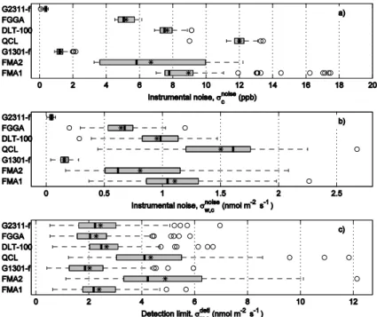
4.2 Random errors and instrumental noise
The statistics of the estimates for instrumental noise levels are shown for each instru-ment in Fig. 4 for periods when all gas analysers were working. The noise was not
20
estimated for the LI-7700 due to the data logging problem (explained in Sect. 2.2). On average, the two Picarro analysers, G2311-f and G1301-f, had the lowest instrumental noise (0.4 ppb and 1.2 ppb, respectively) during the study period (Fig. 4a and b). It is however questionable whether the method used can adequately separate the turbulent signal from the instrumental noise in the case of the G2311-f for which the overall noise
BGD
11, 797–852, 2014Evaluating the performance of EC
CH4 analysers O. Peltola et al.
Title Page
Abstract Introduction
Conclusions References
Tables Figures
◭ ◮
◭ ◮
Back Close
Full Screen / Esc
Printer-friendly Version
Interactive Discussion
Discussion
P
a
per
|
D
iscussion
P
a
per
|
Discussion
P
a
per
|
Discuss
ion
P
a
per
|
level was very small. For comparison, the standard deviations of CH4 concentrations, which contain contributions from both instrumental noise and atmospheric fluctuations, measured by the two Picarro instruments were approximately 4.6 ppb and 4.3 ppb, re-spectively. Thus the variations in the methane time series from these two analysers were clearly dominated by atmospheric fluctuations, rather than instrumental noise.
5
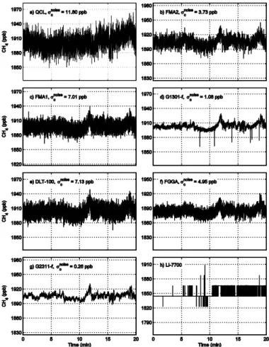
This is evident in the example fast-response time series shown in Fig. 5. For the two Picarro instruments the turbulent signal can easily be seen in the time series (high concentration during upward motion and close to ambient concentration during down-ward motion), while for the other instruments the signal in CH4 concentration is mixed with instrumental noise and is therefore not visible as clearly. All the other gas
analy-10
sers show much higher instrumental noise levels; FGGA had the smallest instrumental noise of the non-Picarro analysers, while QCL had the highest.
The instrumental noise of the FMA1 was highly variable during the experiment and affected by cell temperature: when the cell temperature of the FMA1 was between 27◦C and 29◦C, the instrumental noise was approximately 13.8 ppb and reached up to
15
20 ppb, whereas in other situations (cell temperature above 29◦C or below 27◦C) it was on average 6.8 ppb. The reason for this odd temperature dependence is unknown. The noise in the FMA2 data also responded to cell temperature, but not as strongly as for the FMA1 instrument. Instrumental noise from other analysers by Los Gatos Research did not show such strong temperature dependence.
20
The LGR analysers report also cavity ringdown (CRD) times which describe how long it takes for the laser signal to attenuate in the optical cavity. Roughly speaking the CRD time can be thought to represent cleanliness of the mirrors in the cavity: short CRD time corresponds to dirty mirrors and long CRD time to clean mirrors. For most of the LGR analysers the CRD times decreased significantly during the campaign due
25
BGD
11, 797–852, 2014Evaluating the performance of EC
CH4 analysers O. Peltola et al.
Title Page
Abstract Introduction
Conclusions References
Tables Figures
◭ ◮
◭ ◮
Back Close
Full Screen / Esc
Printer-friendly Version
Interactive Discussion
Discussion
P
a
per
|
D
iscussion
P
a
per
|
Discussion
P
a
per
|
Discuss
ion
P
a
per
|
still usable for flux calculations. For example for FMA1 the instrumental noise increased from 6.5 ppb to 7.8 ppb when the CRD time was above 10 µs or below 8 µs (only periods when cell temperature was above 29◦C or below 27◦C were considered).
The detection limits, shown in Fig. 4c, were approximately 2 nmol m−2s−1, except for the QCL and the FMA2, which had higher values (4 nmol m−2s−1). The flux detection
5
limit estimated with this method is mostly determined by the stochastic nature of turbu-lence during the 30 min periods selected. For the QCL the high noise level increased also the value of the detection limit, but the higher detection limit for FMA2 is not expli-cable in terms of white noise, since for instance FMA1 had more white noise but lower detection limit when compared to FMA2. Possibly, the FMA2 signal was contaminated
10
also with (structured) noise rather than just white noise, which contributed more to the detection limit than to the instrumental noise.
4.3 Flux corrections
4.3.1 Spectral corrections
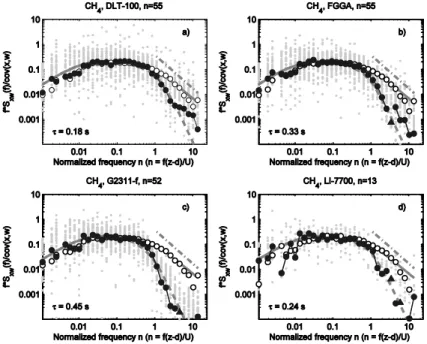
Ensemble-averaged methane cospectra are shown in Figs. 6 and 7, together with the
15
corresponding temperature cospectra. In the ideal case the methane cospectra would collapse onto the temperature cospectra and both would follow the model cospectrum, which is also shown for reference. However, all methane cospectra fell below the tem-perature cospectrum at the high frequency end.
As the flux is the integral of the cospectrum, it is clear that the contribution of the
20
high frequency fluctuations (small eddies) is underestimated and should be corrected. This is done with the method presented in Sect. 3.2; the response times used for the corrections are given in the figures. G2311-f had the slowest response time which was caused by instrument malfunction: although the instrument was set to measure at 10 Hz, it was effectively measuring at approximately 2.3 Hz, and the recorded 10 Hz
25
BGD
11, 797–852, 2014Evaluating the performance of EC
CH4 analysers O. Peltola et al.
Title Page
Abstract Introduction
Conclusions References
Tables Figures
◭ ◮
◭ ◮
Back Close
Full Screen / Esc
Printer-friendly Version
Interactive Discussion
Discussion
P
a
per
|
D
iscussion
P
a
per
|
Discussion
P
a
per
|
Discuss
ion
P
a
per
|
by a memory leak produced by some additional code designed specifically for this campaign and added to the instrument’s internal software (Gloria Jacobson, Picarro Inc., personal communication, 2013). Thus, if this is the case, other G2311-f analysers should not be affected.
The magnitudes of spectral corrections are presented in Fig. 8 as percentages of the
5
measured raw fluxes. At close to 40 %, the correction was largest for the G2311-f. This is not surprising since it had the slowest response time. For the other methane fluxes the correction ranged from 10 to 30 % of the originally measured flux.
4.3.2 Density and spectroscopic corrections
As a test, the CH4fluxes of the FGGA were calculated by applying the H2O corrections
10
point-by-point (Eq. 4) and comparing these values to half-hourly fluxes calculated using block-averaging and corrected using (Eq. 5). Linear fit to the data processed with the two methods has a slope of 1.000 and intercept of−0.001 nmol m−2s−1and RMSE and correlation coefficient (r) are 0.008 nmol m−2s−1and 1.000, respectively. The excellent agreement between the datasets confirms that the two correction methods are identical
15
and that the choice of correction method should not induce a systematic bias between the instruments, as long as the water vapour flux used in Eq. (5) is calculated with the same lag time as the CH4flux.
The magnitude of density and spectroscopic corrections are given in Fig. 8. The den-sity correction was on average approximately 10 % during the day and a few percents
20
at night when water vapour fluxes were small. Spectroscopic corrections were much smaller: a few percent during the day and less than a percent at night time. However, the LI-7700 is an exception: the density correction was on average 40 % during the day and−27 % at night. In addition, the spectroscopic correction was also larger (daytime 14 %, night time−13 %). The difference between the LI-7700 and the other gas
analy-25
BGD
11, 797–852, 2014Evaluating the performance of EC
CH4 analysers O. Peltola et al.
Title Page
Abstract Introduction
Conclusions References
Tables Figures
◭ ◮
◭ ◮
Back Close
Full Screen / Esc
Printer-friendly Version
Interactive Discussion
Discussion
P
a
per
|
D
iscussion
P
a
per
|
Discussion
P
a
per
|
Discuss
ion
P
a
per
|
To validate the density and spectroscopic corrections applied, the corrected CH4 fluxes were compared with the fully corrected G2311-f CH4 flux. This instrument does both corrections automatically during measurement using coefficients reported in Chen et al. (2010) and it has been shown that the automatic correction implemented in Picarro instruments performs well (e.g. Rella et al., 2013). Thus the fully corrected
5
G2311-f CH4 flux is a good reference for the other instruments and there should not be any residual H2O effect left in G2311-f fluxes. A linear correlation between the dif-ference in methane flux and the density correction term (FCHWPL
4 , second term on right
hand side in Eq. 5) was used to evaluate if the corrections were done properly (Fig. 9 shows an example using FGGA data). If the slope equals zero, the H2O corrections
10
were done correctly and the differences between CH4flux time series does not depend onFCHWPL
4 .
Values for the slope before and after applying the H2O corrections are given in Ta-ble 4. Before applying the H2O correction, the slopes differ from zero and the diff er-ence from zero is statistically significant. This was expected since the fluxes were still
15
affected by density and spectroscopic effects and the difference should be related to
FCHWPL
4 . If the slope is small before the H2O corrections is applied, it can be said that for
that setup the effect of H2O on CH4fluxes is small. This presumably can be explained by enhanced phase and amplitude shifts of H2O signal in that particular setup which diminish the effect of H2O on CH4flux measurements. This is the case for instance for
20
DLT-100 for which the slope was−0.181 before applying any H2O corrections.
For the QCL no density or spectroscopic corrections were applied, because the gas analyser was connected to a drier. In theory, the differences between G2311-f and QCL methane fluxes should not correlate withFCHWPL
4 , since both should be free from
any interference from H2O. This is supported by the small slope derived for the QCL of
25
BGD
11, 797–852, 2014Evaluating the performance of EC
CH4 analysers O. Peltola et al.
Title Page
Abstract Introduction
Conclusions References
Tables Figures
◭ ◮
◭ ◮
Back Close
Full Screen / Esc
Printer-friendly Version
Interactive Discussion
Discussion
P
a
per
|
D
iscussion
P
a
per
|
Discussion
P
a
per
|
Discuss
ion
P
a
per
|
not significantly different from zero; this suggests that the coefficients obtained from Hiller et al. (2012) were applicable to the FGGA used in this study. Only the slopes for DLT-100 and FMA1 remained statistically significantly different from zero, even af-ter correction. DLT-100 fluxes were over-corrected (the slope was positive afaf-ter H2O correction) and FMA1 fluxes were under-corrected (the slope was negative after H2O
5
corrections). Neither of these gas analysers measured H2O and thus external water vapour measurements were needed to correct their CH4fluxes. Assuming that the co-efficients obtained from Hiller et al. (2012) are applicable to the DLT-100 and FMA1 used in this study, the non-zero slopes suggest that the empirical method used to pa-rameterize the lag time difference between the H2O signal and other scalar signals
10
(Sect. 3.4.1) was not fully successful. Moreover, different attenuation and shape of the cross-covariance function may have contributed to the miscalculation of the H2O cor-rection (see Sect. 4.3.3 and Fig. 10). For the DLT-100 the value of the covariance of
w with H2O, w′χ ′
v, used in Eq. (5) appears to have been too high and for the FMA1 too small. In the case of the G1301-f, which did not measure H2O either, the method
15
seemed to overcorrect the data since the slope was positive (0.259), but the difference from zero was not statistically significant.
The above discussion deals with the systematic error in the H2O correction. Despite the fact that the correction is highly sensitive to the lag time, attenuation and the shape of the cross-covariance function, one might be tempted to use external H2O
measure-20
ments to correct CH4fluxes if the H2O obtained from the CH4analyser is noisy. Uncer-tainties inw′χ′
candw′χ ′
vcalculated with the data from FGGA were estimated based on Finkelstein and Sims (2001) and this uncertainty is assumed to be the total uncertainty ofw′χ′
v. By applying error propagation to Eq. (5) we can estimate how much the noise inw′χ′
vis affecting the precision of CH4fluxes when the density and spectroscopic
cor-25
rections are done. Relative uncertainty of FGGA CH4 fluxes is increased from 24.3 % to 24.4 % after applying the H2O corrections. If the uncertainty in w′χ′
BGD
11, 797–852, 2014Evaluating the performance of EC
CH4 analysers O. Peltola et al.
Title Page
Abstract Introduction
Conclusions References
Tables Figures
◭ ◮
◭ ◮
Back Close
Full Screen / Esc
Printer-friendly Version
Interactive Discussion
Discussion
P
a
per
|
D
iscussion
P
a
per
|
Discussion
P
a
per
|
Discuss
ion
P
a
per
|
said that use of noisy water vapour data in the H2O corrections does not compromise the precision of CH4 fluxes. Moreover if the CH4 analyser also measures H2O these measurements should be used to correct the methane data no matter how noisy the H2O signal is, rather than external water vapour data.
4.3.3 Correcting CH4fluxes without concurrent H2O measurements
5
Fig. 10 exemplifies the problem of using external H2O measurements. The cross-correlation between CH4(FGGA) and w, and between H2O (FGGA) andw both peak at different lag times even though the gases are measured with the same sampling line and instrument. The difference is caused by the sorption/desorption of H2O on the internal walls of the sampling tube and filters. The H2O cross-covariances shown in
10
these plots are normalized with the values that should be used in Eq. (5) for correcting FGGA CH4fluxes (blue dots in the plots). Thus, for instance, if in these situations the covariances between H2O (FGGA) andware maximized and then used in the H2O cor-rections, the corrections are overestimated by 132 % (left plot in Fig. 10) and 21 % (right plot in Fig. 10). Moreover, the two H2O cross-covariances (LI-7000 and FGGA) shown
15
in both plots have different degree of attenuation, the FGGA H2O cross-covariance being more attenuated, and the shape of the cross-covariance is affected by the tube effects. The FGGA H2O cross-covariance functions are wider and the peaks not as sharp as in the LI-7000 H2O cross-covariances. In order to successfully correct CH4 fluxes using H2O covariance measurements, all three effects (lag time, attenuation and
20
shape of the cross-covariance) induced on H2O by the sampling line must be properly taken into account. If the H2O is measured by the same instrument as the CH4, this is achieved by calculating the water vapour covariance with the same time-lag that is used for calculating the CH4 flux. If H2O is measured by an external instrument, the effects need to be estimated.
25
BGD
11, 797–852, 2014Evaluating the performance of EC
CH4 analysers O. Peltola et al.
Title Page
Abstract Introduction
Conclusions References
Tables Figures
◭ ◮
◭ ◮
Back Close
Full Screen / Esc
Printer-friendly Version
Interactive Discussion
Discussion
P
a
per
|
D
iscussion
P
a
per
|
Discussion
P
a
per
|
Discuss
ion
P
a
per
|
measurements. The LI-7000 H2O covariance used in Eq. (5) was modified with four different methods (see Fig. 10): the covariance between LI-7000 H2O andw was max-imized and then used in Eq. (5) (no revision), LI-7000 H2O cross-covariance maximum was adjusted to be the same as FGGA H2O cross-covariance maximum (Attenuation revised), LI-7000 H2O lag time was revised to match FGGA H2O lag time (Lag time
5
revised) and both, attenuation and lag time, are revised (Both revised). A compari-son between these four methods and the reference correction calculated using in-situ FGGA H2O measurements is shown in Fig. 11. With no revision applied to LI-7000 H2O data (i.e. the water vapour covariance is calculated from the LI-7000 data choosing the time lag that maximizes the covariance for that sensor), the correction is clearly
over-10
estimated, by approximately 2.85 nmol m−2s−1 (74 % overestimation), when LE was above 150 W m−2. If the attenuation is revised this error decreases to 1.07 nmol m−2s−1 (25 % overestimation), if the lag time is revised the error is 0.24 nmol m−2s−1 (5 % overestimation) and if both are revised the correction becomes underestimated by 0.88 nmol m−2s−1 (21 % underestimation). By revising both, attenuation and lag time,
15
the results were worse than just by altering the lag time. This stems from the fact that the shape of the H2O cross-covariance is also altered which was not accounted for here.
The fact that H2O corrections are highly sensitive to the lag time used in calcu-latingw′χ′
v result from the shape of cross-covariance betweenw and χv. The
cross-20
covariance betweenw and χvis an exponential function of the time lag between the time series and thus the error in the correction increases exponentially when error in the lag increases.
4.4 Agreement between flux estimates
After corrections have been applied as well as possible, all the instruments agreed
25
BGD
11, 797–852, 2014Evaluating the performance of EC
CH4 analysers O. Peltola et al.
Title Page
Abstract Introduction
Conclusions References
Tables Figures
◭ ◮
◭ ◮
Back Close
Full Screen / Esc
Printer-friendly Version
Interactive Discussion
Discussion
P
a
per
|
D
iscussion
P
a
per
|
Discussion
P
a
per
|
Discuss
ion
P
a
per
|
were acceptable, ranging from−6.835 (LI-7700) to 2.997 nmol m−2s−1(DLT-100). The values of the correlation coefficient were close to one, which implies that all flux results are highly correlated. The LI-7700 had the highest value of root mean square error (RMSE); this implies that it had the highest scatter in CH4 fluxes. This might be at least partly caused by the LI-7700 data logging problem and partly caused by the fact
5
that it is an open-path gas analyser and the open sampling cell was vulnerable to disturbances which might appear as high variation in the fluxes. Of the closed-path instruments FMA2, QCL and G1301-f gave the highest values for RMSE.
Despite the good agreement between the CH4fluxes shown in Table 5, there seems to have been a systematic bias between the different instruments which is revealed
10
by the cumulative sums shown in Fig. 12 (left plot). Most of the flux time series gave a value around 360 mg m−2 for the cumulative CH4emission during the 13 days long period shown in the plot, however three time series deviated most from this value: FMA1 and QCL derived about 330 mg m−2and the DLT-100 399 mg m−2for the cumu-lative sum.
15
Cumulative CH4 emissions from three gas analysers (G2311-f, FGGA and FMA2) agree best. For these three analysers the H2O corrections were done using internal H2O measurements and thus it can be assumed that the corrections were done accu-rately. Two out of the three time series which diverged most from the mean (DLT-100 and FMA1) were corrected with external H2O measurements, which suggests that the
20
differences in cumulative CH4 emissions could have been caused by the H2O correc-tions. To test this, the H2O corrections were adjusted so that the slopes in the column on the right in Table 4 became zero, meaning that a time series−kFCHWPL
4 , wherek is
the slope, was added to the fluxes. After the adjustment the difference between the G2311-f CH4flux and other CH4fluxes no longer depended onFCHWPL
4 . Cumulative CH4
25
BGD
11, 797–852, 2014Evaluating the performance of EC
CH4 analysers O. Peltola et al.
Title Page
Abstract Introduction
Conclusions References
Tables Figures
◭ ◮
◭ ◮
Back Close
Full Screen / Esc
Printer-friendly Version
Interactive Discussion
Discussion
P
a
per
|
D
iscussion
P
a
per
|
Discussion
P
a
per
|
Discuss
ion
P
a
per
|
Monthly values were calculated by computing mean values for the CH4fluxes during 12 to 25 June (same time period as in Fig. 12) and then multiplying the mean val-ues with the length of the month June (Fig. 13). Figure 13 shows the same pattern as Fig. 12: the DLT-100 initially gave higher fluxes and the FMA1 gave lower fluxes than all the analysers on average; however, the difference decreased if the H2O corrections
5
were set to match the G2311-f. For the DLT-100 the difference between fluxes calcu-lated with original and adjusted H2O correction on a monthly scale was approximately 0.1 g (CH4) m−2, which is 8 % of the monthly CH4 emission observed on average. These results highlight the importance of proper H2O corrections, especially for calcu-lating long term CH4balances. As the absolute value of the H2O corrections depends
10
on the magnitude of the latent heat flux, the corrections are significant in locations where latent heat fluxes are large and CH4fluxes are low.
The slightly smaller cumulative CH4 emissions observed with QCL, FMA2 and FMA1 than with the other three gas analysers cannot be explained by the use of two anemometers: the anemometer which was accompanying the three analysers
15
mentioned above (METEK2) gave on average 4 % larger value for turbulence inten-sity (σw/U) and 2 % larger value for sensible heat flux than the other anemometer (METEK1). This implies that the fluxes measured with METEK2 should not be under-estimated compared to fluxes measured with METEK1.
5 Discussion
20
All three previously published CH4flux inter-comparison studies (Detto et al., 2011; Pel-tola et al., 2013; Tuzson et al., 2010) showed relatively good correspondence between measured CH4fluxes. Detto et al. (2011) compared the performance of LI-7700 against two LGR analysers (FMA and FGGA) and they showed that minimum detectable flux was similar from all instruments and the fluxes from LI-7700 agreed with the
closed-25