Four-year (2006–2009) eddy covariance measurements of CO<sub>2</sub> flux over an urban area in Beijing

(1)

H. Z. Liu1, J. W. Feng1, L. J¨arvi2, and T. Vesala2

1_{LAPC, Institute of Atmospheric Physics, Chinese Academy of Sciences, Beijing 100029, China} 2_{Department of Physics, University of Helsinki, P.O. Box 48, 00014 University of Helsinki, Finland}

Correspondence to:H. Z. Liu (huizhil@mail.iap.ac.cn)

Received: 25 November 2011 – Published in Atmos. Chem. Phys. Discuss.: 16 March 2012 Revised: 22 August 2012 – Accepted: 22 August 2012 – Published: 3 September 2012

Abstract.Long-term measurements of carbon dioxide flux (Fc) and the latent and sensible heat fluxes were performed using the eddy covariance (EC) method in Beijing, China over a 4-yr period in 2006–2009. The EC setup was installed at a height of 47 m on the Beijing 325-m meteorological tower in the northwest part of the city. Latent heat flux dom-inated the energy exchange between the urban surface and the atmosphere in summer, while sensible heat flux was the main component in the spring. Winter and autumn were two transition periods of the turbulent fluxes. The source area of

Fcwas highly heterogeneous, which consisted of buildings, parks, and highways. It was of interest to study of the tempo-ral and spatial variability ofFcin this urban environment of a developing country. Both on diurnal and monthly scale, the urban surface acted as a net source for CO2and downward fluxes were only occasionally observed. The diurnal pattern ofFcshowed dependence on traffic and the typical two peak traffic patterns appeared in the diurnal cycle. AlsoFc was higher on weekdays than on weekends due to the higher traf-fic volumes on weekdays. On seasonal scale,Fcwas gener-ally higher in winter than during other seasons likely due to domestic heating during colder months. Total annual average CO2emissions from the neighborhood of the tower were es-timated to be 4.90 kg C m−2_yr−1_{over the 4-yr period. Total} vehicle population was the most important factor controlling the inter-annual variability ofFcin this urban area.

1 Introduction

The proportion of the world’s population living in urban ar-eas has incrar-eased over the past several decades. In China,

urbanization has rapidly increased following the reform and opening policy in effect since 1978. At the end of 2009, 46.6 % (about 622 million) of China’s inhabitants resided in urban environments and this fraction is further expected to increase in future (Pan and Niu, 2010). One of the most important impacts of urbanization on local and regional cli-mates is the emissions associated with the combustion of fossil fuels (primarily CO2) to the atmosphere and changes in land use (Kalnay and Cai, 2003). Urban areas emit 30– 40 % of all anthropogenic greenhouse gases, even though they currently cover only about 4 % of the world’s dry land surface (Satterthwaite, 2008). CO2is one of the most impor-tant greenhouse gases and a significant increase in CO2 con-centrations from 280 ppm in pre-industrial times to 387 ppm in 2009 is the probable cause of the mean air temperature in-crease of approximately 0.6 K observed during the last 100 years (IPCC AR4, 2007). However, knowledge of the mag-nitude and temporal variability of surface-atmosphere CO2 exchange in cities has been limited up until the recent years. There is a need to make continuous CO2exchange measure-ments over urban surfaces to provide useful information for CO2emission monitoring and to local policies and decision makers to make plans to reduce CO2emissions from anthro-pogenic sources.

(2)

7882 H. Z. Liu et al.: Four-year (2006–2009) eddy covariance measurements of CO2flux

consider the heterogeneity and variability of the emission sources (Velasco and Roth, 2010). Advances in instrumenta-tion, notably the eddy covariance (EC) technique, offer a tool to directly measure representative flux data from urban areas. The EC technique has been widely used to measure the net CO2exchange of various natural or agricultural ecosystems as part of the global flux network (Baldocchi et al., 2000; Baldocchi et al., 2001), but its application in urban areas re-mains less common. With a few exceptions (Crawford et al., 2011), existing, published long-term (>3 years) urban flux data sets are rare. Moreover, urban EC studies have mainly focused on cities in developed countries (e.g. Grimmond et al., 2002; Nemitz et al., 2002; Vogt et al., 2006; Coutts et al., 2007; Vesala et al. 2008; Matese et al., 2009; Bergeron and Strachan, 2011; Pawlak et al., 2011). The characteristics of urban CO2exchange in developing countries, where the de-gree of industrialization is relatively lower than that in devel-oped countries, are largely unknown, with the only reported measurements from Mexico City (Velasco et al., 2005) and Cairo (Burri et al., 2009).

Urban CO2exchange measured with the EC method repre-sent an integrated response from anthropogenic, biogenic and meteorological factors, and the distribution of their sources and sinks is highly heterogeneous (Vogt et al., 2006). How-ever, urban areas are consistently reported to be a net source for CO2on both daily and seasonal timescales with a strong dependence on the vegetation fraction and human activities (Grimmond et al., 2002; Grimmond et al., 2004; Velasco et al., 2005; Vogt et al., 2006; Coutts et al., 2007; Vesala et al., 2008; Matese et al., 2009; Helfter et al., 2011). Maximum emissions are typically observed to be consistent with the highest traffic volumes during rush hours (Coutts et al., 2007; Vesala et al., 2008). Previous studies have also showed large variations of CO2flux on seasonal timescales (Vesala et al. 2008; Bergeron and Strachan, 2011; Crawford et al., 2011; Pawlak et al., 2011). Besides traffic, fossil fuel burning for domestic heating can also cause high CO2 emission levels in winter (Matese et al., 2009; Bergeron and Strachan, 2011; Pawlak et al., 2011). In less dense urban areas with a signifi-cant fraction of vegetation, CO2flux is partly reduced by ur-ban vegetation in summer, but the effect is not typically sig-nificant enough to offset the emissions from anthropogenic sources (Grimmond et al., 2002; Coutts et al., 2007).

As part of its promise to stage a green Olympics in 2008, Beijing made great efforts to improve its air quality. An odd-even traffic restriction scheme was implemented to reduce traffic congestion on the roads for two months (from July 20 to September 20). On days when odd numbered license plates were allowed, vehicles with license plates ending in an even number were prohibited from operating. This regu-lation was expected to take 1.95 million vehicles (about 58 % of the total vehicles) off the roads (Mao, 2008). In addition, many factories both in and around Beijing were closed for the duration of the Games because they were not expected to meet the temporarily increased environmental standards.

Song and Wang (2012) analyzed the impact of the reduction of vehicles on CO2 flux during the Games, and found sig-nificant lower flux during this period. However, the analysis was restricted to a year. The differences of CO2flux between weekdays and weekends, and the annual variations of CO2 emission in long-term period are of interest.

This study shows the first long-term urban CO2flux (Fc) from Beijing megacity measured with the EC method. This article also contributes to the small number of studies on the net CO2exchange in developing countries. The objectives of this study are: (1) to quantify the magnitude ofFcin Beijing; (2) to examine the temporalFcpatterns at diurnal, seasonal, and annual time scales; (3) to examine the spatial variability ofFc in a complex urban environment; and (4) to examine the annual variations of total CO2emission.

2 Site description and instrumentation

2.1 The Beijing megacity

Beijing, the capital of China, is among the most developed cities in China. It is located in the northern part of the North China Plain and is surrounded by the Yanshan Mountains to the west, north, and east (about 50 km), whereas the small al-luvial plain of the Yongding River lies to its southeast (about 45 km). The city has a moderate continental climate with hot, humid summers due to the East Asian monsoon and winters that are generally cold and dry, reflecting the influence of the Siberian anticyclone. The total population in Beijing ex-ceeded 22 million at of the end of 2009, making it one of the largest cities in the world. The municipality’s area was estimated to be 16 800 km2and the population density 1309 people per km2in 2009. Caused by rapid urbanization, the in-crease in vehicle numbers in Beijing has been dramatic: the number of registered vehicles has increased from 2.9 million in 2006 to 4 million by the end of 2009.

2.2 Site description

(3)

Fig. 1.Satellite photograph of the area around the measurement site taken from Google Earth. Source areas were calculated using the footprint model by Korman and Meixner (2001) from all half-hour data in 2006–2009. The white contours represent the percentage of the accumulated flux footprint within the contour. The black dot indicates the location of the tower. The purple line is the Beijing-Tibet Expressway, and the yellow line is the Beitucheng Road. The Yuan Dynasty Pelices Park is adjacent to the tower in the west.

situated in the south and the north, and these areas are charac-terized by low vegetation cover. In order to assess the source area of the fluxes, an analytical footprint model proposed by Kormann and Meixner (2001) was applied for the study pe-riod. The roughness length data input into the model were derived from Li et al. (2003). Other variables required by the model were derived from EC data. The result showed that the distance of the 90 % footprint was approximately 2 km around the tower (Fig. 1). In order to roughly estimate the percentage of vegetated area around the tower, image pro-cessing tools (such as Adobe Photoshop) were employed to filter the green color from the satellite photographs, which were taken from Google Map, and then calculate the per-centage. The percentage of vegetated area within a radius of 2 km around the tower was approximately 15 %. Within a circle corresponding to 50 % of the footprints, the surround-ing area can be divided into four different “Local Climate

(4)

Fig. 2.Monthly precipitation for each study year separately and monthly air temperature for the whole measurement period measured at Caoyang weather station. The open and solid square points indicate minimum and maximum air temperature. The error bars indicate one standard deviation.

2.3 Instrumentation

The EC setup was installed at 47 m of the tower to contin-uously measure the exchange of CO2, heat, water, and mo-mentum. The measurement height is almost 3 times the mean displacement height (∼16.7 m) in the close surroundings (ex-cept in the SW sector), which ensured that measurements were taken in the inertial sublayer (Grimmond et al., 2002, 2006). The iron tower was designed as an open lattice struc-ture. The cross section of the tower was an equilateral tri-angle, with side lengths of 2.7 m. EC sensors were mounted on a 5-m horizontal boom pointing to the NE direction. The structure of the tower and the setup of the sensors were de-signed to minimize flow distortions from the tower. A three-dimensional sonic anemometer (CSAT3, Campbell Scien-tific Inc., Logan, Utah, USA) was used to directly measure horizontal and vertical wind velocity components and sonic temperature. An open-path infrared gas analyzer (IRGA, LI-7500, Licor Inc., Lincoln, NE, USA) was used to measure fluctuations of water vapor and CO2concentrations. Both in-struments were operated at a sampling frequency of 10 Hz. The IRGA was calibrated at an interval of six months us-ing a dew point generator and standard gases. In addition, air temperature and humidity at the same level were measured using a thermometer and a hygrometer (developed in Insti-tute of Atmospheric Physics). In addition, wind speed and direction were measured at 47 m using cup anemometers and vanes (developed by the Institute of Atmospheric Physics). The daily and monthly precipitation or air temperature data were obtained from the Caoyang weather station about 10 km southeast of the site.

3 Method

In this study we analyzed the EC data over four-year period from 2006 to 2009. Vertical fluxF is calculated as a covari-ance between the vertical velocitywand scalarsof interest according to the eddy covariance technique (Lee et al., 2004):

F ₌w′_s′ ₍₁₎

(5)

Fig. 3.Frequency histogram of atmospheric stability in 0.1 bins during the whole measurement period(a)and categorized by the time of day(b). Transition period was defined by two hours centered on sunrise/sunset. The stability conditions were divided into three categories: unstable (ζ <₋0.05), near neutral or weakly stable (₋0.05< ζ <0.2) and stable (ζ >0.2). The atmospheric stability is usually in the near neutral or weakly stable condition during the night.

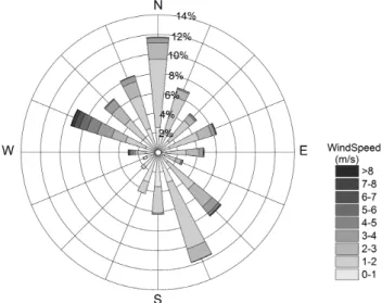
Fig. 4.The wind frequency distribution at 47 m derived from all available data from 2006 to 2009. The dominant wind direction is NW and SE.

approach developed for non-urban areas is problematic in ur-ban areas because the urur-ban boundary layer is not always sta-ble at night due to anthropogenic heat emissions, releases of storage heat to the boundary layer, and the heterogeneity of the urban canopy (Crawford et al., 2011). For our site, the frequency of the cases inu_∗ less than 0.2 m s−1_{at night is} 31.2 %, suggestingu_∗are large for most of the time at night in this urban environment. In fact, the atmospheric stratifi-cation is usually in the near neutral or weakly stable condi-tion during the night in Beijing (see seccondi-tion 4.1). Besides, an appropriateu_∗threshold is difficult to determine for its vari-ation and uncertainty. More errors may be introduced into the calculation of annual total flux when using this approach. Therefore, nou_∗filtering was applied in this study. The

stor-age term was omitted because the profile of CO2 concentra-tion in the canopy was not measured. On the other hand, it is considered that the storage term was minor in the calculation of annual total CO2emission (Crawford et al., 2011).

Data gaps originating from power failures, instrument cal-ibration errors, or sensor malfunctions accounted for 13.2 % during the four-year study period. Out-of-range data removal and spikes detection (outside 3 times of standard deviation from mean value) removed extra 3.1 % of data. Low-quality data caused by precipitation, dust, or other contamination on the sensor optics, which were indicated by the active gain control (AGC) values of the LI-7500, resulted in 6.9 % of eliminated data. Data that failed the stationary test caused another 6.1 % of the data gaps. Overall, the data coverage for the study period was approximately 70.2 %. Missing data were reconstructed using a gap-filling strategy as follows: (1) small gaps (<2 h) were replaced with linear interpola-tions; (2) medium gaps (<2 days) were rebuilt based on the mean diurnal variation (MDV) on adjacent days (Falge et al., 2001); and (3) large gaps (>2 days) were rebuilt using a mul-tiple imputation (MI) method following Hui et al. (2003). For

(6)

Fig. 5.The time series of sensible heat flux (H )(a), latent heat flux (λE)(b), carbon dioxide flux (Fc)(c)at 30 min interval, monthly Bowen ratio(d), and daily total precipitation(e)during the study period. The Bowen ratio was calculated using filled data when there were large gaps in a month.

Fig. 6.Average diurnal pattern of latent heat flux (λE)and sensible heat flux (H) in summer (JJA,a) and winter (DJF,b).

4 Results and discussion

4.1 Environmental conditions

General meteorological conditions during the study period are showed in Fig. 2. The annual total precipitation in Bei-jing for the four-year period was 473 mm in 2006, 452

(7)

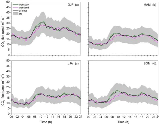
Fig. 7.Average diurnal pattern ofFcfor all days, weekdays and weekends separately in DJF(a), MAM(b), JJA(c)and SON(d)during the study period. The light gray shaded area represents one standard deviation from the mean for all days.

to 37.7◦_{C in June. The rainy season lasts from May to} Octo-ber, while the other time of the year is the dry season. Space heating is typically relevant from 15 November to 15 March in the next year in Beijing. But the period may be shifted to an earlier or later date (several days, commonly one or two weeks) according to the weather at the beginning of Novem-ber and that after 15 March. The atmospheric stability de-fined asζ₌(z−d) /L, wherezis the measurement height of the sonic anemometer andLis the Obukhov length, can be divided into three regimes: unstable (ζ <₋0.05), near neu-tral or weakly stable (−0.05< ζ <0.2) and stable (ζ >0.2). Observations in the four years showed that the number of un-stable cases was about 22.7 % more than the number of sta-ble cases (Fig. 3). The results also showed that the stability condition were unstable, or near neutral (or weakly stable) for most of the day in Beijing. The atmospheric stability in Beijing was different from that observed in London where the number of unstable cases at night was almost equal to the number during daytime (Wood et al., 2010). The stability conditions at night were mainly near neutral or weakly stable in Beijing. Also the fraction of strongly stable stratifications was relatively small at night in this urban area. The wind rose measured over the 4-yr period showed prevailing north-westerly and southeasterly winds (Fig. 4). Winds from the 270◦_–360◦_{sector occurred during 39.5 % of the study period,} whereas the 90◦_–180◦ _{sector accounted for 33.9 % of the}

study period. It should be noted that high wind speeds were recorded more frequently in the northwest sector, whereas the southwest sector experienced low wind speeds due to the tall buildings in this direction.

4.2 Time series of turbulence fluxes

Figure 5 shows the annual behavior of sensible heat flux (H), latent heat flux (λE), and carbon dioxide flux (Fc) at 30-min interval, and the daily precipitation measured at Caoyang weather station from 2006 to 2009. More than 80 % of the precipitation falls in the rainy season. Also monthly Bowen ratio calculated as a ratio between the sensible heat and latent heat fluxes is plotted. During the dry seasons,H is the dom-inant heat flux and reaches its maximum of 250–300 W m−2 in spring.λEis small (generally less than 100 W m−2₎ dur-ing the dry season due to the lack of precipitation and there-fore also evaporation (Fig. 5e). Bowen ratio reaches its max-imum 2–2.5 just in the beginning of the dry season whenλE

is below 100 W m−2_{. During the rainy season,} _λE _reaches its maximum of 250–350 W m−2_{in July or August, and the} Bowen ratio decreases to less than 0.5 (Fig. 5d). Positive (upward)Fcranging between 0–68.18 µmol m−2s−1are ob-served regardless of the season while the proportion of the negative flux is relatively small, with values generally from −34.09 to 0 µmol m−2_s−1_{(Fig. 5c). This indicates that CO}

(8)

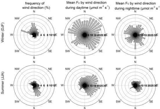
Fig. 8.Wind direction frequency, meanFcby wind direction during daytime (06:00 a.m.–10:00 p.m.) and nighttime (10:00 p.m.–06:00 a.m.) in different seasons. TheFcdata were calculated at 10◦intervals from all available non-gap-filled data during the study period.

emissions dominate the CO2 exchange between the urban surface and the atmosphere. Furthermore, the largest upward fluxes are observed in winter during the colder months when likely more traffic and domestic heating take place. The char-acteristic features ofFc variability on diurnal, seasonal and annual time scales analyzed below are based on this time se-ries.

4.3 Diurnal variation of energy fluxes

Average course ofλEwas found to be significantly changed between summer and winter (Fig. 6). MaximumλEat mid-day was observed to be 137.1 W m−2 _{in JJA, while it was} less than 20 W m−2 _{in DJF. The much higher}_λE _in sum-mer was caused by high evapotranspiration after the frequent rainfall events. MaximumH at midday was observed to be 67.8 W m−2_{in JJA, while it was 82.1 W m}−2_{in DJF. The} dif-ference of the average course ofHbetween summer and win-ter was not significant, with slightly higher maximum val-ues at midday in winter. The maximumH value at midday in winter was 14.33 W m−2_{higher than that in summer. The} results indicate that the climate makes a clear distinction be-tween the wet and dry season in Beijing city. The relationship between energy fluxes and climate in urban areas is beyond the scope of this paper and will not be discussed here.

4.4 Diurnal variation ofFc

For the diurnal Fc patterns, data was averaged over sons due to similarities in months (Fig. 7). During all

sea-sons the nocturnal fluxes are lower than in daytime when the diurnal variation is characterized by a distinct two peak pattern following the traffic rush hours. In winter, higherFcis measured over the mean diurnal course ranging from 15.9 to 31.82 µmol m−2_s−1_{, with an average value of} 18.86 µmol m−2_s−1_{. Also the morning peak is pronounced in} winter likely due to increased emissions from fossil fuel us-age during the colder months. Also the morning peak seemed to have two maxima: the first 26.59 µmol m−2_s−1_appeared at 08:00 and is related to intensive traffic flow. The second peak 30.45 µmol m−2_s−1_{at 11:00 is likely caused by the} hu-man activity and the more unstable stratification during day-time (Fig. 3b). On some occasions during the study period, the morning peak reached 68.18 µmol m−2_s−1_{. During other} seasons the net CO2fluxes are lower due to the increase in bi-ological processes and reduction in anthropogenic emissions. In summer, the mean diurnal course ranged from 8.86 to 18.86 µmol m−2_s−1_{, with an average of 12.73 µmol m}−2_s−1_. Unlike in winter, the morning peak ofFchas a single maxi-mum, as human activities began earlier during the warm sea-son and earlier sunrise. In all seasea-sons the evening peak is broad and maxima are observed between 18:00–20:00 indi-cating emissions from cooking and other household activ-ity after returning from work. In summer, the peak extended longer due to the longer day. The consistently positive values ofFc indicate that the source area is always a net source of CO2.

(9)

2007; Vesala et al. 2008; Bergeron and Strachan, 2011). The mean values ofFcmeasured at our site (18.86 µmol m−2s−1) in winter are lower than those in Montreal, Canada (∼20.0 µmol m−2s−1) (Bergeron and Strachan, 2011), Lon-don, England (∼33.32 µmol m−2s−1) (Helfter et al., 2011) and Firenze, Italy (∼25.68 µmol m−2s−1) (Matese et al., 2009). The mean values ofFcmeasured in the summer at our site were, by contrast, higher than those recorded in Mexico City in Mexico (∼9.32 µmol m−2s−1) (Velasco et al., 2005), Basel in Switzerland (∼12.5 µmol m−2s−1) (Vogt et al., 2006), and Melbourne in Australia (∼10.91 µmol m−2_s−1₎ (Coutts et al., 2007).

4.5 Spatial variation ofFc

The net CO2 exchange between the atmosphere and the ur-ban surface is a result of a combination of anthropogenic and biogenic processes. CO2sources and sinks are heterogeneous within the flux source area. The area of 50 % footprint in-cludes two busy roads in the north and east, the park in the west and the resident buildings in the north and south (Fig. 1). By analyzing the differences inFcvalues based on wind di-rection, it is possible to investigate the role of local sources in different surface cover areas (Fig. 8).

In winter, the dominant wind direction is northwest with 49 % of airflows coming from this direction. The highest

Fc values, i.e., about 28.41 µmol m−2s−1 during the day-time, are observed from the northeast portion of the study area, which corresponds to the sector with the heaviest traf-fic loads. During the night,Fc values in the east and north-east are substantially reduced due to the reduction of auto-mobile traffic. On cold winter nights, people usually do not go outside, and automobile traffic volumes are much lower than usually. The highestFcvalues are measured when winds blow from the northwest and south, where two dense residen-tial areas are situated.

In summer, the heavy automobile traffic on the express-way and the prevalent southeasterly winds contributed to the highest daytimeFcvalues (about 22.73 µmol m−2s−1). The measuredFcvalues in the west were much lower due to CO2 uptake by vegetation in the park. The photosynthetic pro-cesses by urban vegetation, even in such a small park, can play a role in the absorption of CO2. At night,Fc generally

collected from Caoyang weather station.

Year 2006 2007 2008 2009

TVP (million) 2.85 3.11 3.50 4.02

PPT (mm) 473 452 619 606

Ta(◦C) 24.74 25.21 25.12 26.26

drops below 9.10 µmol m−2_s−1_{, except in the southeast. The} higherFc values in the southeast are due to CO2emissions from the expressway in the prevalent wind direction. The re-sults reveal thatFc in urban areas is largely determined by the prevailing surface cover within the flux source area.

4.6 Annual variability of_Fc

Seasonal and annual variations of Fc are assessed by cal-culating average monthly Fc from the non-gap-filled half hourly dataset. As already shown by the diurnal behavior of

(10)

Fig. 9.Monthly averageFc calculated from non-gap-filled dataset and monthly average air temperature (Ta). The error bars indicate one standard deviation.

Table 3.Net annual carbon dioxide flux at urban sites around the world. The sites were selected for comparison based on two criteria: (1) annual CO2emission was estimated; (2) the environment around the site was highly urbanized. The Mexico site was analyzed by Velasco et al. (2005) using one month data, but the author rudely estimated the annual value, and this site was included in the comparison. The suburban sites were not included in the table, because they have highly vegetation cover and CO₂emissions were usually much lower than urban sites.

City Period Reference Annual Total (kg C m−2_yr−1₎

Mexico City, Mexico Apr 2003 Velasco et al. (2005) 3.49 Melbourne, Australia Feb 2004–Jun 2005 Coutts et al. (2007) 2.32 Essen, Germany Sep 2006–Oct 2007 Kordowski and Kuttler (2010) 1.64 London, UK Oct 2006–May 2008 Helfter et al. (2011) 9.67 Montreal, Canada Nov 2007–Oct 2009 Bergeron and Strachan (2011) 5.45 Ł’od´z, Poland Jul 2006–Aug 2008 Pawlak et al. (2011) 2.95 Beijing, China Jan 2006–Dec 2009 this study 4.90

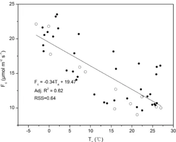
Fig. 10.The relationship between monthly averageFcand air tem-perature (Ta). The open circles represent the cases in 2008.

(11)

consistently positive CO2flux throughout the year indicates that the analyzed urban surface is a net source of CO2 to the atmosphere. Emissions from domestic heating are a con-siderable source of CO2in the winter. CO2sequestration by urban vegetation is not sufficient to offset emissions from local sources. (3) Spatial variation patterns of CO2flux are mainly determined by the prevailing surface cover within the flux source area. (4) The integrated annual net CO2exchange over the 4-yr period calculated from a gap-filledFcdataset is 4.90 kg C m−2_yr−1_{. This study shows an application of the} eddy covariance technique for long-term monitoring of CO2 flux in a densely built urban area. Total vehicle population was found to be the most important factor controlling the inter-annual variability ofFcin this urban area. The results presented here can provide valuable information for validat-ing emission inventories used for air quality and emission models.

Acknowledgements. This research was supported by the National Basic Research Program of China (973 Program, 2010CB951801), NSFC projects (41021004, 41030106). The authors thank Senior Engineer Li Aiguo (LAPC/IAP, CAS) for maintaining the ob-servation system. Thank also for anonymous reviewers’ valuable comments and suggestions.

Edited by: I. Trebs

References

Aubinet, M.: Eddy covariance CO2flux measurements in nocturnal conditions: An analysis of the problem, Ecol. Appl., 18, 1368– 1378, 2008.

Baldocchi, D., Finnigan, J., Wilson, K., Paw U, K. T., and Falge, E.: On measuring net ecosystem carbon exchange over tall veg-etation on complex terrain, Bound-Lay. Meteorol., 96, 257–291, 2000.

Baldocchi, D., Falge, E., Gu, L., Olson, R., Hollinger, D., Run-ning, S., Anthoni, P., Bernhofer, C., Davis, K., and Evans, R.: FLUXNET: A new tool to study the temporal and spatial variabil-ity of ecosystem–scale carbon dioxide, water vapor, and energy flux densities, B. Am. Meteorol. Soc., 82, 2415–2434, 2001. Bergeron, O. and Strachan, I. B.: CO2sources and sinks in urban

and suburban areas of a northern mid-latitude city, Atmos. Envi-ron. 45, 1564-1573, 2011.

Katul, G., Keronen, P., Kowalski, A., Lai, C. T., Law, B. E., Meyers, T., Moncrieff, J., Moors, E., Munger, J. W., Pilegaard, K., Rannik, U., Rebmann, C., Suyker, A., Tenhunen, J., Tu, K., Verma, S., Vesala, T., Wilson, K., and Wofsy, S.: Gap filling strategies for defensible annual sums of net ecosystem exchange, Agric. For. Meteorol., 107, 43–69, 2001.

Foken, T., G¨ockede, M., Mauder, M., Mahrt, L., Amiro, B., and Munger, W.: Post-field data quality control, in Handbook of Mi-crometeorology: A guide for surface flux measurement and anal-ysis, edited by X. Lee, W. Massman, and B. Law, Kluwer, Dor-drecht, The Netherlands, 181–208, 2004.

Grimmond, C. S. B.: Progress in measuring and observing the urban atmosphere, Theor. Appl. Climatol., 84, 3–22, 2006.

Grimmond, C. S. B., King, T., Cropley, F., Nowak, D., and Souch, C.: Local-scale fluxes of carbon dioxide in urban environments: methodological challenges and results from Chicago, Environ. Pollut., 116, S243–S254, 2002.

Grimmond, C. S. B., Salmond, J. A., Oke, T. R., Offerle, B., and Lemonsu, A.: Flux and turbulence measurements at a densely built-up site in Marseille: Heat, mass (water and car-bon dioxide), and momentum, J. Geophys. Res., 109, D24101, doi:10.1029/2004JD004936, 2004.

Helfter, C., Famulari, D., Phillips, G. J., Barlow, J. F., Wood, C. R., Grimmond, C. S. B., and Nemitz, E.: Controls of carbon dioxide concentrations and fluxes above central London, Atmos. Chem. Phys., 11, 1913–1928, doi:10.5194/acp-11-1913-2011, 2011. Hui, D., Wan S., Su, B., Katul, G., Monson, R., and Luo, Y.:

Gap-filling missing data in eddy covariance measurements using mul-tiple imputation (MI) for annual estimations, Agric. For. Meteo-rol., 121, 93–111, 2003.

Intergovernmental Panel on Climate Change: IPCC AR4 report, Contribution of working group I to the Fourth Assessment Report of the Intergovermental Panel on Climate Change, Cambridge University Press, Cambridge, UK and New York, NY, USA, 30– 31, 2007.

Kaimal, J. C. and Finnigan, J. J.: Atmospheric boundary layer flows: Their structure and measurement, Oxford University Press, New York, USA, 289 pp., 1994.

Kalnay, E. and Cai, M.: Impact of urbanization and land-use change on climate, Nature, 423, 528–531, 2003.

Kordowski, K. and Kuttler, W.: Carbon dioxide fluxes over an urban park area, Atmos. Environ., 44, 2722–2730, 2010.

(12)

Lee, X., Massman, W., and Law, B.: Handbook of micrometeorol-ogy: A guide for surface flux measurement and analysis, Kluwer, Dordrecht, The Netherlands, 250 pp., 2004.

Li, Q., Liu, H. Z., Hu, F, Hong, Z. X., and Li, A. G.: The determi-nation of the aero dynamical parameters over urban land surface (in Chinese), Clim. Environ. Res., 8, 443-450, 2003.

Mao, B. H.: Analysis on transport policies of post-olympic times of Beijing, J. Transp. Syst. Eng. Inform. Tech., 8, 138–145, 2008. Massman, W. J. and Lee, X.: Eddy covariance flux corrections

and uncertainties in long-term studies of carbon and energy ex-changes, Agric. For. Meteorol., 113, 121–144, 2002.

Matese, A., Gioli, B., Vaccari, F. P., Zaldei, A., and Miglietta, F.: Carbon dioxide emissions of the city center of Firenze, Italy: measurement, evaluation, and source partitioning, J. Appl. Me-teorol. Climatol., 48, 1940–1947, 2009.

Nemitz, E., Hargreaves, K. J., McDonald, A. G., Dorsey, J. R., and Fowler, D.: Micrometeorological measurements of the urban heat budget and CO2emissions on a city scale, Environ. Sci. Technol., 36, 3139–3146, 2002.

Pan, J. and Niu, F.: Annual report on urban development of china (in Chinese), Social Science Literature Publishing, Beijing, China, 92–100, 2010.

Pawlak, W., Fortuniak, K., and Siedlecki, M.: Carbon dioxide flux in the centre of Ł´od´z, Poland – analysis of a 2-year eddy covari-ance measurement data set, Int. J. Climatol., 31, 232–243, 2011. Satterthwaite, D.: Cities’ contribution to global warming: notes on the allocation of greenhouse gas emissions, Environ. Urbaniza-tion, 20, 539–549, 2008.

Schotanus, P., Nieuwstadt, F. T. M., and Bruin, H. A. R.: Temper-ature measurement with a sonic anemometer and its application to heat and moisture fluxes, Bound-Lay. Meteorol., 26, 81–93, 1983.

Song, T. and Wang Y. S.: Carbon dioxide fluxes from an urban area in Beijing, Atmos. Res., 106, 139–149, 2012.

Stewart, I. D.: Classifying urban climate field sites by “Local Cli-mate Zones”, Urban CliCli-mate News, 34, 8–11, available at: http: //www.urban-climate.org/IAUC034.pdf, 2009.

Velasco, E., Pressley, S., Allwine, E., Westberg, H., and Lamb, B.: Measurements of CO2fluxes from the Mexico City urban land-scape. Atmos. Environ. 39, 7433–7446, 2005.

Velasco, E. and Roth, M.: Cities as Net Sources of CO2: Review of atmospheric CO₂exchange in urban environments measured by eddy covariance technique, Geogr. Compass, 4, 1238–1259, 2010.

Vesala, T., J ¨ARvi, L., Launiainen, S., Sogachev, A., Rannik, ¨U., Mammarella, I., Siivola, E., Keronen, P., Rinne, J, Riikonen, A. N. U., and Nikinmaa, E.: Surface-atmosphere interactions over complex urban terrain in Helsinki, Finland, Tellus, 60B, 188– 199, 2008.

Vickers, D. and Mahrt, L.: Quality control and flux sampling prob-lems for tower and aircraft data, J. Atmos. Ocean. Technol., 14, 512–526, 1997.

Vogt, R., Christen, A., Rotach, M. W., Roth, M., and Satyanarayana, A. N. V.: Temporal dynamics of CO2 fluxes and profiles over a central European city, Theor. Appl. Climatol., 84, 117–126, 2006.

Webb, E. K., Pearman, G. I., and Leuning, R.: Correction of flux measurements for density effects due to heat and water vapour transfer, Q. J. Roy. Meteor. Soc., 106, 85–100, 1980.

Wood, C. R., Lacser, A., Barlow, J. F., Padhra, A., Belcher, S. E., Nemitz, E., Helfter, C., Famulari, D., and Grimmond, C. S. B.: Turbulent flow at 190 m height above London during 2006–2008: A climatology and the applicability of similarity theory, Bound-Lay. Meteorol., 137, 77–96, 2010.