Global distribution of the effective aerosol hygroscopicity parameter for CCN activation

(1)

www.atmos-chem-phys.net/10/5241/2010/ doi:10.5194/acp-10-5241-2010

Chemistry

and Physics

Global distribution of the effective aerosol hygroscopicity parameter

for CCN activation

K. J. Pringle1, H. Tost1, A. Pozzer1,2, U. P¨oschl1, and J. Lelieveld1,2

1_{Max Planck Institute for Chemistry, Mainz, Germany}

2_{The Cyprus Institute, Energy, Environment and Water Research Centre, Nicosia, Cyprus}

Received: 29 January 2010 – Published in Atmos. Chem. Phys. Discuss.: 8 March 2010 Revised: 1 June 2010 – Accepted: 9 June 2010 – Published: 15 June 2010

Abstract. In this study we use the ECHAM/MESSy Atmo-spheric Chemistry (EMAC) model to simulate global fields of the effective hygroscopicity parameterκ which approxi-mately describes the influence of chemical composition on the cloud condensation nucleus (CCN) activity of aerosol particles. The obtained global mean values ofκat the Earth’s surface are 0.27±0.21 for continental and 0.72±0.24 for ma-rine regions (arithmetic mean±standard deviation). These values are the internally mixedκcalculated across the Aitken and accumulation modes. The mean κ values are in good agreement with previous estimates based on observational data, but the model standard deviation for continental regions is higher.

Over the continents, the regional distribution appears fairly uniform, withκ values mostly in the range of 0.1–0.4. Lower values over large arid regions and regions of high or-ganic loading lead to reduced continental average values for Africa and South America (0.15–0.17) compared to the other continents (0.21–0.36). Marine regions show greater vari-ability withκvalues ranging from 0.9–1.0 in remote regions to 0.4–0.6 in continental outflow regions where the highly hygroscopic sea spray aerosol mixes with less hygroscopic continental aerosol. Marineκ values as low as 0.2–0.3 are simulated in the outflow from the Sahara desert.

At the top of the planetary boundary layer theκvalues can deviate substantially from those at the surface (up to 30%) – especially in marine and coastal regions. In moving from the surface to the height of the planetary boundary layer, the global average marineκ value reduces by 20%. Thus, sur-face observations may not always be representative for the altitudes where cloud formation mostly occurs.

In a pre-industrial model scenario, theκ values tend to be higher over marine regions and lower over the continents,

Correspondence to:K. J. Pringle (kirsty.pringle@mpic.de)

because the anthropogenic particulate matter is on average less hygroscopic than sea-spray but more hygroscopic than the natural continental background aerosol (dust and organic matter). In regions influenced by desert dust the particle hy-groscopicity has increased strongly as the mixing of air pol-lutants with mineral particles typically enhances theκvalues by a factor of 2–3 above the initial value of≈0.005.

1 Introduction

The ability of aerosol particles to take up water vapour influ-ences both their direct and indirect effects on climate. The aerosol water content controls the aerosol ambient radius – which in turn controls the ability of the particle to interact with solar radiation (direct effect). Also, it is the largest and most hydrophilic particles that are able to act as cloud condensation nuclei (CCN) and form cloud droplets (indirect aerosol effects).

The effective hygroscopicity parameterκ offers a simple way of describing the influence of chemical composition on the CCN activity of aerosol particles (Petters and Kreiden-weis, 2007). It can be used to calculate the CCN concen-tration, i.e., the number of particles within an aerosol pop-ulation that will activate at a specified water vapour super-saturation in K¨ohler model calculations without explicitly resolving the density, molecular mass and van’t Hoff fac-tor or osmotic coefficient and dissociation number of each chemical component. The applicability and usefulness ofκ

(2)

Based on a review of observational data, Andreae and Rosenfeld (2008) suggested that continental and marine aerosols on average tend to cluster into relatively narrow ranges of effective hygroscopicity (continentalκ= 0.3±0.1; marineκ= 0.7±0.2). Recent field studies are largely consis-tent with this view, but they show also systematic deviations for certain regions and conditions. For example, Gunthe et al. (2009) reported a characteristic value ofκ= 0.15 for pristine tropical rainforest aerosols in central Amazonia, which are largely composed on secondary organic matter.

Currently, the availability of observational data is not suf-ficient to obtain a clear picture of the global distribution and characteristic regional differences ofκ. In this study we use a general circulation model to calculate the global distribution ofκ. We outline and discuss horizontal and vertical distribu-tion patterns on regional and global scales, and we compare the model results with field measurement data. Moreover, we present the results of a pre-industrial model scenario and dis-cuss the effects of anthropogenic emissions. To our knowl-edge, such information has not been published before, and we hope that it will be useful for further experimental and theoretical studies of the hygroscopic properties and climate effects of atmospheric aerosols.

2 Methods

2.1 Model description

We used the ECHAM-MESSy Atmospheric Chemistry model (EMAC) to simulate global fields of aerosol loading and properties, including the hygroscopicity parameterκ as detailed below. EMAC is a combination of the ECHAM5 general circulation model (Roeckner et al., 2006) and the Modular Earth Submodel System (J¨ockel et al., 2005, 2006). For a full description of the EMAC model and evaluation see J¨ockel et al. (2005, 2006) or http://www.messy-interface.org. The model was run for a year with a spectral resolution of T42 degrees and with 19 levels in the vertical. The model was weakly nudged towards real meteorology using ECWMF analysis data for the year 2002.

Gas-phase chemistry is calculated in EMAC using the MECCA submodel (Sander et al., 2005). The wet deposition of gases and aerosols (both nucleation and impaction scav-enging) is treated within the SCAV submodel (Tost et al., 2006, 2007a), which describes scavenging due to convective and large-scale rain, snow and ice. Dry deposition is treated using the big leaf approach within the DRYDEP submodel (Ganzeveld and Lelieveld, 1995; Kerkweg et al., 2006a). Sedimentation is treated within the SEDI submodel (Kerk-weg et al., 2006a). Emission of gas and aerosols is treated by the ONLEM and OFFLEM routines (Kerkweg et al., 2006a). The other submodels used in this study are CONVECT (Tost et al., 2006), LNOX (Tost et al., 2007b), TNUDGE

(Kerk-weg et al., 2006b), as well as CLOUD, CVTRANS, JVAL, RAD4ALL, and TROPOP (J¨ockel et al., 2006).

The aerosol distribution is simulated using the GMXe model which simulates the distribution of sulfate, black car-bon, organic carcar-bon, nitrate, ammonium, dust and sea salt aerosol using 4 hydrophilic and 3 hydrophobic log-normal modes (in a similar approach to that of Vignati et al., 2004; Stier et al., 2005) in the following size ranges: nucle-ation (<5 nm radius), Aitken (5–50 nm), accumulation (50– 500 nm) and coarse (>500 nm). The 4 hydrophilic modes comprise a nucleation, Aitken, accumulation and coarse modes, the 3 hydrophobic modes are Aitken, accumulation and coarse modes. The aerosol composition within each mode is internally mixed, but the 7 modes are externally mixed with respect to each other, and notably the hydropho-bic and hydrophillic modes are chemically distinct.

Emission of black carbon (BC), organic carbon (OC), dust and sea salt aerosol are all taken from the AeroCom inven-tory (Dentener et al., 2006). To account for the presence of organic material and sulfate in the emitted sea spray aerosol, we assumed that 10% of accumulation mode sea spray con-sists of organic material and that 4% of the accumulation and coarse mode fluxes are marine sulfate (the rest was assumed to be NaCl). This approach is a simple approximation, but it is sufficient to avoid an overestimation of water uptake by sea spray aerosol. It resulted in aκ value of approximately 1.0 for freshly emitted sea spray aerosol, which is in good agreement with the experimental results of Niedermeier et al. (2008). More sophisticated treatments will be considered in future work.

The aerosol fields are compared to observations in Pringle et al. (2010), but to summarise, the model simulates global fields of the bulk aerosol species (SO4, DU, BC, OC and sea salt (SS)) within the range of the AeroCom global mod-els and with comparable proficiency to the ECHAM-HAM model (Stier et al., 2005). Nitrate ion concentrations have been compared to observations from EMEP (Europe) and CASTNET (N. America); annual mean modelled values compare to observations with a geometric mean ratio of 0.95 (EMEP) and 1.43 (CASTNET) with 77% (EMEP) and 50% (CASTNET) of modelled nitrate values within a factor of two of the observations. In the EMAC version applied in this study,κ was calculated as a diagnostic parameter that does not feedback on any other simulated parameter.

2.2 Calculation ofκ

The effective aerosol hygroscopicity parameterκis was cal-culated according to the simple mixing rule proposed by Pet-ters and Kreidenweis (2007);

κn= X

i

ǫi,nκi (1)

where ǫi,n and κi are the volume fraction and

(3)

n. The following parameter values were taken from Pet-ters and Kreidenweis (2007) (“CCN derived κ”): 0.61 for (NH4)2SO4, 0.67 for NH4NO3, 1.28 for NaCl, 0.90

for H2SO4, 0.88 for NaNO3, 0.91 for NaHSO4, 0.80 for

Na2SO4, 0.65 for (NH4)3H(SO4)2 For black carbon and

dust we tookκi= 0, and for organic carbon we tookκi= 0.1

(Wang et al., 2008; Gunthe et al., 2009; P¨oschl et al., 2009; Dusek et al., 2010; King et al., 2010). The assumed density (g cm−3) of each species is 1.70 for (NH4)2SO4,

1.72 for NH4NO3, 2.17 for NaCl, 1.84 for H2SO4, 2.26

for NaNO3, 1.48 for NaHSO4, 2.66 for Na2SO4, 1.78 for

(NH4)3H(SO4)2, 2.0 for black and organic carbon and 2.65

for dust.

According to Eq. (1), we calculatedκfor each of the seven aerosol modes of the model. For presentation and discussion we then calculate, from these mode dependentκ values, the volume weighted mean value of the Aitken and accumula-tion modes as this size range is most relevant for atmospheric CCN concentrations in the atmosphere and thus for compar-ison to field observations. For theκvalues presented in this work, we consider the volume fraction of each component in both the hydrophilic and hydrophobic modes, which corre-sponds to the bulk composition of fine particulate matter:

κ=Xκn·(Vn/Vt) (2)

whereκn is the calculatedκ of mode nandVn is the vol-ume of modenandVt is the aerosol volume summed across the relevant modes (Aitken hydrophilic, accumulation hy-drophilic, Aitken hydrophobic and accumulation hydropho-bic).

As demonstrated in several recent studies, this approach is well suited for approximate calculations of CCN num-ber concentrations from size distributions and bulk chemi-cal composition data of atmospheric aerosols (e.g., Wang, 2008; Bugiatioti, 2009; Chang, 2009; Gunthe, 2009; Shi-nozuka, 2009; Shantz, 2009; Ervens, 2009). However, by calculating a meanκ averaged between the hydrophobic and hydrophilic modes we loose information on the mixing state of the aerosol, which may lead to biases if these fields were to be used directly to calculate global fields of CCN in re-gions where there is a high degree of external mixing (e.g. some urban regions, see Cubison et al., 2008). Theκvalues presented are comparable to measurement-derivedκ values describing the total ensemble of CCN-active and -inactive aerosol particles (κt as presented and discussed by Gunthe

et al. (2009) and Rose et al. (2010)).

In the supplement we present an alternative data set considering only the hydrophilic Aitken and accumulation modes. Theκ values calculated this way are comparable to measurement-derivedκ values describing only the CCN-active particle fraction (κa as presented and discussed by

Rose et al. (2010) and Gunthe et al. (2009)). Depending on the proportion of hydrophobic and CCN-inactive particles, theseκ values can be significantly higher: the global

conti-nental averageκavalue is 0.07 (25%) larger than that calcu-lated considering both hydrophilic and hydrophobic modes, but this offset is fairly constant between regions (range of 0.07 to 0.10). Marineκvalues are less sensitive as there are fewer hydrophobic particles and thus κa is just 0.04 (5%)

larger.

For K¨ohler model calculations linkingκ to particle size and critical supersaturation for CCN activation, we used the surface tension of pure water (0.072 J m−2). This corre-sponds to the assumption that the effective hygroscopicity parameter accounts for solute effects on both water activity and surface tension (Petters and Kreidenweis, 2007; Gunthe et al., 2009; P¨oschl et al., 2009; Rose et al., 2010).

Throughout this text we present the calculated standard deviation of the simulatedκ values. Unless otherwise stated these standard deviations are calculated from data with a tem-poral resolution of five hours.

3 Results and discussion

3.1 Comparison with observations

The average effective hygroscopicity parameters calculated for continental and marine regions are

κcontinental=0.27±0.21 and κmarine=0.72±0.24,

respec-tively (surface level, Table 1). The mean value and standard deviation of κmarine are practically identical to

the observation-based estimate of Andreae and Rosenfeld (2008). For κcontinental the model-calculated mean value is

about 10% lower and the standard deviation is a factor of two higher than the estimate of Andreae and Rosenfeld (2008). Note, however, that the standard deviations calculated and reported in this study include both spatial and temporal variability unless noted otherwise (see Sect. 3.5.), whereas the observations reviewed by Andreae and Rosenfeld (2008) were mostly short-term measurements providing only lim-ited information about temporal variability. Considering that the two approaches used to estimate the average continental and marine κ values (Andreae and Rosenfeld, 2008, and ours) are completely different and independent, we find the overall agreement between the two studies quite good. In view of the limited observational database, we suggest that the model-derived standard deviation may be a more realistic estimator for the variability ofκ in continental aerosols.

(4)

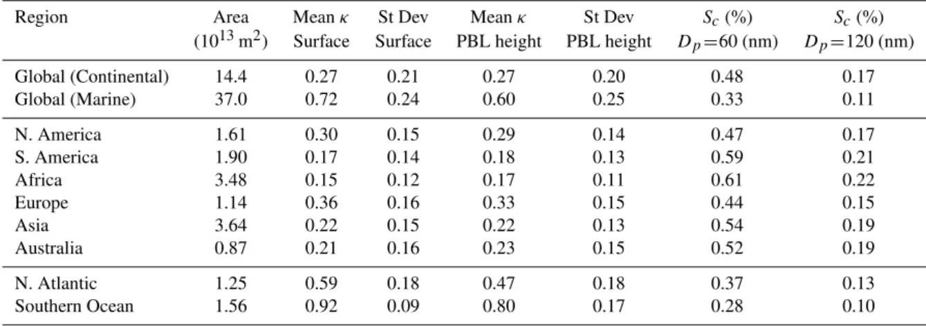
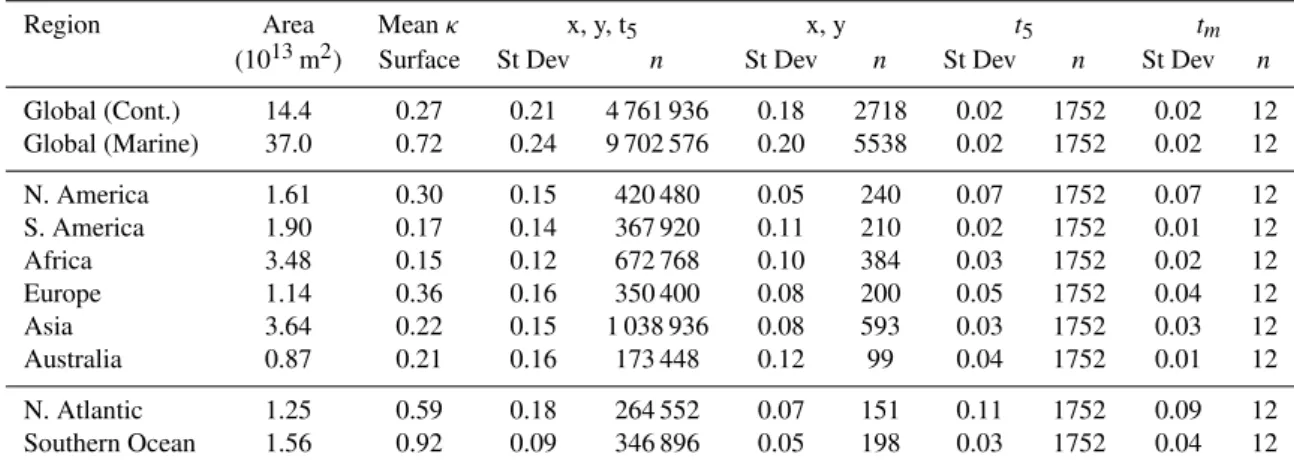
Table 1.Simulated global and regional annual meanκvalues (and standard deviation (St Dev)) at the surface and at the simulated PBL height under present day conditions. Standard deviation is calculated for the year from 5-hourly average data. Scis the critical supersaturation,

calculated using the regional meanκat PBL height. Area column gives total land area for land sites, and marine area for marine sites.

Region Area Meanκ St Dev Meanκ St Dev Sc(%) Sc(%)

(1013m2) Surface Surface PBL height PBL height Dp=60 (nm) Dp=120 (nm)

Global (Continental) 14.4 0.27 0.21 0.27 0.20 0.48 0.17

Global (Marine) 37.0 0.72 0.24 0.60 0.25 0.33 0.11

N. America 1.61 0.30 0.15 0.29 0.14 0.47 0.17

S. America 1.90 0.17 0.14 0.18 0.13 0.59 0.21

Africa 3.48 0.15 0.12 0.17 0.11 0.61 0.22

Europe 1.14 0.36 0.16 0.33 0.15 0.44 0.15

Asia 3.64 0.22 0.15 0.22 0.13 0.54 0.19

Australia 0.87 0.21 0.16 0.23 0.15 0.52 0.19

N. Atlantic 1.25 0.59 0.18 0.47 0.18 0.37 0.13

Southern Ocean 1.56 0.92 0.09 0.80 0.17 0.28 0.10

Table 2. Comparison between observed and modelledκvalues. Aκcalculated from reported aerosol soluble fraction, following Gunthe et al. (2009). Most measurement sites were surface campaigns, with the exception of Shinozuka et al. (2010) and Hudson (2007), which are flight data. For flight data an average altitude of approx. 1500 (m) was assumed.

Site Region Reference κobserved κmodel

1 Amazon Gunthe et al. (2009) 0.16±0.06 0.11

2 China Rose et al. (2010) 0.3 0.37

3 Mexico Shinozuka et al. (2010) 0.2–0.3 0.35

4 US West Coast Shinozuka et al. (2010) 0.18–0.47 0.23

5 Puerto Rico Allan et al. (2008) 0.6±0.2 0.70

6 Antigua Hudson (2007) 0.87±0.24 0.72

7 Amazon Vestin et al. (2007)A 0.10 0.08

8 Amazon Zhou et al. (2002)A 0.12 0.11

9 Tenerife Guibert et al. (2003)A 0.43 0.58

10 Germany (Feldberg) Dusek et al. (2006) 0.15–0.3 0.32

11 Germany (Munich) Kandler and Sh¨utz (2007)A 0.36 0.27

12 Eastern Mediterranean Bougiatioti et al. (2009) 0.24 0.44

13 Toronto Broekhuizen et al. (2006)A 0.15–0.3 0.31

14 Ontario Chang et al. (2010) 0.3 0.26

marineκthan that simulated by EMAC and that suggested by Andreae and Rosenfeld (2008). This is partly due to the fact that our marine value also includes data from the Southern Ocean whereκ values are large (>0.9, Fig. 1) whereas the marine data analysed by Wex et al. (2010) is often in conti-nental outflow regions where values of 0.5 to 0.7 are more common. Furthermore, it is conceivable that we underesti-mate the effects of the organic fraction in sea salt particles, which acts to reduceκ.

In Table 2 we compare effective hygroscopicity parame-ters derived from CCN measurements at various locations around the world to the values ofκcalculated by EMAC for the these regions (monthly mean modelled values for the time period of each campaign are used). Due to the large size of the global model grid boxes (approx. 250 km), the

compari-son with point observations is uncertain but necessary as no large-scale (e.g. satellite) measurements ofκexist. Note also that the model values are representative for the year 2002, whereas the observations were gathered over a range of dif-ferent years.

Nevertheless, the model results are in fair agreement with most observations. The deviations between modelled and ob-servedκvalues were≤0.05 for 10 out of the 14 measurement locations.

(5)

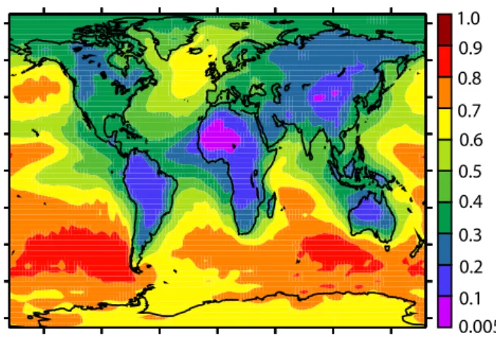
1.0 0.9 0.8 0.7 0.6 0.5 0.4 0.3 0.2 0.1 0.005

Fig. 1. Annual mean distribution ofκat the surface simulated by EMAC.

Overall, we find the agreement between model results and observations quite satisfactory when considering the uncer-tainties and complications involved in the comparison of a global model with sparse field measurement data.

3.2 Global distribution

Figure 1 shows the simulated annual mean global distribu-tion ofκ. This figure allows us to put the observedκvalues (discussed above) in the context of a wider geographical pat-tern.

The first thing to note is that in line with observations, the model simulates a distribution ofκthat has a strong land/sea contrast: the majority of continentalκ values lie in the range of 0.1 to 0.4, but marine regions have largerκ values, with most values>0.6. Inland continental regions strongly influ-enced by dust have the lowest simulatedκ, with values<0.1. No regions have an annual meanκof below 0.005.

The low resolution of the global model (T42) will under-estimate the horizontal variability ofκ, with values averaged over large gridboxes (approx. 250 km), but even if this effect is considered, the rate of change of κ across a geographic region is quite low, with regions of thousands of square kilo-metres showing quite constant annual mean values.

Coastal regions show the strongest horizontal gradient in

κand thus it is in these regions that the air mass history may significantly affect the water uptake potential of the aerosol and must therefore be considered in calculations.

One of the most striking aspects of Fig. 1 is the clear influ-ence of the continental regions on the marineκ values. Ma-rine regions downwind of continental outflow regions have a reducedκvalue, with some values as low as 0.2 (due to dust outflow from N. Africa). Outflow of anthropogenic pollution also influencesκ; for example in the Gulf of Mexico theκ

value is 0.4, clearly reduced from the “unpolluted” marineκ

values of>0.8. This effect extends over large parts of the

1.0 0.9 0.8 0.7 0.6 0.5 0.4 0.3 0.2 0.1 0.005

Fig. 2.Annual mean distribution ofκat the altitude of the planetary boundary layer.

ocean where the continental influence is large and is partic-ularly important where wind speeds are relatively low (and thus sea spray concentrations are quite small).

As the water uptake ability of the aerosol is important for cloud droplet formation, which occurs above the surface layer, it is also interesting to consider the distribution ofκ

at higher altitudes. Figure 2 showsκ at the simulated plan-etary boundary layer (PBL) height. We choose to extractκ

at the modelled PBL height, as it is a region of active cloud formation and therefore an altitude relevant for consideration of CCN and activation. In EMAC, the PBL height is calcu-lated using the TROPOP submodel (following the method of Holtslag et al., 1990; Holtslag and Boville, 1993) and can vary from 23 to 7291 m (the latter in mountainous regions), with an average value of 482 m above sea level.

At PBL height (as at the surface) there is a clear land/sea contrast, with low values (0.1–0.3) in S. America, parts of Africa and central Asia. Marine values are significantly lower above the surface layer; values>0.9 do not occur and the global mean marine κ value is reduced to 0.60 (from 0.72), reflecting the more aged nature of the aerosol distribu-tion and the reduced influence of sea salt. At the PBL height, the simulated annual meanκvalue is uniform over quite large geographical areas, although some coastal regions still show a strong horizontal gradient.

3.3 Vertical profiles

(6)

A

ltitude (hP

a)

200

400

600

800

1000

A

ltitude (hP

a)

200

400

600

800

1000

A

ltitude (hP

a)

200

400

600

800

1000

A

ltitude (hP

a)

200

400

600

800

1000

0.0 0.1 0.2 0.3 0.4 0.5 0.6 Kappa

0.0 0.2 0.4 0.6 0.8 1.0

Kappa

0.0 0.2 0.4 0.6 0.8 1.0

Kappa

a)

b)

c)

d)

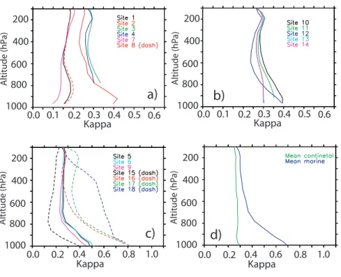
Fig. 3. Vertical distribution ofκat the sites shown in Fig. 4. Plots(a)and(b)show continental sites plot(c)shows continental sites with strong marine influence (solid line) and marine sites (dash) and plot(d)shows the vertical profile of the global mean of all continental and all marine regions. Note x-axis changes between plots.

1, 7,8

5,6 2

12 10,11 13,14

4

3 9

15 16

17

18

Fig. 4. Summary of the regions used in the consideration of re-gional values (large dashed boxes) and the approximate location of the field observation sites (over-plotted circles and squares). Stars represent additional regions taken for vertical profile plots.

marine regions are also shown. In this way we can see how representative surfaceκ values are for higher altitudes.

The variation ofκ with altitude of the single sites is com-plex. Amazonian sites (1, 7, 8) show an increase inκ with altitude caused by the hydrophobic BC particles ageing and become more hydrophilic at higher altitudes (up to 800 hPa, after whichκ decreases). The continentally influenced ma-rine sites (5, 6, 15, 16, and 17) all show a decrease inκ with altitude up to approximately 800 hPa (at which altitudeκcan be>30% smaller than at the surface). Although the S. Ocean site (18) shows an initial decline inκthe rate of decrease in

κwith altitude is lower than the other marine sites as the in-fluence of other (non-sea salt) aerosol types is smaller in this region. The marine sites show quite varied κ values even at high altitude. For example, theκ of Site 15, which is in the Saharan outflow region is still significantly below that of marineκvalues in less dusty regions. Although this is an ex-treme case (as few marine regions are so strongly influenced by continental aerosol) it is worth noting as at approximately 800 hPa theκof Site 15 is<0.2, which is far from the “typi-cal” marine value.

(7)

Jan _Feb M

ar Apr Ma_y Jul Sep O_ct No

v

D

ec

A

ug

Jun Jan _Feb M

v

D

ec

A

ug

Jun

Jan _Feb M

v

D

ec

A

ug

Jun Jan _Feb M

v

D

ec

A

ug

Jun

0.6

0.5

0.4

0.3

0.2

0.1

0.0

K

appa

0.6

0.5

0.4

0.3

0.2

0.1

0.0

K

appa

1.0

0.8

0.6

0.4

0.2

0.0

K

appa

1.0

0.8

0.6

0.4

0.2

0.0

K

appa

a)

b)

c)

d)

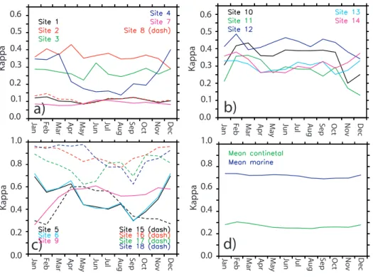
Fig. 5. Annual cycle of monthly meanκat the surface at sites shown in Fig. 4. Plots(a)and(b)show continental sites plot(c)shows continental sites with strong marine influence (solid line) and marine sites (dash) and plot(d)shows the annual cycle of the global mean of all continental and all marine regions. Note y-axis changes between plots.

Panel d shows the vertical variation ofκ averaged over all continental and all marine sites. The different vertical profiles of the continental sites tend to counteract each other, leading to a distribution that is almost constant with height. The mean marine profile, however, shows a strong decrease with height, with values reducing from 0.7 at the surface to 0.4 at 700 hPa.

3.4 Annual cycle

Many aerosol sources have a seasonal cycle and, often as a result of this, the chemical composition of the aerosol can change throughout the year, which can potentially affectκ. As most κ measurements are taken from field campaigns lasting a few weeks, it is worth examining howκ changes throughout the year to see how representative short term measurements are. Figure 5 shows the seasonal cycle ofκ

at each of the measurement sites considered previously (see Fig. 4).

The seasonal cycle ofκ is complex: all sites show some variation with month, although there is little consistency in the shape of the cycle. In Puerto Rico and Antigua (5 and 6),κ is>0.5 in the northern hemisphere winter and reaches a minimum of 0.3 in September. The mid Atlantic site (15) hasκ at a maximum in April and a minimum in winter.

Overall, at particular sites, the seasonal variation inκ can be strong, but the cycle varies so significantly between sites that it is difficult to draw a general trend. In many sitesκ

varies by±20% through the season, thus care must be taken when extrapolating from short term measurements to annual mean values. The global mean continental and marine κ

shows almost no seasonal cycle because the different cycles of the different locations cancel each other out.

3.5 Regional distributions

3.5.1 Continental

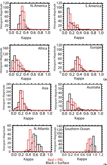
To examine the variability of κ within a region in more detail Fig. 6 shows histograms of the frequency of occur-rence of particularκvalues in 6 different continental regions: N. America, S. America, Africa, Europe, Asia and Australia (See Fig. 4) at both the surface (black line) and at PBL height (red line). The values taken for this analysis are annual mean values. In addition, Table 1 shows the average annual mean

κfor each region.

The frequency distribution ofκ on a continental scale is dependent on the region considered: S. America has very low

(8)

0.0 0.2 0.4 0.6 0.8 1.0

0.0 0.2 0.4 0.6 0.8 1.0 0.0 0.2 0.4 0.6 0.8 1.0

0.0 0.2 0.4 0.6 0.8 1.0

120 100 80 60 40 20 0 Hist o gr am M agnitude Kappa 120 100 80 60 40 20 0 Hist o gr am M agnitude Kappa Kappa Kappa 120 100 80 60 40 20 0 Hist o gr am M agnitude 160 120 80 40 0 Hist o gr am M agnitude

N. America S. America

Africa Europe

(a)

0.0 0.2 0.4 0.6 0.8 1.0

Hist o gr am M agnitude Kappa Asia 280 240 200 180 120 80 40 0 60 50 40 30 20 10 0 Hist o gr am M agnitude

0.0 0.2 0.4 0.6 0.8 1.0 Kappa 60 50 40 30 20 10 0 Hist o gr am M agnitude

0.0 0.2 0.4 0.6 0.8 1.0 Kappa

0.0 0.2 0.4 0.6 0.8 1.0 1.2 Kappa Australia Southern Ocean 140 120 80 60 40 20 0 100 Hist o gr am M agnitude

Black = SurfaceRed = PBL N. Atlantic

(b)

Fig. 6. Histogram of the occurrence of particular κvalues in the regions shown by the dotted boxes in Fig. 4. Histogram magnitude shows the total number of occurrences of eachκvalue calculated using a field of annual meanκvalues.

spread with just a small number of grid-boxes with larger values (these are generally boxes near the coast).

In Europe and N. Americaκ is larger (most values be-tween 0.2–0.4) and the distribution is broader. This surface distribution of κ in Asia is most frequently 0.2, but there are also much lower values<0.1 from biomass burning and high values from the largely anthropogenic sulfate and nitrate aerosol.

The distribution ofκ at PBL height is similar to the sur-face distribution, but in continental sites there is a general shift to largerκ values at altitude as the aerosol at altitude is generally more aged and thus the very lowκ values due to fresh dust and BC occur less frequently. In Europe the surfaceκ is quite similar to theκ aloft, but in N. America the frequency distribution of κ is quite different above the

Fig. 7. The relationship between particle diameter and critical su-persaturations plotted as done by Petters and Kreidenweis (2007), but with the lines corresponding to the simulated regional mean PBLκvalues highlighted.

surface layer. Thus, in this region, the dependence ofκ on altitude is important on a regional as well as a site specific scale.

3.5.2 Marine

Also shown in Fig. 6 is the distribution ofκ in two marine regions: the N. Atlantic and a remote section of the Southern Ocean. These regions were chosen to illustrate the potential range of marineκ values as the Southern Ocean region is very far from continental influences and the N. Atlantic is very strongly influenced by continental outflow of pollutants and dust.

(9)

0.25

0.2

0.15

0.1

0.05

-0.05

-0.1

-0.15

-0.2

-0.25

a) Absolute difference at surface

0.25

0.2

0.15

0.1

0.05

-0.05

-0.1

-0.15

-0.2

-0.25

b) Absolute difference at PBL top

300 200 100 50 40 30 20 10 -10 -20 -30 -40 -50 -100 -200 -300

d) Percentage difference at PBL top c) Percentage difference at surface

300 200 100 50 40 30 20 10 -10 -20 -30 -40 -50 -100 -200 -300

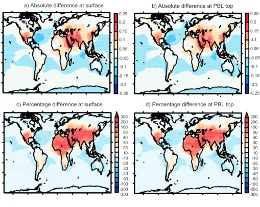
Fig. 8. Annual mean absolute difference inκ arising from present day emissions compared to a pre-industrial scenario (κpresent −

κpreindustrial) at(a)surface and(b)PBL height. Panels(c)and(d)show the percentage change due to present day emissions.

Over the N. Atlanticκ is more variable, with no one value dominating. The aerosol in this region is a much more com-plex mix of species, with differentκ values. The difference in the average κ value between these two marine regions is larger than the difference found between the various re-gional mean continental values (at surface: κS Ocean=0.92,

κN Atlantic=0.59). In line with the vertical profiles in Fig. 3,

the marine regions show a decrease inκ aloft as sea spray aerosol becomes a less dominant fraction of the aerosol mass. 3.5.3 Regional vs. temporal variability

Table 1 shows the average annual meanκ for each region and the standard deviation within the region. This calcula-tion of standard deviacalcula-tion uses 5 hourly averageκvalues for each grid box, and thus shows the deviation due to both the temporal variability and the variability within the region. In Sect. 3.4, it was shown that at point locations κ can vary throughout the season, but the implications for this on the larger scale are unclear. To elucidate this, Table 3 shows the standard deviation ofκ for each of the regions calculated in four different ways:

1. x,y,t5: Allows variation in area and time (five hourly

mean data, as used as default in this text).

2. x,y: Allows variation in area but annual averageκ val-ues are used.

3. t5: Allows for variation in time (using 5 hourly mean

data) but regional averageκvalues are used.

4. tm: Allows for variation in time (using monthly mean data) but regional averageκvalues are used.

In most regions the standard deviation ofκ due to time variability is small compared to the deviation due to vari-ability within the region implying that if a choice has to be made, it is better to focus analysis and measurements on the regional (rather than temporal) distribution ofκ. N. Amer-ica, however, has a more pronounced seasonal cycle than the other regions – κ values range from 0.4 to 0.2 with a minimum in June and July. A similar cycle is found in the N. Atlantic. In these regions the standard deviation due to variations in time (t5) is larger than that in space (x, y), for

(10)

Table 3.Standard deviation (St Dev) ofκvalues calculated considering variation in i) all dimensions (x, y, t5=area and time (t5=5 hourly

time intervals)), ii) area only (x, y), iii) time only (t5=5 hourly time intervals) and iv) time only (tm=monthly mean values used). For each

standard deviation value the adjacent column (to the right) shows the number of data points used in the calculation (n).

Region Area Meanκ x, y, t₅ x, y t5 tm

(1013m2) Surface St Dev n St Dev n St Dev n St Dev n

Global (Cont.) 14.4 0.27 0.21 4 761 936 0.18 2718 0.02 1752 0.02 12

Global (Marine) 37.0 0.72 0.24 9 702 576 0.20 5538 0.02 1752 0.02 12

N. America 1.61 0.30 0.15 420 480 0.05 240 0.07 1752 0.07 12

S. America 1.90 0.17 0.14 367 920 0.11 210 0.02 1752 0.01 12

Africa 3.48 0.15 0.12 672 768 0.10 384 0.03 1752 0.02 12

Europe 1.14 0.36 0.16 350 400 0.08 200 0.05 1752 0.04 12

Asia 3.64 0.22 0.15 1 038 936 0.08 593 0.03 1752 0.03 12

Australia 0.87 0.21 0.16 173 448 0.12 99 0.04 1752 0.01 12

N. Atlantic 1.25 0.59 0.18 264 552 0.07 151 0.11 1752 0.09 12

Southern Ocean 1.56 0.92 0.09 346 896 0.05 198 0.03 1752 0.04 12

This analysis implies that longer term measurement cam-paigns are particularly required to characteriseκin N. Amer-ica, N. Atlantic and Europe, although every region shows some variation due to the annual cycle. In general, regions that experience a strong annual cycle (i.e. the midlatitudes) will clearly experience the strongest temporal variability in aerosol composition (and κ) and thus long term measure-ments would be advantageous.

The final section of Table 3 shows the St Dev due to time, calculated using monthly mean values. In the regions which have high St Dev due to time (N. America, N. Atlantic), the calculated St Dev is not sensitive to the use of monthly mean rather than 5 hourly data – implying that the deviation comes from seasonal (not short term) variations. In other regions, using monthly mean data results in a smaller St Dev (values reduced by 30 to 60%). This happens because in regions with little seasonal cycle, short term variations are relatively more important for temporal variability. Overall in these regions, however, the deviations due to temporal variability are small compared to the St Dev due to changes inκacross the region (x,y).

3.6 Effect of regional meanκon critical

supersaturation required for CCN activation

So far, this paper has focused on the distribution of κ

throughout the globe. Theκvalue of an aerosol particle is of interest mainly because it can give information on the ability of a particle to activate during cloud formation. If variations inκhave a sufficiently small effect on the activation ability of the aerosol they can be neglected in activation calculations, conversely ifκ varies such that the critical supersaturation (Sc) required to activate a particle is significantly affected

then the particle composition (andκ value) must be consid-ered in detail.

Reutter et al. (2009) examined the sensitivity of cloud droplet number (CDN) concentrations toκ (0.05 to 0.6) for a typical biomass burning aerosol size distribution (assum-ing a s(assum-ingle lognormal mode) us(assum-ing a cloud parcel model. They found the value ofκ to be important at very low values (<0.05) and at larger values (κ>0.3) if the cloud regime sim-ulated was updraft-limited. In these cases a 50% change in the magnitude ofκ could change CDN by≥10%. Although this study was focused on one “typical” size distribution it indicates that changes inκcan significantly affect CDN, but the sensitivity depends on bothκ and the cloud regime.

In EMAC, we cannot capture the complex microphysics of a cloud parcel model, thus to place the different simulated regional meanκ values in the context of aerosol activation, Fig. 7 shows the relationship between particle diameter and

Scin the form shown by Petters and Kreidenweis (2007), but

with theκ lines corresponding to the meanκof the different regions (at PBL height) highlighted. Table 1 also shows the

Screquired to activate a particle of 60 and 120 nm diameter

in each of the different regions.

The Sc required for activation shows some variation

be-tween regions, for example to activate a particle of diame-ter 60 nm requires a supersaturation of 0.28% (in S. Ocean), 0.37% (N. Atlantic), 0.44% (Europe), 0.53% (Asia and Aus-tralia) and 0.6 (S. America and Africa). Similarly, to activate a 120 nm diameter particle requires a supersaturation of just 0.10% (in the S. Ocean), 0.13% (N. Atlantic) and 0.15% (Eu-rope), 0.19% (Asia and Australia) and 0.21% (in S. America and Africa). These regional differences can be significant in the formation of stratiform clouds which typically takes place at low supersaturations.

Nevertheless the variation of the annual meanκ between continental regions is small enough that the effect onSc(and

(11)

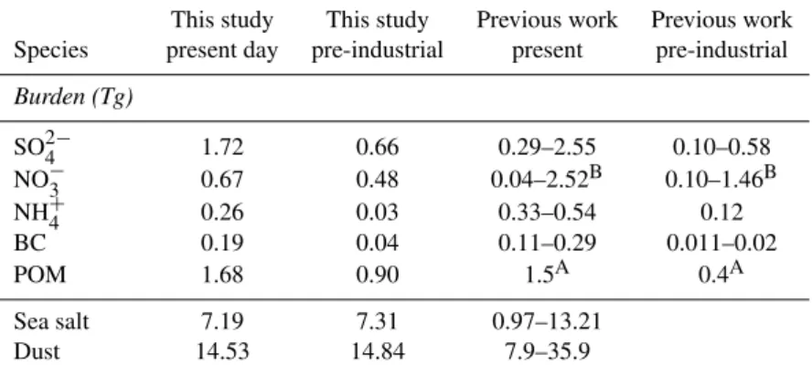
Table 4.Simulated aerosol burden in present day and pre-industrial conditions. Dust and sea salt emissions are identical in the present day and pre-industrial simulation. The review of previous works is taken from Tsigaridis et al. (2006), except for: AStier et al. (2005) andB Bauer et al. (2007). POM = Particulate organic matter, BC = black carbon. All units are Tg.

This study This study Previous work Previous work Species present day pre-industrial present pre-industrial

Burden (Tg)

SO2₄− 1.72 0.66 0.29–2.55 0.10–0.58

NO−₃ 0.67 0.48 0.04–2.52B 0.10–1.46B

NH+₄ 0.26 0.03 0.33–0.54 0.12

BC 0.19 0.04 0.11–0.29 0.011–0.02

POM 1.68 0.90 1.5A 0.4A

Sea salt 7.19 7.31 0.97–13.21

Dust 14.53 14.84 7.9–35.9

the global continental average to activate. Aerosols over the N. Atlantic and Southern Oceans require critical supersatura-tions that are, respectively, +13% and−15% different from the global mean marineScvalue to activate. In terms of the

absolute change inSc, this effect is more important for small

particles, as large particles activate at such low critical super-saturations that variations inκare less important.

Thus, although particle size is the dominant factor in aerosol activation, we show that there are small but sys-tematic differences in the mean water uptake ability of the aerosol between regions, which can affect activation. The result of this is that one can reasonably expect two aerosol distributions with the same number concentration and size distribution to form different concentrations of cloud con-densation nuclei (and cloud droplet number concentrations) if they originate from e.g. Asia rather than N. America or the N. Atlantic rather than the Southern Ocean. The use of globally uniformκ values would be unable to capture this subtlety.

3.7 Present vs. pre-industrial conditions: the influence of anthropogenic emissions

Human activities such as energy production, biomass burn-ing and transport are known to increase both the number and mass of aerosol particles in the atmosphere, with con-sequences for the radiative balance of the planet. However, in addition to changing the amount of aerosol in the atmo-sphere, anthropogenic emissions can also change the com-position of the atmospheric aerosol, which could affect the CCN formation ability of the aerosol.

To investigate the change inκas a result of human activi-ties, a second simulation was preformed in which emissions representative of pre-industrial conditions were used. Pre-industrial emissions of BC and OC provided by AeroCom are used (Dentener et al., 2006) and pre-industrial gas emis-sions are from the EDGAR-HYDE inventory (Van Aardenne

et al., 2001). Pre-industrial levels of CO2, N2O and CH4

are nudged (using the TNUDGE submodel) to values created using a previous long-term EMAC simulation (EVAL ver-sion 2.3, CO2: 284.7×10−6, CH4: 791.60×10−9and N2O:

275.68×10−9mol mol−1). For the pre-industrial simulation we use the same nudged meteorology as the present day run and no feedbacks of the aerosol or chemistry on radiation (and thus meteorology) are considered. Emission of dust and sea salt aerosol are also held constant. Nevertheless, the bur-den of these species may change as the degree and extent of mixing between hydrophobic and hydrophilic compounds can influence the aerosol scavenging efficiency by clouds and precipitation. A summary of the aerosol burdens for both simulations is given in Table 4.

Figure 8 shows the change inκ at both the surface and PBL height between the two simulations. Comparing the present with the pre-industrial scenario, many marineκ val-ues are reduced by 0.05 (or 10%). Over the continents, how-ever, present dayκ values are larger, particularly in Africa, N. America, India and Saudi Arabia.

The change inκ(Table 5) can be understood by consider-ing the change in the aerosol composition of the different re-gions. In the pre-industrial scenario, marine aerosol is almost entirely sea spray aerosol, which is very hydrophilic. An-thropogenic pollution is only moderately hydrophilic, thus an increase in anthropogenic aerosol reduces the fraction of sea spray in the aerosol, and thus reducesκ. This is most im-portant where outflow of anthropogenic aerosol to the oceans is large and low wind speeds lead to small sea spray loadings. In continental regions, however, the pre-industrial aerosol is made up of dust and organic matter, with some sul-fate from natural sources, leading to an aerosol distribution that is only moderately hydrophilic (global mean continental

κPreindustrial=0.23±0.24, reduced fromκPresent=0.27±0.21).

(12)

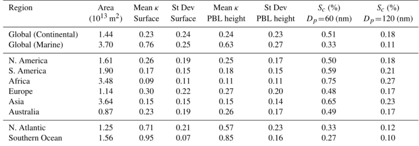
Table 5.Simulated global and regional annual meanκvalues (and standard deviation) at the surface and at the simulated PBL height under pre-industrial conditions. Standard deviation is calculated for the year from 5-hourly average data. Sc is the critical supersaturation (%),

calculated using the regional meanκat PBL height. Area column gives total land area for land sites, and marine area for marine sites.

Region Area Meanκ St Dev Meanκ St Dev Sc(%) Sc(%)

(1013m2) Surface Surface PBL height PBL height Dp=60 (nm) Dp=120 (nm)

Global (Continental) 1.44 0.23 0.24 0.24 0.23 0.51 0.18

Global (Marine) 3.70 0.76 0.25 0.63 0.27 0.33 0.11

N. America 1.61 0.26 0.19 0.25 0.17 0.50 0.18

S. America 1.90 0.17 0.15 0.18 0.15 0.59 0.21

Africa 3.48 0.09 0.11 0.11 0.11 0.75 0.27

Europe 1.14 0.30 0.22 0.27 0.20 0.48 0.17

Asia 3.64 0.15 0.15 0.15 0.14 0.65 0.23

Australia 0.87 0.23 0.19 0.26 0.17 0.49 0.17

N. Atlantic 1.25 0.71 0.21 0.57 0.23 0.33 0.12

Southern Ocean 1.56 0.95 0.07 0.85 0.16 0.27 0.10

The critical supersaturation (%) required to activate an aerosol of a particular size is also altered by present day emissions, for example the change inScrequired for a 60 nm

particle is (Sc Present−Sc Pre−industrial): +0.04 (N. Atlantic),

−0.04 (Europe),−0.14 (Africa),−0.11 (Asia). Overall Asia and Africa are the most sensitive regions a reduction inScof

≥17% due to present day emissions. Thus in polluted con-tinental regions, anthropogenic emissions not only increase the amount of aerosol present, but also increases the ease with which a particle of a particular size can activate.

The dominant effect of modern day emissions on CCN (and thus cloud droplet number) concentrations is the well documented increase in aerosol number and mass loading that has occurred since the industrial revolution. The change inκ, however, allows us to identify an additional, but more subtle effect. We find that the critical supersaturation re-quired to activate an aerosol of a particular size was system-atically different under pre-industrial conditions. However, the implications for this on CCN cannot be assessed without also considering the change in the aerosol number and size distribution that has occurred.

Thus, although particle size and number are the domi-nant factors in aerosol activation, we find that anthropogenic emissions have caused small but systematic differences in the water uptake ability of the aerosol, which may have implica-tions for the formation of clouds and precipitation. These changes are particularly important for mineral dust aerosols which are large enough to activate at low supersaturations, but are hydrophobic on emission and thus are sensitive to small changes inκ.

4 Conclusions

In this paper we show global fields of the κ hygroscopic-ity parameter developed by Petters and Kreidenweis (2007). Although κ has already been used in a range of field and modelling studies, to our knowledge this is the first time the global distribution ofκhas been presented. The global fields give us a number of insights into the water uptake ability of atmospheric aerosols. We find that:

– The simulated global meanκat the surface is 0.27±0.21 over land and 0.72±0.24 for marine regions, this agrees well with the estimates of Andreae and Rosenfeld (2008), although our study predicts a standard deviation of continentalκthat is double the previous estimate – The distribution ofκis found to be fairly uniform within

a region (as was suggested by field measurements), with regions of hundreds of kilometers showing little change inκ.

– There are, however, differencesbetweenregions which may be important. For example N. America and Eu-rope, which have a higher influence of sulfate and ni-trate aerosol have a meanκof 0.3 and 0.36 respectively, but African and S. American aerosol are less hygro-scopic (κ=0.15, 0.17). This implies that if an estimated value ofκ must be used, a continental-scaleκ is more appropriate than a global one.

(13)

– The variation ofκin the vertical can be important, par-ticularly in marine regions which consistently show a strong decrease in κ with altitude. In continental re-gions the vertical gradient is not so strong and varies between regions.

– The standard deviation of κ within a region mostly arises from variations in the horizontal distribution, and to a much lesser degree due to temporal variability. The exception to this is the N. Atlantic and N. America, which show larger temporal variability. This variabil-ity is well captured by monthly mean values, implying that the temporal variation arises from seasonal (and not shorter term) variations.

– The global distribution ofκ under pre-industrial con-ditions is different from present dayκ. Although this effect of the change in aerosol chemistry on CCN is small compared to the effect of the increase in aerosol loading with the anthropogenic emissions, it is interest-ing to note that under pre-industrial conditions the same aerosol number and size distribution would give a dif-ferent CCN loading. In summary, we find that under pre-industrial conditions, some marine regions (particu-larly the Gulf of Mexico) had higherκ values and thus were more able to activate at a particular supersatura-tion, while the converse is true for continental regions where anthropogenic pollution tends to increaseκ, and thus increase the ease with which a particle of a partic-ular size activates.

Acknowledgements. The authors would like to thank Hang Su at the MPI Chemistry for the useful discussion and collaboration. We also wish to thank colleagues at the MPI including Patrick J¨ockel, Benedikt Steil, Astrid Kerkweg and Andreas Baumg¨artner for help with the EMAC model. We acknowledge support by the European Research Council through the C8 project.

Further we thank Julian Wilson and Elisabetta Vignatti (JRC, Ispra) for the M7 model, Philip Stier for its implementation in ECHAM5, Frank Dentener (JRC) and the former partners of the EU-project PHOENICS (http://phoenics.chemistry.uoc.gr/) for many fruitful discussions, and Swen Metzger for the initial development of GMXe.

The service charges for this open access publication have been covered by the Max Planck Society.

Edited by: J. Quaas

References

Allan, J. D., Baumgardner, D., Raga, G. B., Mayol-Bracero, O. L., Morales-Garca, F., Garca-Garca, F., Montero-Martnez, G., Bor-rmann, S., Schneider, J., Mertes, S., Walter, S., Gysel, M., Dusek, U., Frank, G. P., and Krmer, M.: Clouds and aerosols in Puerto Rico−a new evaluation, Atmos. Chem. Phys., 8, 1293–1309, 2008, http://www.atmos-chem-phys.net/8/1293/2008/.

Andreae, M. O. and Rosenfeld, D.: Aerosol-cloud-precipitation interactions. Part 1. The naturea and sources of cloud-active aerosols, Earth. Sci. Rev.,89, doi:10.1016/j.earscirev.2008.03.001, 2008.

Bauer, S. E., Mishchenko, M. I., Lacis, A. A., Zhang, S., Perlwitz, J., and Metzger, S. M.: Do sulfate and nitrate coatings on mineral dust have important effects on radiative properties and climate modeling?, J. Geophys. Res.-Atmos., 112, D06307, doi:10.1029/ 2005JD006977, 2007.

Bougiatioti, A., Fountoukis, C., Kalivitis, N., Pandis, S. N., Nenes, A., and Mihalopoulos, N.: Cloud condensation nuclei measure-ments in the marine boundary layer of the Eastern Mediter-ranean: CCN closure and droplet growth kinetics, Atmos. Chem. Phys., 9, 7053–7066, 2009,

http://www.atmos-chem-phys.net/9/7053/2009/.

Broekhuizen, K., Chang, R.-W., Leaitch, W. R., Li, S.-M., and Ab-batt, J. P. D.: Closure between measured and modeled cloud condensation nuclei (CCN) using size-resolved aerosol composi-tions in downtown Toronto, Atmos. Chem. Phys., 6, 2513–2524, 2006, http://www.atmos-chem-phys.net/6/2513/2006/.

Chang, R. Y.-W., Slowik, J. G., Shantz, N. C., Vlasenko, A., Liggio, J., Sjostedt, S. J., Leaitch, W. R., and Abbatt, J. P. D.: The hygro-scopicity parameter (κ) of ambient organic aerosol at a field site subject to biogenic and anthropogenic influences: relationship to degree of aerosol oxidation, Atmos. Chem. Phys., 10, 5047– 5064, doi:10.5194/acp-10-5047-2010, 2010.

Cubison, M. J., Ervens, B., Feingold, G., Docherty, K. S., Ulbrich, I. M., Shields, L., Prather, K., Hering, S., and Jimenez, J. L.: The influence of chemical composition and mixing state of Los Angeles urban aerosol on CCN number and cloud properties, At-mos. Chem. Phys., 8, 5649–5667, 2008,

Dentener, F., Kinne, S., Bond, T., Boucher, O., Cofala, J., Generoso, S., Ginoux, P., Gong, S., Hoelzemann, J. J., Ito, A., Marelli, L., Penner, J. E., Putaud, J.-P., Textor, C., Schulz, M., van der Werf, G. R., and Wilson, J.: Emissions of primary aerosol and precur-sor gases in the years 2000 and 1750, prescribed data-sets for AeroCom , Atmos. Chem. Phys., 6, 4321–4344, 2006,

Dusek, U., Frank, G. P., Hildebrandt, L., Curtius, J., Schneider, J., Walter, S., Chand, D., Drewnick, F., Hings, S., Jung, D., Bor-rmann, S., and Andreae, M. O.: Size Matters More Than Chem-istry for Cloud-Nucleating Ability of Aerosol Particles, Science, 312, 1375–1378, doi:10.1126/science.1125261, 2006.

Dusek, U., Frank, G. P., Curtius, J., Drewnick, F., Schneider, J., K¨uurten, A., Rose, D., Andreae, M. O., Borrmann, S., , and P¨oschl, U.: Enhanced organic mass fraction and decreased hy-groscopicity of cloud condensation nuclei (CCN) during new particle formation events, Geophys. Res. Lett., 37, L03804, doi:10.1029/2009GL040 930, 2010.

(14)

dis-tribution of reactive trace gases, J. Geophys. Res.-Atmos., 100, 20999–21012, doi:http://dx.doi.org/10.1029/95JD02266, 1995. Guibert, S., Snider, J. R., and Brenguier, J.-L.: Aerosol

activa-tion in marine stratocumulus clouds: 1. Measurement valida-tion for a closure study, J. Geophys. Res. - Atmos., 108, 8628, doi:10.1029/2002JD002678, 2003.

Gunthe, S. S., King, S. M., Rose, D., Chen, Q., Roldin, P., Farmer, D. K., Jimenez, J. L., Artaxo, P., Andreae, M. O., Martin, S. T., and P¨oschl, U.: Cloud condensation nuclei in pristine tropi-cal rainforest air of Amazonia: size-resolved measurements and modeling of atmospheric aerosol composition and CCN activity, Atmos. Chem. Phys., 9, 7551–7575, 2009,

Holtslag, A. A. M. and Boville, B. A.: Local Versus Nonlocal Boundary-Layer Diffusion in a Global Climate Model., J. Clim., 6, 1825–1842, 1993.

Holtslag, A. A. M., de Bruijn, E. I. F., and Pan, H.-L.: A high res-olution air mass transformation model for short-range weather forecasting, Mon. Weather Rev., 118, 1561–1575, 1990. Hudson, J. G.: Variability of the relationship between particle size

and cloud-nucleating ability, Geophys. Res. Lett., 34, L08801, doi:10.1029/2006GL028850, 2007.

J¨ockel, P., Sander, R., Kerkweg, A., Tost, H., J., and Lelieveld, J.: Technical Note: The Modular Earth Submodel System (MESSy) – a new approach towards Earth System Modeling, Atmos. Chem. Phys., 5, 433–444, 2005,

Jöckel, P., Tost, H., Pozzer, A., Brühl, C., Buchholz, J., Ganzeveld, L., Hoor, P., Kerkweg, A., Lawrence, M., Sander, R., Steil, B., Stiller, G., Tanarhte, M., Taraborrelli, D., van Aardenne, J., and Lelieveld, J.: The atmospheric chemistry general circulation model ECHAM5/MESSy1: consistent simulation of ozone from the surface to the mesosphere, Atmos. Chem. Phys., 6, 5067– 5104, 2006, http://www.atmos-chem-phys.net/6/5067/2006/. Kandler, K. and Shütz: Climatology of the Average Water-soluble

Volume Fraction of Atmospheric Aerosol, Atmos. Res, 07, 77– 92, 2007.

Kerkweg, A., Buchholz, J., Ganzeveld, L., Pozzer, A., Tost, H., and J¨ockel, P.: Technical Note: An implementation of the dry removal processes DRY DEPosition and SEDImentation in the Modular Earth Submodel System (MESSy), Atmos. Chem. Phys., 6, 4617–4632, 2006a.

Kerkweg, A., Sander, R., Tost, H., and J¨ockel, P.: Technical note: Implementation of prescribed (OFFLEM), calculated (ON-LEM), and pseudo-emissions (TNUDGE) of chemical species in the Modular Earth Submodel System (MESSy), Atmos. Chem. Phys., 6, 3603–3609, 2006b.

Kerkweg, A., J¨ockel, P., Tost, H., Sander, R., Schulz, M., Stier, P., Vignati, E., Wilson, J., and Lelieveld, J.: Consistent simula-tion of bromine chemistry from the marine boundary layer to the stratosphere. Part 1: Model description, sea salt aerosols and pH, Atmos. Chem. Phys., 8, 5899–5917, 2008,

Kim, D., Wang, C., Ekman, A. M. L., Barth, M. C., and J., R. P.: Distribution and direct radiative forcing of carbonaceous and sulfate aerosols in an interactive size-resolving aerosolclimate model, J. Geophys. Res.-Atmos., 113, doi:10.1029/2007JD009756, 2008.

King, S. M., Rosenoern, T., Shilling, J. E., Chen, Q., Wang, Z.,

Biskos, G., McKinney, K. A., P¨oschl, U., and Martin, S. T.: Cloud droplet activation of mixed organic-sulfate particles pro-duced by the photooxidation of isoprene, Atmos. Chem. Phys., 10, 3953–3964, 2010,

Mikhailov, E., Vlasenko, S., Martin, S. T. Koop, T., and P¨oschl, U.: Amorphous and crystalline aerosol particles interacting with wa-ter vapor: conceptual framework and experimental evidence for restructuring, phase transitions and kinetic limitations, Atmos. Chem. Phys., 9, 9491–9522, 2009,

Morgan, W. T., Allan, J. D., Bower, K. N., Capes, G., Crosier, J., Williams, P. I., and Coe, H.: Vertical distribution of sub-micron aerosol chemical composition from North-Western Europe and the North-East Atlantic, Atmos. Chem. Phys., 5389–5401, 2009. Niedermeier, D., Wex, H., Voigtl¨ander, J., Stratmann, F., Br¨uggemann, E., Kiselev, A., Henk, H., and Heintzenberg, J.: LACIS-measurements and parameterization of sea-salt particle hygroscopic growth and activation, Atmos. Chem. Phys., 8, 579– 590, 2008, http://www.atmos-chem-phys.net/8/579/2008/. Petters, M. D. and Kreidenweis, S. M.: A single parameter

repre-sentation of hygroscopic growth and cloud condensation nucleus activity, Atmos. Chem. Phys., 7, 1961–1971, 2007,

P¨oschl, U., Rose, D., and Andreae, M. O.: Climatologies of Cloudrelated Aerosols - Part 2: Particle Hygroscopicity and Cloud Condensation Nuclei Activity, in: Clouds in the Perturbed Climate System, edited by: Heintzenberg, J. and Charlson, R. J., MIT Press, Cambridge, ISBN 978-0-262-012874, 58–72, 2009. Pringle, K. J., Tost, H., Metzger, S., Steil, B., Giannadaki, D.,

Nenes, A., Fountoukis, C., Stier, P., Vignati, E., and Lelieveld, J.: Description and evaluation of GMXe: a new aerosol sub-model for global simulations (v1), Geosci. Model Dev. Discuss., 3, 569–626, doi:10.5194/gmdd-3-569-2010, 2010.

Reutter, P., Su, H., Trentmann, J., Simmel, M., Rose, D., Gunthe, S. S., Wernli, H., Andreae, M. O., and P¨oschl, U.: Aerosol-and updraft-limited regimes of cloud droplet formation: influ-ence of particle number, size and hygroscopicity on the activa-tion of cloud condensaactiva-tion nuclei (CCN), Atmos. Chem. Phys., 9, 7067–7080, 2009,

Roeckner, E., Brokopf, R., Esch, M., Giorgetta, M., Hagemann, S., Kornblueh, L., Manzini, E., Schlese, U., and Schulzweida, U.: Sensitivity of simulated climate to horizontal and vertical resolution in the ECHAM5 atmosphere model, J. Climate, 19, 3371–3791, doi:10.1175/JCLI3824.1, 2006.

Rose, D., Gunthe, S. S., Mikhailov, E., Frank, G. P., Dusek, U., Andreae, M. O., and U, P.: Calibration and measurement uncertainties of a continuous-flow cloud condensation nuclei counter (DMT-CCNC): CCN activation of ammonium sulfate and sodium chloride aerosol particles in theory and experiment, Atmos. Chem. Phys., 8, 1153–1179, 2008,

(15)

Ruehl, C. R., Chuang, P. Y., and Nenes, A.: Distinct CCN activation kinetics above the marine boundary layer along the California coast, Geophys. Res. Lett., 36, L15814, doi:10.1029/2009GL038 839, 2009.

Sander, R., Kerkweg, A., J¨ockel, P., and Lelieveld, J.: Technical note: The new comprehensive atmospheric chemistry module MECCA, Atmos. Chem. Phys., 5, 445–450, 2005,

Shinozuka, Y., Clarke, A. D., DeCarlo, P. F., Jimenez, J. L., Dunlea, E. J., Roberts, G. C., Tomlinson, J. M., Collins, D. R., How-ell, S. G., Kapustin, V. N., McNaughton, C. S., and Zhou, J.: Aerosol optical properties relevant to regional remote sensing of CCN activity and links to their organic mass fraction: airborne observations over Central Mexico and the US West Coast dur-ing MILAGRO/INTEX-B, Atmos. Chem. Phys., 9, 6727–6742, 2010, http://www.atmos-chem-phys.net/9/6727/2010/.

Snider, J. R. and Petters, M. D.: Optical particle counter mea-surement of marine aerosol hygroscopic growth, Atmos. Chem. Phys., 8, 1949–1962, 2008,

Spracklen, D. V., Carslaw, K. S., Kulmala, M., Kerminen, V. M., Sihto, S. L., Riipinen, I., Merikanto, J., Mann, G. W., Chip-perfield, M. P., Wiedensohler, A., Birmili, W., and Lihavainen, H.: Contribution of particle formation to global cloud conden-sation nuclei concentrations, Geophys. Res. Lett., 35, L06808, doi:10.1029/2007GL033038, 2008.

Stier, P., Feichter, J., Kinne, S., Kloster, S., Vignati, E., Wilson, J., Ganzeveld, L., Tegen, I., Werner, M., Balkanski, Y., Schulz, M., Boucher, O., Minikin, A., and Petzold, A.: The aerosol-climate model ECHAM5-HAM, Atmos. Chem. Phys., 5, 1125– 1156, doi:10.5194/acp-5-1125-2005, 2005.

Tost, H., J¨ockel, P., and Lelieveld, J.: Influence of different convec-tion parameterisaconvec-tions in a GCM, Atmos. Chem. Phys., 6, 5475– 5493, 2006, http://www.atmos-chem-phys.net/6/5475/2006/. Tost, H., J¨ockel, P., Kerkweg, A., Pozzer, A., Sander, R.,

and Lelieveld, J.: Global cloud and precipitation chemistry and wet deposition: tropospheric model simulations with ECHAM5/MESSy1, Atmos. Chem. Phys., 7, 2733–2757, 2007a. Tost, H., J¨ockel, P., and Lelieveld, J.: Lightning and convection parameterisations – uncertainties in global modelling, Atmos. Chem. Phys., 7, 4553–4568, 2007b.

Tsigaridis, K., Krol, M., Dentener, F. J., Balkanski, Y., Lathi`ere, J., Metzger, S., Hauglustaine, D. A., and Kanakidou, M.: Change in global aerosol composition since preindustrial times, Atmos. Chem. Phys., 6, 5143–5162, 2006,

Van Aardenne, J., Dentener, F., Olivier, J., Klein Goldewijk, C., and Lelieveld, J.: A High Resolution Dataset of Historical Anthro-pogenic Trace Gas Emissions for the Period 1890-1990, Global Biogeochem. Cy., 15, 909–928, 2001.

Vestin, A., Rissler, J., Swietlicki, E., Frank, G. P., and An-dreae, M. O.: Cloud-nucleating properties of the Amazonian biomass burning aerosol: Cloud condensation nuclei measure-ments and modeling, J. Geophys. Res.-Atmos., 112, D14201, doi:10.1029/2006JD008104, 2007.

Vignati, E., Wilson, J., and Stier, P.: M7: An efficient size-resolved aerosol microphysics module for large-scale aerosol transport models, Journal of Geophysical Research, 109, D22202, doi: http://dx.doi.org/10.1029/2003JD004485, 2004.

Wang, J., Lee, Y.-N., Daum, P. H., Jayne, J., and Alexander, M. L.: Effects of aerosol organics on cloud condensation nucleus (CCN) concentration and first indirect aerosol effect, Atmos. Chem. Phys., 8, 6325–6339, 2008,

Wex, H., Petters, M. D., Carrico, C. M., Hallbauer, E., Massling, A., McMeeking, G. R., Poulain, L., Wu, Z., Kreidenweis, S. M., and Stratmann, F.: Towards closing the gap between hygroscopic growth and activation for secondary organic aerosol: Part 1 – Evidence from measurements, Atmos. Chem. Phys., 9, 3987– 3997, 2009, http://www.atmos-chem-phys.net/9/3987/2009/. Wex, H., McFiggans, G., Henning, S., and Stratmann, F.: Influence

of the external mixing state of atmospheric aerosol on derived CCN number concentrations, Geophys. Res. Lett., 37, L10805, doi:10.1029/2010GL043 337, 2010.