TOPOGRAPHIC ASPECTS IN THE SPATIAL AND TEMPORAL DYNAMIC OF NET RADIATION
Doi:http://dx.doi.org/10.1590/1809-4430-Eng.Agric.v37n5p1028-1040/2017
ROBERTO FILGUEIRAS1*, DONIZETI A. P. NICOLETE2, TÂNIA M. DE CARVALHO3,
ANTONIO R. DA CUNHA2, CÉLIA R. L. ZIMBACK2
1*Corresponding author. Universidade Federal de Viçosa, Departamento de Engenharia Agrícola/ Viçosa - MG, Brasil.
E-mail: [email protected]
ABSTRACT: The measurements obtained by remote sensing are influenced by issues related to relief. Based on that, this paper aims to analyze the spatial and temporal dynamics of the net radiation (Rn), considering the influence of topographic parameters on it, in Edgárdia Experimental Farm (FEE). It was used the methodology based on the SEBAL algorithm (Surface Energy Balance Algorithm for Land) to estimate the net radiation by orbital images. In order to assess the topographic influence on the computing of net radiation, three methodologies were applied: without topographic correction (RnSem), cosine correction (RnCos) and C correction (RnC). These methodologies were applied on 21 images of the orbital platform Landsat-5/TM, from 1985 up to 2010. Due to the complex relief of the FEE, the cosine correction did not show effectiveness on the attenuation of topographic influence. For the values of RnC, we noticed an average reduction of 5.97% for the standard deviation, relative to the images without correction. These results show the importance of considering the relief, to achieve higher accuracies on the estimation of biophysical parameters with orbital images.
KEYWORDS: topographic correction, SEBAL, biophysical parameters.
INTRODUCTION
Biophysical parameters obtaining through remote sensing has been of great value for the decision making of public agencies and rural companies. A large number of researchers in the area of Agrarian Science have used geotechnologies in recent years to better understand the spatial dynamics of their studies (Andrade et al., 2014; Di Pace et al., 2008; Li et al., 2013; Lima et al., 2012; Menezes et al., 2009; Oliveira et al., 2014; Santos et al., 2014; Silva et al., 2005 and Sousa, 2014).
However, when using orbital images in order to acquire information about vegetation parameters, it must take into account the possible interferences that may be present in the images and result in inaccurate estimates of the parameters. Thus, obtaining consistent values with orbital images depends on the radiometric quality of the data which is directly related to the atmospheric interferences and to the surface illumination conditions (slope areas) at the moment of the satellite passage (Lima & Ribeiro, 2014; Richter, 1998). Thus, it is necessary to attenuate these interferences, mainly in multitemporal studies that are related to the classification of the soil cover and biophysical parameters obtaining from the environment. Therefore, when the objective is to evaluate the dynamics of a given phenomenon over time, there is a need to homogenize the external conditions to the analysis (Chavez Jr., 1988; Hantson & Chuvieco, 2011; Ponzoni et al., 2012).
The radiometric interferences on the images in areas of heterogeneous relief make a homogeneous culture respond in different ways in the field depending on the position that it is on the surface. The reading of the orbital sensor for shaded areas, underestimates the spectral response of an object, whereas the exposed area to the Sun tend to have an inverse response (Riaño et al., 2003). According to Schulmann et al. (2015), the same soil use undergoes variability due to the aspect (inclined surface azimuth) and slope, being an obstacle in obtaining the reflectances of these surfaces.
Several methods have been proposed to mitigate the soil topography effects have on the accuracy of the digital processes, with the use of satellite images (Balthazar et al., 2012; Kara et al., 2014; Meyer et al., 1993; Szantoi & Simonetti, 2013; Teillet et al., 1982). Among them are the Lambertian methods which consider the surface to be isotropic, and the non-Lambertian methods whose surfaces are analyzed as anisotropic.
In order to estimate the radiation balance with greater accuracy due to its importance in the energy balance equation and, consequently, in the estimation of crop evapotranspiration, this study had as objective to analyze the spatial dynamics along a temporal series of radiation balance in the Edgárdia Experimental Farm, taking into account the topographical aspects of it, which has an uneven soil, using in this analysis two methods of topographical correction: a Lambertian and a non-Lambertian method.
MATERIAL AND METHODS Study area
The study was carried out at the Edgárdia Experimental Farm (FEE), located in the city of
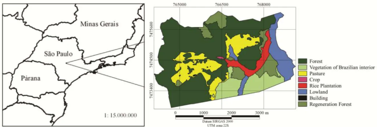
Botucatu, State of São Paulo (Figure 1), which belongs to the Agronomic SciencesCollege (FCA)
of the Universidade Estadual Paulista Júlio de Mesquita Filho (UNESP). It has an area of about 1,200 ha, with an altitude varying between 475 and 725 meters, which is delimited by the geographical coordinates: 48°25'36.25"W and 22°48'2.80"S; 22°49'52.36"S and 48°22'37.46"W, datum WGS-84.
According to Cunha & Martins (2009) the climate of the region is Cfa (temperate hot mesothermal) humid with an average annual temperature of 20.3°C and an average annual rainfall of 1,428 mm. The average temperature of the coldest month (July) is 17.1° C and the hottest month (February) is 23.1 ° C. The months with extreme rainfall are January (more rainy) and August (drier).
FIGURE 1. Location and land use in the Edgárdia Experimental Farm.
Data processing
All data processing as well as the elaboration of the research database was carried out using as support tools the geographic information systems: SPRING 5.1.8 - Geographic Information
Processing System (Camara et al., 1996); GRASS GIS 7.0 – Geographic Resources Analysis
Support System (GRASS Development Team, 2015) and QGIS 2.8 (QGIS Development Team,
2015).
In order to perform the research, 21 images (Table 1) of the LANDSAT-5 satellite, TM sensor (Thematic Mapper) were used in clear sky days, corresponding to orbit / point 220/076, according
to the global notation acquisition system WRS-2 (Worldwide Reference System) data from Landsat
program. The images were acquired in the USGS (United States Geological Survey) database,
which were orthorectified at the Standart Terrain correction Level 1T or Level 1G processing level
(USGS, 2014).
TABLE 1. Characteristics of the used images in the study.
Date Day of the year Cloud Cover Azimuth angle Solar elevation angle Time of passage
09/11/1985 254 1% 57.58 44.38 09:39:52
09/14/1986 257 0% 60.37 43.50 09:31:06
09/27/1988 271 0% 63.49 49.53 09:41:11
09/12/1991 255 0% 59.01 43.42 09:34:23
09/30/1992 274 13% 66.61 48.55 09:32:18
09/20/1994 263 0% 63.44 44.45 09:26:57
09/12/1997 255 4% 57.30 45.29 09:42:52
09/29/1997 271 4% 63.32 50.24 09:43:19
08/01/1999 213 24% 45.01 34.82 09:48:14
09/02/1999 245 0% 52.89 42.97 09:47:41
08/19/2000 232 15% 49.21 39.21 09:48:14
08/06/2001 218 1% 45.58 36.38 09:50:51
08/12/2003 224 7% 47.51 37.10 09:47:26
08/14/2004 227 0% 46.79 38.82 09:53:31
08/17/2005 229 0% 46.33 40.37 09:58:34
08/04/2006 216 29% 42.20 37.98 10:03:49
08/23/2007 235 2% 46.31 42.86 10:03:49
09/08/2007 251 0% 50.80 47.80 10:03:41
08/25/2008 238 0% 48.88 42.35 09:56:11
09/10/2008 253 1% 53.73 47.22 09:55:44
The estimate of the spatial-temporal series of the radiation balance was processed in three stages: one without the topographic characteristics of the soil (without the products derived from the digital elevation model), and two with the use of them. In this way, two topographic correction methods developed by Teillet et al. (1982) were applied to the images: the cosine and the C correction method.
Before the topographic correction, the images were submitted to the radiometric calibration and to the atmospheric correction with the conversion of the digital numbers of images to physical correspondents, in this case, surface reflectance (Ponzoni et al., 2012).
Topographic corrections were applied to the surface reflectance data of all bands, except for band 6, relative to the thermal wavelength of the 21 time series images.
Firstly, to perform the topographic correction process in the images it was necessary to calculate the angle of solar incidence which is relative to the normal of each pixel on the surface. For this it was necessary to construct a digital elevation model, elaborated from the IGC
planialtimetricchart, in scale of 1: 10,000 and vertical equidistance between curves of level of 5m.
For the elaboration of the model it was necessary to vectorize the curve level of the study area, so that then it was used the TIN (Triangular Irregular Network) interpolation method, with spatial
resolution compatible to TM sensor images. After obtaining the MDE were calculated the slope angle and the azimuth angle of the inclined surface, both calculated according to the methodology
by Horn (1981). The angle of solar incidence for each pixel was computed according to [eq. (1)]
(Colby, 1991; Moreira & Valeriano, 2014).
(1)
where,
θs represents the solar Zenith angle at the time the satellite passes;
ηi the angle of surface inclination;
ϕa the azimuthal solar angle, and
ϕo the orientation angle of the inclined surface.
The azimuthal and zenithal angles were obtained in the metadata files of the images, considering a single pair of angles for each image, since they vary little in a scene of the TM sensor of the Landsat-5 satellite (Hantson & Chuvieco, 2011).
The Cosine correction was a methodology proposed by Teillet et al. (1982), and since then, has been used for the topographical correction of satellite images. The corrected images obtaining by this method was performed according to [eq. (2)].
(2) where,
ρh is defined as the reflectance on a horizontal surface after the removal of the topographic effects;
ρT the surface reflectance with the interference of the soil before the topographic correction
process;
θz the solar Zenith angle at the time the satellite passes, and
γi is the angle of solar incidence for each point on the Earth's surface.
(3) where,
factor C is a constant (calculated with Equation 4) derived from the correlation between Cosγi
and each of the spectral bands of the used images in the study, and it is necessary to stratify by date of the images the surfaces with spectral similarity.
(4)
Being:
m the angular coefficient of the generated equation from the correlation between the two factors, and
b the intercept on the y-axis of this correlation (Equation 5).
(5) where,
ρT is the dependent variable, and
cosγi is the independent variable.
In order to stratify the surfaces with the highest spectral similarity at each date, necessary for correction C, images of the NDVI vegetation index were used for the 21 dates, where a bound of 0.4 was established as the change of absence for vegetation presence in a pixel; methodology used in the studies of Hantson & Chuvieco (2011) and Lima & Ribeiro (2014).
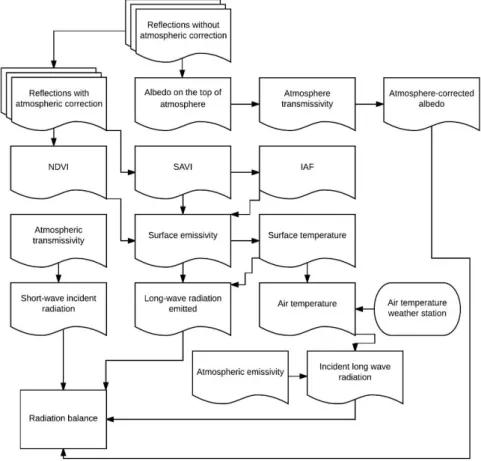
After the different techniques for the approaches proposed in this study, the radiation balance
(Equation 6) was obtained for the different methodologies, using the SEBAL algorithm - Surface
Energy Balance Algorithm for Land (Figure 2) (Allen et al., 2002).
(6)
where,
Rs ↓ is the short-wave radiation incident on the surface;
α the corrected pixel albedo;
RL ↓ is the long-wave radiation emitted by the atmosphere;
RL the long-wave radiation emitted by the pixel (surface) and
FIGURE 2. Flowchart of the SEBAL methodology to obtain the radiation balance at the Edgárdia Experimental Farm, in the city of Botucatu-SP.
RESULTS AND DISCUSSION
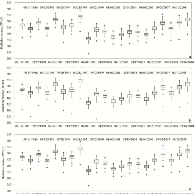
FIGURE 3. Boxplot of RnSem (a), RnCos (b) and RnC (c) for FEE, over the studied series time.
It was verified, by means of Figure 3b, that the cosine correction drastically modified the values of radiation balance in the FEE for some pixels in addition to observing that on the dates 08/01/1999 and 08/06/2001, saturated pixel or with unrealistic values of RnCos were found. In this method of correction, Teillet et al. (1982) considered that the terrestrial targets were isotropic reflectors, that is, they reflected in a homogeneous way in all directions, a characteristic that, in most cases, is not found in nature. According to the same authors, the cosine correction would have greater applicability in soil that have slopes lower than 25 ° and lighting angles smaller than 45 °. The FEE soil, based on the digital elevation model, shows slope values above 25 °. When analyzing
the images of lighting angles ( for the workdates it was verified that in all images were
observed superior to 45 °.
The pixels that presented saturation (unreal values of RnCos) had values of illumination
angles ( in relation to the normal surface, higher than 69.62 °, reaching angles of up to 76.11 °,
angle close to or greater than 90 °, i.e. low cos . These authors found overcorrections for the cosine methodology in areas with low cosine of the lighting angle, which was also verified by FEE.
Hatson & Chuvieco (2011) evaluated different methods of topographic correction in Landsat / ETM+ images. When reporting on the cosine correction theses researchers stated that this correction is not able to correct scenes in poor lighting conditions, situation found for some regions of the FEE.
Therefore, problems were detected when performing the topographic correction of the cosine type for the FEE, which may be related to the complexity of its soil. According to Meyer et al. (1993), the cosine correction is often used for relatively flat soil with no complexities, in order to equalize the differences related to lighting due to the different positions that the sun assumes in multitemporal studies. According to the same authors, the cosine correction for poorly illuminated areas presents greater disproportions in the attenuation of images parameters.
According to Teillet et al. (1982) and Meyer et al. (1993), correction C is a modification of the cosine correction with the addition of a factor C, which aims to model the diffuse radiation reaching the surface. It was not observed for the RnC discrepancies in the Rn values, which can be verified in Figure 3. For this correction, the values of radiation balance presented amplitude of
241.10 W m-² (08/01/1999) to 591.94 W m-² (09/29/1997). The average values of RnC in the FEE
for the analyzed dates presented amplitude of 361.77 W m-² (08/01/1999) to 536.39 W m-²
(09/28/1997).
Wu et al. (2008), using four topographic correction methodologies found that the cosine correction greatly modified the spatial dispersion of the spectral radiance values, while the C correction did not present significant changes in the histogram of the values. These results are in agreement with those found in the present study, that is, abrupt changes in the histogram of RnCos values when compared with RnSem and small difference in amplitude and RnC histogram values when compared with the histogram of RnSem. However to determine whether these corrections were efficient or not, it is necessary to analyze more statistical parameters.
Since this interference of the topography does not occur in an egalitarian way in the scene, the tendency is that, after attenuation, the variability of the data becomes smaller (Hatson & Chuvieco, 2011). The standard deviation analysis of the images that went through correction, it can be seen that the values of RnCos did not present, at any studied date, the standard deviation inferior to the data of RnSem, proving that for FEE, the cosine correction was not effective.
When analyzing the standard deviation data for the C correction (RnC) it was observed that in 90% of the dates this method reduced the variability of the data (Figure 3c). The images corrected by the C method that did not present standard deviations lower than the images without correction, were those on 09/27/1998 and 09/16/2010. Even so, it can be considered that the C correction was effective in attenuating the topography effects for FEE, because, on most dates, there was reduction of the standard deviation and, consequently, reduction of the randomness caused by the soil. The mean reduction of the standard deviation of the uncorrected images for the corrected images by the C correction was 5.97%. Lima et al. (2012), testing different topographic correction methods in Landsat-5 / TM images, observed that there was also a reduction on the standard deviation of the corrected reflectance images for the uncorrected ones. The average reduction, found by these authors was 10.4%, which attributed this reduction as an indication of the normalization on the corrected reflectances. It is worth noting that the average reduction of the standard deviation found in the present study was for the values of radiation balance and not for the reflectances, as in the study by Lima & Ribeiro (2014).
method of C correction was superior to the cosine correction. Both conclusions of these authors are in agreement with the one found in the present study.
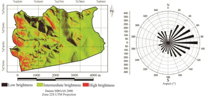
In order to discuss and illustrate the interference that the soil exerts on the radiation balance maps it was performed a shading of the FEE soil (Figure 4), on 09/11/1985, at the time of the satellite passage (09h39min). By that date, the Sun had an azimuth of 57.58° and a solar elevation angle of 44.37 °. In Figure3 is presented the polar histogram of the azimuth on the inclined surface of the pixels present in FEE.
FIGURE 4. Shaded soil at Edgárdia Experimental Farm on 09/11/1985 and polar histogram of the azimuth angle on the inclined surface.
The information in Figure 4 is intended to complement the analyzes of the influence of the topography on the images of the radiation balances, since this allows to identify the more and less illuminated areas at the moment of the passage of the satellite to the FEE region. The portions in Figure 4 which are in the reddish coloration were receiving direct radiation from the Sun and were therefore well illuminated, unlike the dark colored portions.
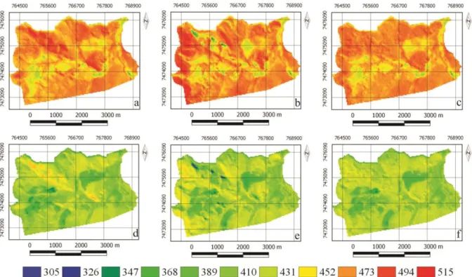
FIGURE 5. Images of the radiation balance (W / m²), without topographic correction (a and d), with cosine correction (b and e) and C correction (c and f) referring to 09/11/1985 and 08/17/2005.
Note the influence that the topography exerts on the values of radiation balance, since in observing Figure 5 (a and d), considering the images of Rn that were not corrected topographically, it was found regional tendency of high values on Rn at the time of the satellite passage. This portion extends from the northwest to the southeast of these maps, the same region that in Figure 4 is shaded or with low light. This is a region that is predominantly oriented towards azimuthal angles between 135 ° and 225 ° (mostly), that is, predominantly perpendicular to the sun's rays, occurring also in this region the presence of angles between 225 ° to 315 °, opposite to the solar rays. In this way, it can be seen that the shading occurred in this region, masked the reflective characteristics of the use soil present on this surface. Balthazar et al. (2012) found similar behavior in the Himalayan mountains in western Bhutan, where steep valleys are oriented perpendicular to the Sun's direction of illumination. These authors found that for these sites the images had a dark appearance, proving the effect of the topography on this region.
According to Jorge & Sartori (2002) who carried out a land use mapping for FEE, the region with surface shading is composed of a semideciduous seasonal forest. This shading made this surface no longer exhibit a spectral behavior typical of vegetation, to assume a more absorptive behavior of solar radiation. Thus, whether more radiation is absorbed in counterpart to the reflected one, a higher radiation balance is expected in this place, and therefore, these shaded regions presented with higher radiation balances than the others for the FEE. The Rn values on this map surface are higher than in other portions of the FEE that have the same land use. Riaño et al. (2003) reported that the effects of topography induce variations in the reflectance of the same land use, causing the same vegetation to have, in shaded areas, less reflective behavior than in illuminated areas, which is in agreement with the observed for FEE.
is noticed that the radiation balance maps for FEE no longer show the trend related to surface shading. Visually, the trend that occurred in the northwest-southeast portion was eliminated from the FEE. This result was found for the remaining years.
In general it was verified that the faces facing East and West were the ones that presented the highest relative errors when compared with RnSem and RnC, and the surfaces facing East were those that directly received solar energy, and those facing West were opposite to the direction of the sun's rays.
CONCLUSIONS
According to the processing performed for FEE, in order to analyze the influence degree of the topography in these parameters we concluded that:
The cosine correction was not able to effectively correct areas with low luminosity, where
was found pixels with significant overcorrections of the values for this methodology.
Correction C was adequate according to qualitative and quantitative parameters, being able
to correct the effects of the topography on the values of radiation balance in the FEE;
After the data analysis, the soil interference must be taken into account in the processing of
orbital images, being fundamental to achieve greater accuracy in the estimation of products derived from remote sensing.
REFERENCES
Allen RG, Tasumi M, Trezza R, Waters R, Bastiaassen W (2002) Surface Energy Balance
Algorithm for Land (SEBAL) - Advanced training and User’s Manual. Kimberly, Idaho
Implementation. 98p.
Andrade RG, Sediyama G, Soares PV, Gleriani JM, Menezes SJMC (2014) Estimativa da produtividade da cana-de-açúcar utilizando o Sebal e imagens Landsat. Revista Brasileira de
Meteorologia 29(3):433-442.
Balthazar V, Vanacker V, Lambin EF (2012) Evaluation and parameterization of ATCOR3
topographic correction method for forest cover mapping in mountain areas. International Journal of
Applied Earth Observation and Geoinformation 18:436-450.
Camara G, Souza RCM, Freitas UM, Garrido J, Mitsuo Junior F (1996) Spring: integrating remote
sensing and GIS by object oriented data modelling. Computers & Graphics 20(3):395-403.
Carvalho WA, Panoso LA, Moraes MH (1991) Levantamento semidetalhado dos solos da Fazenda
Experimental Edgardia – Município de Botucatu. Botucatu, Faculdade de Ciências Agronômicas,
Universidade Estadual Paulista. 467p.
Chavez Jr PS (1988) An improved dark-object subtraction technique for atmospheric scattering
correction of multispectral data. Remote Sensing of Environment 24(3):459-479.
Colby JD (1991) Topographic normalization in rugged terrain. Phtogrammetric Engineering &
Remote Sensing 57(5):531-537.
Cunha AR, Martins D (2009) Classificação climática para os municípios de Botucatu e São Manuel, SP. Irriga 14(1):1-11.
Di Pace FT, Silva BB, Silva VPR, Silva STA (2008) Mapeamento do saldo de radiação com imagens Landsat 5 e modelo de elevação digital. Revista Brasileira de Engenharia Agrícola e
Ambiental 12(4):385-392.
GRASS Development Team (2015) Geographic Resources Analysis Support System (GRASS) Software, Version 7.0. Open Source Geospatial Foundation. Available: http://grass.osgeo.org. Hantson S, Chuvieco E (2011) Evaluation of different topographic correction methods for Landsat
imagery. International Journal of Applied Earth Observation and Geoinformation 13(5):691-700.
Horn BKP (1981) Hill shading and the reflectance map. Proceedings of the IEEE 69(1):14-47.
Li Z et al. (2013) Retrieval of the surface evapotranspiration patterns in the alpine grassland –
wetland ecosystem applying SEBAL model in the source region of the Yellow River, China.
Ecological Modelling 270:64-75.
Lima RNdeS, Ribeiro CBdeM (2014) Comparação de métodos de correção topográfica em imagens
Landsat sob diferentes condições de iluminação. Revista Brasileira de Cartografia 66(5):1097-1116.
Lima EDP, Sediyama GC, Silva BBD, Gleriani JM, Soares VP (2012) Seasonality of net radiation in two sub-basins of Paracatu by the use of MODIS sensor products. Engenharia Agrícola
32(6):1184-1196.
Jorge LAB, Sartori MS (2002) Uso do solo e análise temporal da ocorrência de vegetação natural na
fazenda experimental Edgárdia, em Botucatu-SP. Árvore 26(5):585-592.
Kara I, Bal OT, Ates A (2014) A new efficient method for topographic distortion correction, analytical continuation, vertical derivatives and using equivalent source technique: Application to
field data. Journal of Applied Geophysics 106:67-76.
Menezes SJMdaC, Sediyama GC, Soares VP, Gleriani JM, Andrade RG (2009) Evapotranspiração regional utilizando o SEBAL em condições de relevo plano e montanhoso. Engenharia na
Agricultura 17(6):491-503.
Meyer P, Itten KI, Kellenberger T, Sandmeier S, Sandmeier R (1993) Radiometric corrections of topographically induced effects on Landsat TM data in an alpine environment. ISPRS Journal of
Photogrammetry and Remote Sensing 48(4):17-28.
Moreira EP, Valeriano MM (2014) Application and evaluation of topographic correction methods to improve land cover mapping using object-based classification. International Journal of Applied
Earth Observation and Geoinformation 32:208-217.
Oliveira THde, Santos J, Oliveira S, Machado CCC, Rodrigues GTA, Galvíncio JD, Pimentel RMM (2014) Análise da variação espaço-temporal das áreas verdes e da qualidade ambiental em áreas
urbanas, Recife-PE. Revista Brasileira de Geografia Física 7(6):1196-1214.
Ponzoni FJ, Shimabukuro YE, Kuplich TM (2012) Sensoriamento Remoto da Vegetação. São Paulo, Oficina de Textos, 2 ed. 160p.
QGIS Development Team (2015) QGIS. Versão 2.8.3. 2015. Available: http://www.qgis.org/en/site/. Accessed: Jun 23, 2015.
Riaño D, Chuvieco E, Salas J (2003) Assessment of different topographic corrections in Landsat-TM data for mapping vegetation types. IEEE Transactions on Geoscience and Remote Sensing 41(5):1056-1061.
Richter R (1998) Correction of satellite imagery over mountainous terrain. Applied Optics
18(37):4004-4015.
Santos EGdos, Santos CA, Bezerra BG, Nascimento FCA (2014) Análise de parâmetros ambientais no núcleo de desertificação de Irauçuba - CE usando imagens de satélite. Revista Brasileira de
Geografia Física 7(5):915-926.
Schulmann T, Katurji M, Zawar-Reza P (2015) Seeing through shadow: Modelling surface irradiance for topographic correction of Landsat ETM+ data. ISPRS Journal of Photogrammetry
imagens Landsat 5 - TM. Revista Brasileira de Meteorologia 20(2):243-252.
Sola I, González-Audícana M, Álvarez-Mozos J, Torres JL (2014) Synthetic images for evaluating topographic correction algorithms. IEEE Transactions on Geoscience and Remote Sensing
52(3):1799-1810.
Sousa IF (2014) Balanço de radiação e energia no perímetro irrigado Califórnia-SE mediante
imagens orbitais. Revista Brasileira de Geografia Física 7(6):1165-1172.
Szantoi Z, Simonetti D (2013) Fast and robust topographic correction method for medium
resolution satellite imagery using a stratified approach. IEEE Journal of Selected Topics in Applied
Earth Observations and Remote Sensing 6(4):1921-1933.
Teillet PM, Guindon B, Goodenough DG (1982) On the slope-aspect correction of multispectral
scanner data. Canadian Journal of Remote Sensing 8(2):84-106.
USGS (2014) Landsat processing details. Available:
http://landsat.usgs.gov/Landsat_Processing_Details.php. Accessed: Jul 23, 2015.
Wu J, Bauer ME, Wang D, Manson SM (2008) A comparison of illumination geometry-based methods for topographic correction of QuickBird images of an undulant area. ISPRS Journal of