The global middle-atmosphere aerosol model MAECHAM5-SAM2: comparison with satellite and in-situ observations

(1)

GMDD

3, 1359–1421, 2010

MAECHAM5-SAM2 evaluation

R. Hommel et al.

Title Page

Abstract Introduction

Conclusions References

Tables Figures

◭ ◮

Back Close

Full Screen / Esc

Printer-friendly Version Interactive Discussion

Discussion

P

a

per

|

Dis

cussion

P

a

per

|

Discussion

P

a

per

|

Discussio

n

P

a

per

Geosci. Model Dev. Discuss., 3, 1359–1421, 2010 www.geosci-model-dev-discuss.net/3/1359/2010/ doi:10.5194/gmdd-3-1359-2010

Geoscientific Model Development Discussions

This discussion paper is/has been under review for the journal Geoscientific Model Development (GMD). Please refer to the corresponding final paper in GMD if available.

The global middle-atmosphere aerosol

model MAECHAM5-SAM2: comparison

with satellite and in-situ observations

R. Hommel1,*, C. Timmreck1, and H. F. Graf2

1

Max Planck Institute f ¨ur Meteorologie, Hamburg, Germany 2

Centre for Atmospheric Science, Department of Geography, Cambridge University, Cambridge, UK

*

now at: Centre for Atmospheric Science, Department of Chemistry, Cambridge University, Cambridge, UK

Received: 22 July 2010 – Accepted: 16 August 2010 – Published: 1 September 2010

Correspondence to: R. Hommel (rene.hommel@atm.ch.cam.ac.uk)

(2)

GMDD

3, 1359–1421, 2010

R. Hommel et al.

Title Page

Tables Figures

◭ ◮

Back Close

Full Screen / Esc

Discussion

P

a

per

|

Dis

cussion

P

a

per

|

Discussion

P

a

per

|

Discussio

n

P

a

per

|

Abstract

In this paper we investigate results from a middle-atmosphere aerosol-climate model which has been developed to study the evolution of stratospheric aerosols. Here we focus on the stratospheric background period and evaluate several key quantities of the global dispersion of stratospheric aerosols and their precursors with observations

5

and other model studies. It is shown that the model fairly well reproduces in situ ob-servations of the aerosol size and number concentrations in the upper troposphere and lower stratosphere (UT/LS). Compared to measurements from the limb-sounding SAGE II satellite instrument, modelled integrated aerosol quantities are more biased the lower the moment of the aerosol population. Both findings are consistent with

ear-10

lier work analysing the quality of SAGE II retrieved e.g. aerosol surface area densities from the volcanically unperturbed stratosphere (SPARC/ASAP, 2006; Thomason et al., 2008; Wurl et al., 2010).

The model suggests that new particles are formed over large areas of the LS, al-beit nucleation rates in the upper troposphere are at least one order of magnitude

15

larger than those in the stratosphere. Hence, we suggest that both tropospheric sul-phate aerosols and particles formed in situ in the LS are maintaining the stability of the stratospheric aerosol layer also in the absence of direct stratospheric emissions from volcanoes. Particle size distributions are clearly bimodal, except in the upper branches of the stratospheric aerosol layer where aerosols evaporate. Modelled concentrations

20

of condensation nuclei (CN) are lesser than measured in regions of the aerosol layer where aerosol mixing ratios are largest, due to an overpredicted particle growth by coagulation.

Transport regimes of tropical stratospheric aerosol have been identified from mod-elled aerosol mixing ratios and correspond to those deduced from satellite extinction

25

(3)

GMDD

3, 1359–1421, 2010

R. Hommel et al.

Title Page

Tables Figures

◭ ◮

Back Close

Full Screen / Esc

Discussion

P

a

per

|

Dis

cussion

P

a

per

|

Discussion

P

a

per

|

Discussio

n

P

a

per

(CN layer) are reproduced by the model. Far above the tropopause where nucleation is inhibited due to with height increasing stratospheric temperatures, planetary wave mix-ing transports significant amounts of fine mode particles from the polar stratosphere to mid-latitudes. In those regions enhanced condensation rates of sulphuric acid vapour counteracts the evaporation of aerosols, hence prolonging the aerosol lifetime in the

5

upper branches of the stratospheric aerosol layer.

Measurements of the aerosol precursors SO₂ and sulphuric acid vapour are fairly well reproduced by the model throughout the stratosphere.

1 Introduction

It has long been recognised that aerosols are an important constituent of the

chemi-10

cal composition of the stratosphere (SPARC/ASAP, 2006; IPCC, 2007). Observations showed that hydrophilic (soluble) sulphate droplets are the major constituent of the par-ticulate matter above the tropopause albeit nitric acid, organics, or meteor debris influ-ence their composition on synoptic scales (e.g. Sheridan et al., 1994; Deshler et al., 2003b; Gerding et al., 2003; Baumgardner et al., 2004; Froyd et al., 2009).

Strato-15

spheric aerosols alter the Earth’ climate by scattering incoming solar radiation (Lacis et al., 1992), thereby serving as a climate cooling agent (IPCC, 2007). They interact with catalytic cycles of stratospheric ozone depletion by providing surfaces for hetero-geneous reactions (e.g. Angell et al., 1985; Borrmann et al., 1997) and play a role in the formation of polar stratospheric clouds and cirrus clouds (Tolbert, 1994; DeMott

20

et al., 2003). Stratospheric aerosol climate interactions become obvious when violent volcanic eruptions emit large amounts of aerosol precursors directly into the strato-sphere (reviewed in Robock, 2000). In recent years much attention was paid to ideas to counteract human-induced global warming due to greenhouse gases and to mitigate climate change by means of an artificially increased stratospheric albedo (e.g. Crutzen,

25

(4)

GMDD

3, 1359–1421, 2010

R. Hommel et al.

Title Page

Tables Figures

◭ ◮

Back Close

Full Screen / Esc

Discussion

P

a

per

|

Dis

cussion

P

a

per

|

Discussion

P

a

per

|

Discussio

n

P

a

per

|

However, the climate response to stratospheric aerosols is not yet well understood. Model studies of climate impacts from tropical volcanic eruptions with stratospheric injection heights largely disagree in the dynamical responses of the climate system, e.g. in the strengthening of the positive phase of the Northern Atlantic Oscillation and the associated “winter warming” phenomenon as observed after the eruptions

5

of Mt. Pinatubo or El Chich ´on (Stenchikov et al., 2002, 2006). Also responses of the stratosphere, e.g. positive temperature anomalies at the equator, are not very well cap-tured by models (Thomas et al., 2009). Model studies of the climate impacts and the dynamics of aerosols in the stratosphere which is not perturbed by volcanic material, also referenced as the background state of the stratosphere, significantly differ in the

10

reproduction of aerosol key quantities. While model estimates of the total sulphur load of the stratosphere are in good agreement between models and observations (Kent and McCormick, 1984; Pitari et al., 2002; Takigawa et al., 2002), as shown later, con-version rates of microphysical and chemical processes with respect to stratospheric aerosol formation and depletion significantly differ between the models. The same is

15

true for aerosol transport cycles which are associated with the models ability to repro-duce main features of the atmospheric circulation (convective updraft, stratosphere-tropopause exchange, the Brewer-Dobson circulation, and the quasi-biennial oscilla-tion in the equatorial stratosphere) because transport processes to a large degree determine the life cycle of stratospheric aerosols (Trepte and Hitchman, 1992;

Hitch-20

man et al., 1994; Holton et al., 1995; Hamill et al., 1997). Deficits are also seen in the model’s reproduction of observed aerosol precursor abundances (Mills et al., 2005a; SPARC/ASAP, 2006), although the data base for these measurements is distinctly smaller than that for tropospheric observations (reviewed in SPARC/ASAP, 2006). Fur-thermore, the relevance of certain processes stabilising the stratospheric aerosol layer

25

(5)

GMDD

3, 1359–1421, 2010

R. Hommel et al.

Title Page

Tables Figures

◭ ◮

Back Close

Full Screen / Esc

Discussion

P

a

per

|

Dis

cussion

P

a

per

|

Discussion

P

a

per

|

Discussio

n

P

a

per

While during volcanically active episodes observations of stratospheric aerosol load, particle size, and e_ffects on the surface climate associated with the stratospheric veil of aerosol largely agree, during volcanically quiescent periods a distinct inconsistency prevails in particular regarding the aerosol size and number (Russell et al., 1996; Desh-ler et al., 2003a; SPARC/ASAP, 2006; Wurl et al., 2010). Background aerosols are

5

significantly smaller (distribution median radius <0.2 µm) than in a volcanically per-turbed stratosphere (distribution median radius>0.4 µm) and the particles’ scattering e_fficiency of incoming solar radiation is reduced. Therefore remote sensing instruments suffer from low-signal-to-noise ratios for the detection of small mode aerosols. In situ instruments measure the number of neutral stratospheric aerosols down to 0.01 µm

10

with adequate accuracy (Deshler et al., 2003a). The measurement uncertainties in the determination of the particle size are approximately±10% (Deshler et al., 2003a). Remote sensing instruments are practically unable to measure particles of that size. The relative detection error exponentially increases for particles smaller than 0.1 µm in radius (e.g. Dubovik et al., 2000); 0.05 µm sized aerosol measurements yield a relative

15

error of approximately 50%.

To better assess climate relevant processes attributed to stratospheric aerosols by means of global climate models, it is necessary to accurately simulate the dynamics of stratospheric aerosols. This comprises modelling the formation and global dispersion of stratospheric aerosols with simultaneous consideration of various tropospheric

pro-20

cesses, since soluble aerosol above the tropopause originates in one form or another from sources in the troposphere (SPARC/ASAP, 2006). Of particular importance for modelling aerosol-climate interactions is the prognostic treatment of the particle size (e.g. Adams and Seinfeld, 2002; Zhang et al., 2002; Dusek et al., 2006). It has been shown that prescribing the size of aerosols in models predicting aerosols as a bulk (e.g.

25

(6)

GMDD

3, 1359–1421, 2010

R. Hommel et al.

Title Page

Tables Figures

◭ ◮

Back Close

Full Screen / Esc

Discussion

P

a

per

|

Dis

cussion

P

a

per

|

Discussion

P

a

per

|

Discussio

n

P

a

per

|

atmosphere, and aerosol direct and indirect radiative forcing (e.g. Zhang et al., 2002; Myhre et al., 2004; Heckendorn et al., 2009). Pan et al. (1998) showed that uncertain-ties in the prediction of the size of sulphates is one of the largest contributors to the general model uncertainty.

Although the integration of comprehensive and interactive aerosol modules in

fourth-5

and fifth-generation climate models significantly improved the understanding of com-plex climate influences of anthropogenic and natural aerosol (IPCC, 2007; Ghan and Schwartz, 2007), most of the models do not explicitly consider the formation and evo-lution of aerosols in the stratosphere. Instead, stratospheric aerosol processes are highly simplified. Direct effects of aerosol particles in the stratosphere are quantified

10

from prescribed 3-D climatologies of integrated aerosol quantities, either treated o_ffline from simulations with other models or derived from observations. Only a few models were developed which predict stratospheric aerosol interactively. Due to computational expenses particularly implied by the increase of the vertical resolution in those mo-dels, aerosol processes were constrained to bulk descriptions of the aerosol mass

15

(e.g. Timmreck et al., 1999; Takigawa et al., 2002; Rasch et al., 2008). Size resolv-ing aerosol schemes were utilised in the climate model studies of Timmreck (2001) and Pitari et al. (2002) investigating the dynamics of stratospheric background aerosol. The top of the atmosphere (TOA) at 10 hPa (∼33 km) in the model of Timmreck (2001) yields differences to observations of meridional aerosol transport and associated

ef-20

fects. However, this model adequately reproduces the global dispersion of strato-spheric aerosols. Hence, aerosol key quantities (surface area, effective radius) and aerosol size distributions in the northern hemisphere were in good agreement to ob-servations. The model of Pitari et al. (2002) had a TOA at 0.04 hPa (∼72 km) and was interactively coupled to a chemistry model. Apart from reproducing the stratospheric

25

aerosol layer, it successfully reproduced distinct features of the stratospheric composi-tion, e.g. the formation of an Antarctic ozone hole.

(7)

GMDD

3, 1359–1421, 2010

R. Hommel et al.

Title Page

Tables Figures

◭ ◮

Back Close

Full Screen / Esc

Discussion

P

a

per

|

Dis

cussion

P

a

per

|

Discussion

P

a

per

|

Discussio

n

P

a

per

et al., 1997). Some of them are interactively coupled to comprehensive chemistry schemes (Mills et al., 1999, 2005a,b). An inter-comparison of these and the 3-D mo-dels of Timmreck (2001) and Pitari et al. (2002) is found in the WMO/SPARC Assess-ment of Stratospheric Aerosol Properties (SPARC/ASAP, 2006). The report revealed large differences in the model representation of stratospheric aerosols and their

pre-5

cursors and demonstrated that reproducing observations of UT/LS aerosols in the volcanically perturbed as well as the background stratosphere strongly depends on comprehensively resolved transport processes in the models, taking also into account tropospheric processes.

In this paper we evaluate a 3-D model that has been developed to study the

dy-10

namics of stratospheric aerosols in volcanically quiescent periods. The model deploys schemes for aerosol microphysics and sulphate chemistry to address the evolution of sulphate aerosols throughout the troposphere and stratosphere. Aerosols are size

resolved and prognostic up to the TOA at 0.01 hPa (∼80 km). We compare several

key quantities of the modelled aerosol layer with observations from the spaceborne

15

SAGE II instrument, in situ measurements made in the northern hemispheric midlat-itudes, and data from other models. An essential role is given to the evaluation of aerosol precursor abundances. The model evaluation will address the inconsistency found in integrated aerosol size quantities retrieved from SAGE II and in situ observa-tions, which was recently highlighted in the WMO/SPARC Assessment of Stratospheric

20

Aerosol Properties (SPARC/ASAP, 2006).

In Sect. 2 model and experimental setups are described. In Sect. 3 we evaluate the model by diagnosing the sulphur budget, comparing precursors to published data from literature and observations. We validate integrated aerosol size parameters with two in-dependent SAGE II climatologies based upon different retrieval algorithms. Finally we

25

(8)

GMDD

3, 1359–1421, 2010

R. Hommel et al.

Title Page

Tables Figures

◭ ◮

Back Close

Full Screen / Esc

Discussion

P

a

per

|

Dis

cussion

P

a

per

|

Discussion

P

a

per

|

Discussio

n

P

a

per

|

2 Methods

2.1 Host model

In this work, the aerosol-microphysical module SAM2 is implemented in the middle-atmosphere (MA) configuration of the atmospheric general circulation model (AGCM)

ECHAM5. This AGCM was evaluated in several configurations1. A detailed

de-5

scription of principal components is found in (Roeckner et al., 2003). The middle-atmosphere configuration MAECHAM5 has a vertical representation of the middle-atmosphere up to 0.01 hPa (∼80 km) and comprises a parametrisation of the momentum flux de-position from vertically propagating gravity waves of tropospheric origin after Hines (1997). Details on the model configuration are given in Manzini et al. (2006). In the

10

vertical, the model has 39σ-hybrid layers. The layer thickness in the UT/LS is∼1.5 km, further expanding to∼2.5 km towards the top of the atmosphere. Prognostic variables are integrated with a spectral triangular truncation at wave number 42 (T42). Corre-sponding Gaussian grid cells, in which physical processes and non-linear terms are calculated, have a width of ∼2.8◦×2.8◦. The integration time step length is 15 min.

15

As lower boundary conditions we are using climatological mean AMIP2 sea surface temperatures and sea ice concentrations. Prognostic aerosols are decoupled from the ECHAM5 radiation code (Fouquart and Bonnel, 1980; Mlawer et al., 1997), radia-tive transfer calculations were made every two hours, applying the Tanre et al. (1984) aerosol climatology. Prognostic chemical compounds are advected on a Gaussian grid

20

every time step by applying a semi-Lagrangian transport scheme following Lin and Rood (1996).

1

(9)

GMDD

3, 1359–1421, 2010

R. Hommel et al.

Title Page

Tables Figures

◭ ◮

Back Close

Full Screen / Esc

Discussion

P

a

per

|

Dis

cussion

P

a

per

|

Discussion

P

a

per

|

Discussio

n

P

a

per

2.2 Aerosol module

The aerosol microphysics module SAM2 is based on the size-segregated aerosol mod-ule SAM of Timmreck and Graf (2000). In its new formulation the modmod-ule is not re-stricted to the stratosphere – it treats the formation and evolution of sulphuric acid-water (H2SO4/H2O) aerosol droplets throughout the atmosphere. The module considers the

5

aerosol microphysical processes of binary homogenous nucleation, condensation and evaporation of sulphuric acid and water, as well as particle coagulation. The sulphuric acid droplets are assumed to be spherical and in thermodynamic equilibrium with the environment, which is a valid assumption at the time scales of interest (Hamill et al., 1977; Steele and Hamill, 1981). Details on the thermodynamic parametrisations are

10

given in Timmreck and Graf (2000). Following the fixed sectional approach (e.g. Gel-bard et al., 1980), the scheme resolves the aerosol size from 1×10−3µm to ∼2.6 µm in 35 logarithmically spaced bins which are determined by mass doubling. The in-teraction between aerosols and processes a_ffecting the Earth’ climate depends for several reasons on the size of aerosols. To assess size dependent aerosol

proper-15

ties, it makes sense to divide an aerosol population into subranges, independent on the numerical discretisation of the aerosols size spectrum. For diagnostic purposes the following subranges are defined: a nucleation mode where aerosols have radiiRp smaller than<0.005 µm, an Aitken mode (0.005 µm≤Rp <0.05 µm), an accumulation mode (0.05 µm≤Rp <0.5 µm) and a coarse mode (Rp ≥0.5 µm).

20

In preceding studies of Timmreck (2001) on the evolution of stratospheric back-ground aerosols, by using the predecessor module SAM coupled to an AGCM with a top of the atmosphere at ∼30 km, only the total mass of aerosols was prognostic (bulk approach). In the new version introduced here each of the discretised aerosol size sections is prognostic and advected as an atmospheric tracer.

25

(10)

GMDD

3, 1359–1421, 2010

R. Hommel et al.

Title Page

Tables Figures

◭ ◮

Back Close

Full Screen / Esc

Discussion

P

a

per

|

Dis

cussion

P

a

per

|

Discussion

P

a

per

|

Discussio

n

P

a

per

|

Vehkam ¨aki et al. (2002). The number of particle nuclei with a size smaller than the module’s lower threshold size is scaled into the smallest defined size class, thereby preserving the net sulphur concentration.

The condensation of H₂SO₄ onto aerosols as well as their partial evaporation are number conserving processes. To preserve aerosol number we applied a 1-D hybrid

5

exponential-upwind advection scheme which allows aerosols to change their size in ra-dius space. Mass is conserved via a serial operating, non-iterative algorithm that traces size sections whose particles underwent large changes leading to unrealistic negative concentrations. Their appropriate mass is redistributed to size sections upstream of the filtered bins. While this introduces moderate numerical diffusion in terms of the

10

prognostic mass mixing ratio in subranges of the size distribution, the method avoids numerical dispersion which is a common problem in many numerical formulations to solve competing aerosol growth processes (e.g. Tsang and Brock, 1983). The scheme is simple in its implementation; further details are given in Hommel (2008). In com-parison to other state-of-the-art aerosol aerosol modules Kokkola et al. (2009) showed

15

that this approach fairly well reproduces the growth of particularly ultra-fine particles under stratospheric background conditions and when the stratosphere is moderately contaminated by additional sulphur.

Brownian coagulation is considered following a semi-implicit mass conserving for-mulation by Timmreck and Graf (2000). Unlike in other models (e.g. Stier et al., 2005),

20

intermodal coagulation is not restricted.

The modularised integration of SAM2 into its host model provides access to non-microphysical aerosol sources and sinks which were defined for ECHAM5’s standard aerosol module HAM (Stier et al., 2005). Processes of sedimentation, dry and wet deposition are described in Stier et al. (2005) and were adapted to resolve the aerosol

25

(11)

GMDD

3, 1359–1421, 2010

R. Hommel et al.

Title Page

Tables Figures

◭ ◮

Back Close

Full Screen / Esc

Discussion

P

a

per

|

Dis

cussion

P

a

per

|

Discussion

P

a

per

|

Discussio

n

P

a

per

Emissions of primary sulphate from shipping and industry are partitioned between the accumulation and coarse modes of the aerosol size distribution. Other primary par-ticulate sulphate emissions are attributed to the Aitken and accumulation mode. Vol-canic emissions are considered from explosive and continuously degassing volcanoes (Halmer et al., 2002; Andres and Kasgnoc, 1998). Emissions from exceptional volcanic

5

eruptions which inject large quantities of sulphur directly into the stratosphere are not considered in this study. The flux of dimethyl sulphide (DMS) from the marine bio-sphere is calculated as in Kloster et al. (2006) from prescribed monthly mean DMS sea water concentrations according to Kettle and Andreae (2000). Terrestrial biogenic DMS fluxes are prescribed based on monthly means (Pham et al., 1995).

10

The mixing ratio of carbonylsulphide (OCS) in the atmosphere is prescribed based on climatological monthly means taken from a transient run of ECHAM4-SAM, which was interactively coupled to the chemical transport model CHEM. In this simula-tion OCS emissions were held constant, yielding a surface mixing ratio of 520 pptv (SPARC/ASAP, 2006).

15

2.3 Chemistry module

The chemistry module employs the sulphur cycle of Feichter et al. (1996) in regions of the atmosphere below the tropopause and a scheme based on a sulphur chemistry extension of the chemical transport model CHEM (Steil et al., 2003; Dameris et al., 2005) in model levels attributed to the tropopause and above. The tropospheric

sul-20

phur cycle takes into account the aqueous phase transformation of SO₂into sulphate in stratiform and convective clouds as well as homogeneous reactions of the day and night time oxidation of DMS and SO2. Oxidants and, in the stratosphere, photolysis rates are prescribed based on zonal and monthly mean data sets. In the troposphere, concentrations of OH, H2O2, NO2 and O3 are taken from a climatology of the

chem-25

(12)

GMDD

3, 1359–1421, 2010

R. Hommel et al.

Title Page

Tables Figures

◭ ◮

Back Close

Full Screen / Esc

Discussion

P

a

per

|

Dis

cussion

P

a

per

|

Discussion

P

a

per

|

Discussio

n

P

a

per

|

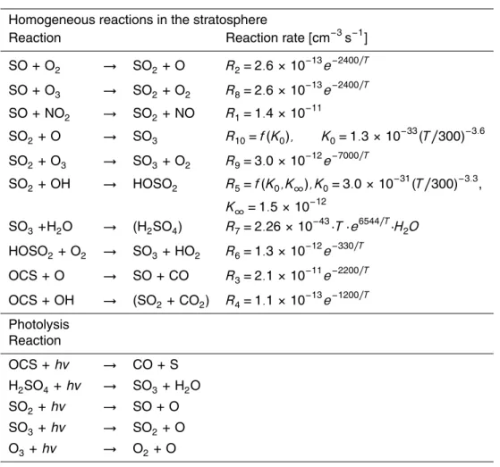
2005). The rate of H₂SO₄ photolysis in the UV range was estimated according Turco et al. (1979) and Rinsland et al. (1995) based on the MESSy calculated photolysis rate of HCl. Treating photolysis rates offline excludes the verification of recently proposed mechanisms of H₂SO₄photolysis by visible light (Vaida et al., 2003; Mills et al., 2005a). Reactions and reaction rates are listed in Table 1.

5

2.4 Observational data

The model is evaluated with satellite-measured integral aerosol quantities, size re-solved in situ aerosol measurements and precursor observations from several cam-paigns. Our analysis focusses on the validation of the aerosol size dependent in-tegral quantities surface area density (SAD), volume density (VD), and effective

ra-10

dius (Reff). The satellite data sets described below may contain other

informa-tion as well, which are not considered here due to their higher retrieval

uncertain-ties. We also do not take into account the SPARC ASAP/CCMVal stratospheric

aerosol climatology (SPARC/ASAP, 2006, http://www.pa.op.dlr.de/CCMVal/Forcings/ CCMVal Forcings WMO2010.html) because the product is only robust for aerosol

sur-15

face densities.

In this paper, integrated aerosol quantities are compared to stratospheric aerosol cli-matologies provided by the University of Oxford (PARTS, 2004; Wurl et al., 2010), here-inafter referred to as UOX, and the NASA AMES Laboratory (Bauman et al., 2003a,b), hereinafter referred to as AMES. The data sets give information about the integrated

20

parameters surface area density, volume density, e_ffective radius, total concentration as well as the size distribution geometric radius and distribution width.

In both data sets aerosol size parameters are retrieved from extinction profiles mea-sured with a sun occultation instrument during the Stratospheric Aerosol and Gas Ex-periments (SAGE) II, aboard the ERBS satellite (McCormick, 1987). The instrument

25

(13)

GMDD

3, 1359–1421, 2010

R. Hommel et al.

Title Page

Tables Figures

◭ ◮

Back Close

Full Screen / Esc

Discussion

P

a

per

|

Dis

cussion

P

a

per

|

Discussion

P

a

per

|

Discussio

n

P

a

per

The AMES climatology considers data from km above the tropopause only. In the UOX solution all extinction profiles were taken into account that passed a quality screening. Thus, the UOX climatology provides data within and potentially below the tropopause. Since the AMES climatology ends in August 1999, our analysis is build upon 1998 data which are seen as representative for the stratospheric background after the volcanic

5

eruption of Mt. Pinatubo in 1991 (Deshler et al., 2006; SPARC/ASAP, 2006).

The AMES climatology combines the four wavelength extinction measurements from SAGEII with extinction profiles at 12.82 µm from the Cryogenic Limb Array Etalon Spec-trometer (CLAES; Roche et al., 1993), which, in particular, has advantages in the de-tection of volcanic aerosol. The algorithm retrieves the effective radius, surface area,

10

volume density, and the width of a unimodal log-normal size distribution by examining satellite-measured extinction ratios to pre-computed values utilising a look-up table in combination with a parameter search technique. As Bauman et al. (2003b) showed, in the volcanically quiescent stratosphere AMES retrieved aerosol surface area is a few percent larger than in the climatology of Thomason et al. (1997) which is based on

15

Principal Component Analysis (PCA; Thomason et al., 1997; Steele et al., 1999). In the UOX climatogy an inversion technique is applied based on the Bayesian Op-timal Estimation (BOE) theory. Details on the method are given in Wurl et al. (2010). The BOE approach combines a priori knowledge of measured particle size distributions (Deshler et al., 2003a) with spectral aerosol extinction measurements. That makes the

20

BOE solution sensitive to fine mode particles which are practically invisible for the spec-tral instrument (Kent et al., 1995; Steele et al., 1999). A further strength of the BOE method are error estimates as part of the retrieval process. In contrast, other inversion techniques like PCA attract solutions with a systematic bias (Steele et al., 1999). Wurl et al. (2010) showed that the BOE method is applicable in the presence of large

ex-25

(14)

GMDD

3, 1359–1421, 2010

R. Hommel et al.

Title Page

Tables Figures

◭ ◮

Back Close

Full Screen / Esc

Discussion

P

a

per

|

Dis

cussion

P

a

per

|

Discussion

P

a

per

|

Discussio

n

P

a

per

|

the different observation techniques (SPARC/ASAP, 2006), this is a clear advantage in improving the quality of globally monitored stratospheric background aerosols.

In situ measurements of aerosol quantities are inferred from optical particle counter (OPC) measurements in the stratosphere over Laramie (Wyoming, 41.3◦N, 105.7◦W). To date the Laramie record is the most coherent in situ observation (see SPARC/ASAP,

5

2006, and references therein). The counter, operative since 1971, measured strato-spheric particle number concentrations at R≥0.15 and 0.25 µm. In 1989 the instru-mentation was redesigned, now being able to resolve aerosol spectra in 12 channels from≥0.15 to 2.0 µm. A condensation nuclei (CN) counter simultaneously measures particles with a radius of 10 nm±10%. Further details on the instrumentation and error

10

estimates of derived aerosol quantities are given in Deshler et al. (2003a).

The modelled abundance of SO2and gaseous H2SO4are compared with data from literature. In addition, the modelled abundances of SO2is compared to measurements taken during the Stratospheric Aerosol and Gas Experiment (SAGE) III Ozone Loss and Validation Experiment (SOLVE), conducted from December 1999 to March 2000

15

(e.g. Lee et al., 2003). SO2was measured by a chemical ionisation mass spectrom-eter (CIMS; Hunton, 2000) onboard the NASA research aircraft DC-8. The detec-tion limit was approximately 25 pptv. The flights were made in the Arctic high lati-tudes and occasionally in the mid-latilati-tudes at altilati-tudes between 9 and 13 km. SOLVE data were obtained from NASA’s ESPO archive (http://espoarchive.nasa.gov/archive).

20

Of the ∼11 000 samples for SO2, approximately only one fifth were made below the tropopause and are not considered in our analysis. The data include samples from the volcanic plume of the Icelandic volcano Hekla, which erupted on 26 February 2000. In the morning of the 28th, the research aircraft passed the plume in a transit flight from Edwards AFB to Kiruna, Sweden, and also several days later volcanic signals are

25

(15)

GMDD

3, 1359–1421, 2010

R. Hommel et al.

Title Page

Tables Figures

◭ ◮

Back Close

Full Screen / Esc

Discussion

P

a

per

|

Dis

cussion

P

a

per

|

Discussion

P

a

per

|

Discussio

n

P

a

per

2.5 Experiment setup

The model was integrated for 17 years, starting in January 1990. To shorten the model’s spin-up period, prognostic aerosol components were initialised from a zon-ally averaged aerosol mass mixing ratio which was derived from the climatological mean volume density of the UOX SAGE II climatology. We assumed the aerosols

5

throughout the stratosphere are homogeneously composed of 75% sulphuric acid with a density of 1.7 g cm−3. The total mixing ratio was distributed to the size sections assuming an unimodal size distribution following Pinnick et al. (1976) with a mode ra-dius of 0.0725 µm and a standard deviation of 1.86. Prognostic sulphate precursors were not initialised. Instead, the atmospheric abundance of DMS, SO₂ and H₂SO₄is

10

formed from boundary layer fluxes during the model integration.

Initialising aerosols rather than synthesise adequate abundances in the stratosphere solely from surface emission fluxes requires an assessment of the model’s prognostic aerosol parameters in respect of their potential drift. We analysed the evolution of each size section’s aerosol mixing ratio and other quantities from the free troposphere

15

(∼350 hPa) to altitudes (∼3 hPa), where sulphuric acid aerosols are no longer ther-modynamically stable due to elevated H2SO4 vapour pressures. Shown in detail in Hommel (2008), we found that all diagnosed parameters are balanced in the sixth year of integration. The following eleven years are the base for our model climatology.

3 Results and discussion

20

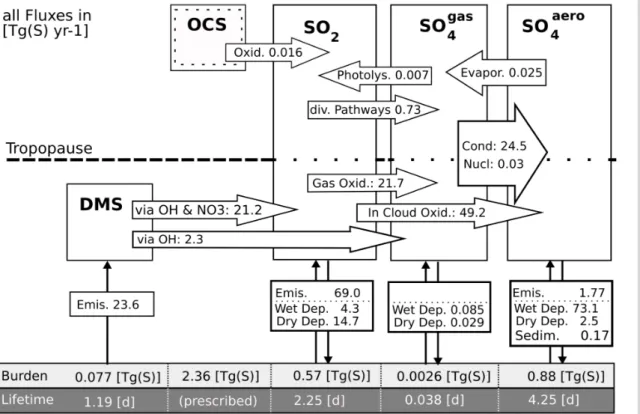
3.1 Global budgets

Figure 1 shows a schematic diagram of the global budget of prognostic sulphur con-stituents based on annual means of the last year of integration. Atmospheric life-times are given as global residence life-times. As noted before, DMS oxidation is con-strained to the troposphere and OCS mixing ratios are prescribed. In the budget

(16)

GMDD

3, 1359–1421, 2010

R. Hommel et al.

Title Page

Tables Figures

◭ ◮

Back Close

Full Screen / Esc

Discussion

P

a

per

|

Dis

cussion

P

a

per

|

Discussion

P

a

per

|

Discussio

n

P

a

per

|

diagnostics special consideration is given to ECHAM5’s standard aerosol module HAM (Stier et al., 2005; Kloster et al., 2006) since both models use identical tropospheric process parametrisations and surface emission flux strengths. Hence, apparent diff er-ences in conversion rates diagnosed from both models are directly attributed to module specific treatments of aerosol dynamics.

5

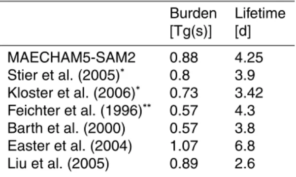
With the explicit consideration of aerosol processes in the stratosphere, both the calculated global mean burden of sulphate aerosol and the lifetime are∼17% larger than in ECHAM5-HAM. Nevertheless the values are in the range of predictions from other global models, where aerosol processes are more or less constrained to the troposphere (Table 2). In the stratosphere Takigawa et al. (2002) diagnose an annual

10

mean burden of sulphate aerosol of 0.149 Tg(S) from the CCSR/NIES aerosol cou-pled middle-atmosphere AGCM. This corresponds well with 0.148 Tg(S) derived in this study (17% of the total aerosol burden). However, the global annual mean burden of sulphate aerosol in Takigawa et al. (2002) with 0.36 Tg(S) is 60% smaller than in our model. Besides a different handling of source strengths, potentially the neglected

15

tropospheric aqueous phase chemistry in the CCSR/NIES model accounts for this dis-tinct discrepancy. It is widely approved that aqueous phase chemistry converts ap-proximately two thirds of the emitted SO2to sulphate (Chin et al., 1996; SPARC/ASAP, 2006), see discussion below. Pitari et al. (2002) model a 2% higher stratospheric aerosol burden (0.151 Tg(S)) in a hybrid AGCM/CTM, resolving the size of sulphate

20

aerosol by a sectional method with 15 bins. They refer to an estimated stratospheric aerosol burden of 0.156 Tg(S) based on SAGE I/SAM II data (Kent and McCormick, 1984) from 2 km above the tropopause for the year 1979, a year in which the strato-sphere was near background after the volcanic eruption of Fuego in 1975. Comprehen-sively diagnosed are prognostic sulphur compounds and their transformation rates in

25

(17)

GMDD

3, 1359–1421, 2010

R. Hommel et al.

Title Page

Tables Figures

◭ ◮

Back Close

Full Screen / Esc

Discussion

P

a

per

|

Dis

cussion

P

a

per

|

Discussion

P

a

per

|

Discussio

n

P

a

per

with lower numbers calculated without additionally imposed fluxes of SO₂and sulphate particles from the troposphere to the stratosphere.

Model predicted deposition rates of sulphur compounds differ not more than 10% from ECHAM5-HAM, except that the flux of sedimenting particles is a factor two weaker in our model. An overestimation of sedimentation rates from modal aerosol modules

5

was also highlighted by Weisenstein et al. (2007) in a 2-D model intercomparison study under stratospheric conditions. The aqueous phase production of sulphate in tropo-spheric clouds is 6% larger than in ECHAM5-HAM and accounts for 65% of the total global sulphate production, which is in the ballpark of other studies (e.g. Pham et al., 1995; Penner et al., 2001; Liu et al., 2005). Relative to the transformation rates of 2-D

10

model AER as shown in SPARC/ASAP (2006), in our simulation the stratospheric SO₂ oxidation is one order of magnitude larger. Differences in the in the three-body reaction oxidising SO2 by the hydroxyl radical OH (see Weisenstein et al., 1997) may explain this relatively large discrepancy between both models.

In altitudes, where H2SO4 is supersaturated, the residence time of sulphuric acid

15

vapour is considerably shorter than that of SO2. In our simulation a three times longer

lifetime of gaseous H₂SO₄ is predicted than diagnosed from ECHAM5-HAM (Stier

et al., 2005; Kloster et al., 2006). This is clearly attributed to the extended vertical rep-resentation of the atmosphere in the AGCM MAECHAM5, because, as shown later in Sect. 3.2, above 30 km (which is the TOA in the in the studies performed with

ECAHM5-20

HAM) the mixing ratio of gaseous H2SO4 is several orders of magnitude larger than below. In our simulation 98% of the global total sulphuric acid vapour condenses onto existing particles, only 0.1% nucleates and the remaining part deposits in the planetary boundary layer. Compared to ECHAM5-HAM, the mass transfer of H2SO4from the gas to the particle phase via new particle formation is 3.6 times weaker in our model. This

25

(18)

GMDD

3, 1359–1421, 2010

R. Hommel et al.

Title Page

Tables Figures

◭ ◮

Back Close

Full Screen / Esc

Discussion

P

a

per

|

Dis

cussion

P

a

per

|

Discussion

P

a

per

|

Discussio

n

P

a

per

|

stratospheric background, however, predicted aerosol size distributions from both mod-ules are almost indistinguishable in the accumulation and coarse mode. Also the size of fine particles (R <0.01 µm) is better represented in SAM2 than in HAM compared to a benchmark model. A potential method to further improve the treatment of the two processes condensation and nucleation, which compete for the available sulphuric acid

5

vapour, is given in Hommel and Graf (2010). In this study it was shown that reserving a certain fraction of the available sulphuric acid vapour for nucleation significantly im-proves the SAM2’s ability to capture particle growth under elevated levels of SO₂in the stratosphere.

Interestingly, the modelled rate of evaporating sulphates in the stratosphere is

al-10

most twice as strong as the oxidation rate of OCS, which is suggested to stabilise stratospheric aerosol abundances above 25 km (SPARC/ASAP, 2006). Depending on its set up, the 2-D model AER predicts OCS oxidation fluxes from 0.032 Tg(S) yr−1

(SPARC/ASAP, 2006) to 0.049 Tg(S) yr−1 (Weisenstein et al., 1997). For the 3-D

CCRS/NIES model Takigawa et al. (2002) diagnose 0.036 Tg(S) yr−1. Our modelled

15

OCS oxidation rate is less than half than in the other models, what seems to be caused by the offline treatment and superimposing of OCS mixing ratios with photolysis rates taken from another model (see also Sect. 3.2).

Photolysis of sulphuric acid vapour above 35 km is a major nonvolcanic pathway

for the SO₂ abundance in the upper stratosphere and mesosphere (discussed in

20

Sect. 3.2). In our study, 7×10−3Tg(S) yr−1 of the gaseous H₂SO₄in the stratosphere is photolysed to SO2. This is 1% of the total SO2 which is oxidised to sulphuric acid vapour above the tropopause.

3.2 Aerosol precursor gases

In this section we compare results of the modelled abundance of the prognostic

sul-25

(19)

GMDD

3, 1359–1421, 2010

R. Hommel et al.

Title Page

Tables Figures

◭ ◮

Back Close

Full Screen / Esc

Discussion

P

a

per

|

Dis

cussion

P

a

per

|

Discussion

P

a

per

|

Discussio

n

P

a

per

and hence approximately negligible (Weisenstein et al., 1997). Prescribed fields are used for OCS.

During several field campaigns sulphur-bearing gases were measured in the tro-posphere, but were measured only sporadically in the stratosphere (reviewed in SPARC/ASAP, 2006). Early in situ observations of SO₂ (Meixner, 1984; M ¨ohler and

5

Arnold, 1992) and sulphuric acid vapour (Arnold and Fabian, 1980; Viggiano and Arnold, 1981; Arnold et al., 1981; Heitmann and Arnold, 1983; Arnold and Qiu, 1984; Schlager and Arnold, 1987; M ¨ohler and Arnold, 1992; Reiner and Arnold, 1997) were conducted in the middle and upper stratosphere of NH mid-latitudes, some of them during volcanically active periods, e.g. the eruption of El Chich ´on in 1982.

Rins-10

land et al. (1995) reported SO₂ profiles in the middle stratosphere provided by the ATMOS infrared spectrometer onboard the NASA Space Shuttle for SPACELAB 3 in 1985. After the massive eruption of the Philippine volcano Mt. Pinatubo in June 1991, a series of flight campaigns measured the abundance of several gases, including SO₂ (SPARC/ASAP, 2006). In contrast to the above mentioned early in situ measurements,

15

both spatial coverage and temporal resolution of nowadays airborne sampling tech-niques increased, but their altitudinal coverage is still often limited to the free tropo-sphere. With respect to newer airborne observations, we choose to validate the

mod-elled abundance of SO2 with previously unpublished measurements made during the

NASA SAGE III Ozone Loss and Validation Experiment (SOLVE), conducted at Arctic

20

high latitudes from December 1999 to March 2000. The majority of the data collected in 14 missions were sampled above the tropopause up to 13 km altitude.

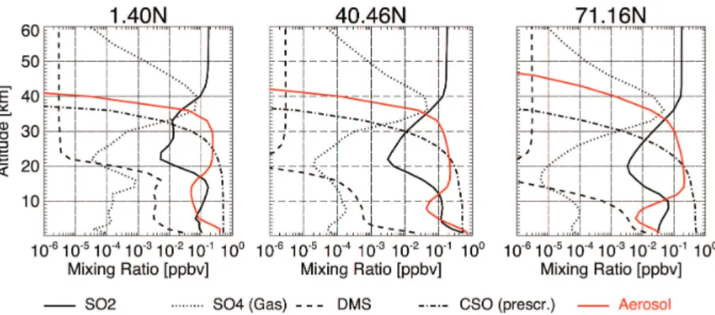
In Fig. 2 a composite of calculated vertical profiles at the equator, the NH mid and high latitudes of all sulphur constituents is shown. In Fig. 3 we compare our model results to other models and specific in situ observations of stratospheric SO2 and

sul-25

(20)

GMDD

3, 1359–1421, 2010

R. Hommel et al.

Title Page

Tables Figures

◭ ◮

Back Close

Full Screen / Esc

Discussion

P

a

per

|

Dis

cussion

P

a

per

|

Discussion

P

a

per

|

Discussio

n

P

a

per

|

transformation of SO₂ to H₂SO₄ and the subsequent partitioning of the latter into aerosol droplets results in the formation of distinct minima in the vertical profiles of both gases, whereas the aerosol mixing ratio increases (Fig. 2). In central and upper regions of the aerosol layer, between 20 and 35 km, photodissociation of OCS increases the stratospheric SO2 abundance. In this region of the stratosphere, the positive gradient

5

of H2SO4 gas mixing ratios is more pronounced than those of SO2. Due to the pos-itive gradient in the stratospheric temperature above the cold point tropopause, both the oxidation rate of SO2and the H2SO4vapour pressure increase with altitude. The latter leads to a with altitude strongly decreasing mass transfer to the particle phase, and more H₂SO₄ is held in the gas phase. When H₂SO₄ is subsaturated aerosols

10

evaporate completely, resulting in a strong negative gradient in the aerosol mixing ra-tios above 30 km (Fig. 2). Between 37 and 40 km, H2SO4released into the gas phase reaches peak mixing ratios of ∼70 pptv. Slightly lower values are found in mid and high latitudes. Above 40 km, sulphuric acid vapour is photolysed to SO₃, which in turn rapidly photolyses to SO2 (Burkholder and McKeen, 1997), ultimately forming a

15

reservoir of SO2in the stratosphere above 40 km.

Measurements by the ATMOS infrared spectrograph onboard the NASA Space Shut-tle for SPACELAB 3, made from April to May 1985 between 26 and 32 N, confirm the formation of such a SO2 reservoir (Fig. 3). However, the data also revealed a nega-tive gradient in the SO₂ mixing ratio around the stratopause (Rinsland et al., 1995).

20

This gradient cannot be reproduced in our experiment. Instead, the SO2 mixing ratio remains approximately constant in heights above 50 km. Whether this is due to an unresolved mechanism in the modelled photochemistry or due to a missing sink in the microphysics, e.g. vapour uptake by meteor debris (e.g. Mills et al., 2005b; Turco et al., 1981), remains speculative since neither of the processes postulated in the literature

25

is confirmed experimentally.

(21)

GMDD

3, 1359–1421, 2010

R. Hommel et al.

Title Page

Tables Figures

◭ ◮

Back Close

Full Screen / Esc

Discussion

P

a

per

|

Dis

cussion

P

a

per

|

Discussion

P

a

per

|

Discussio

n

P

a

per

et al., 2003). However, in our analysis volcanic samples where not excluded from the data, since our statistical analysis revealed that the signal of the UT/LS background concentration of SO2is robust in the data set and showing a well pronounced normal distribution at all altitudes: The median of the measured background concentration in the LS with 35 pptv (0.25 and 0.75 percentiles at 28.3 and 43.3 pptv) is 20% below

5

the analysis of Lee et al. (2003), which excluded data above 200 pptv and considered also samples made in the UT. In Fig. 4, outliers (represented by larger spread of the data as well as mean values lying beyond the interquartile range, IQR, of the data) are clearly marking measurements affected by volcanic SO2. Modelled SO2is more biased relative to SOLVE in the lower latitudes. At 46◦N, between 10 and 11 km,

MAECHAM5-10

SAM2 overpredicts the mixing ratio by 58% in DJF and by 150% in MAM. In higher latitudes most of the model data are at least within the IQR of the observations.

A detailed investigation how sulphate aerosol models predict stratospheric SO2 mix-ing ratios in the tropics and subtropics was given in SPARC/ASAP (2006). With minor exceptions due to the different treatment of chemical and physical processes in the

15

models, the predicted profiles are in qualitative agreement. The spread of the data, however, is rather large between the models. Some of the models are also distinctly biased relative to the ATMOS observations (Rinsland et al., 1995) in the middle and upper stratosphere. As seen in the Figs. 2 and 3 our model does not predict a distinct maximum in the (sub)tropical SO₂ mixing ratio around the 28 km altitude, which was

20

more pronounced in the model results shown in SPARC/ASAP (2006) and Mills et al. (2005a).

For SO₂the Mills et al. (2005a) model clearly underpredicts the ATMOS observations (Fig. 3a) whereas sulphuric acid vapour is within the range of observations above 28 km (Fig. 3b). Below, where aerosol concentrations are largest, Mills et al. (2005a) clearly

25

overpredicts gaseous H₂SO₄by more than 50%. MAECHAM5-SAM2 is in agreement

(22)

GMDD

3, 1359–1421, 2010

R. Hommel et al.

Title Page

Tables Figures

◭ ◮

Back Close

Full Screen / Esc

Discussion

P

a

per

|

Dis

cussion

P

a

per

|

Discussion

P

a

per

|

Discussio

n

P

a

per

|

Vertical profiles of SO₂ in the tropics as predicted by the 2-D model AER (Weisen-stein et al., 1997) exhibit vertical displacements in the altitudes showing maxima and minima compared to our simulation. The displacements prevail in the extratropics and are in the order of−6 km, relative to our data, from above the tropopause to heights of

∼35 km. The profiles for sulphuric acid vapour are in qualitative agreement, in the

trop-5

ics AER shows∼50% larger values than our model but in the NH mid-latitudes the bias is marginal up to 32 km height. The vertical profiles of SO₂are in good agreement to the 3-D Japanese CCRN/NIES model in the tropics and NH mid-latitudes (Takigawa et al., 2002). In our simulation, higher mixing ratios are found in the tropical tropopause layer (TTL), and up to 80% lower SO₂ mixing ratios occur where the stratospheric aerosol

10

abundance is largest (above 20 km). Due to missing links in the chemistry, the Taki-gawa et al. (2002) model does not reproduce the stratospheric reservoir of SO2above 30 km. Their H2SO4 in the gas phase is much lower than in our simulation. The 1-D stratospheric aerosol model of Turco et al. (1979) and Toon et al. (1979) predicted pro-files for SO2and sulphuric acid vapour very similar to those shown in Fig. 2. Differences

15

are seen in the representation of upper stratospheric mixing ratios of SO2, which are up to one order of magnitude larger in our simulation, and of gaseous H₂SO₄, which do not show a distinct negative gradient above 26 km.

A model-intercomparison in SPARC/ASAP (2006) revealed only minor differences between the models regarding the OCS abundance in the atmosphere. Models agree

20

to a large extend with observations made in the stratosphere. Our offline data are based on these published data, and so it is assumed that OCS mixing ratios are well represented in our model.

Despite different representations of stratospheric dynamics in the models mentioned above, 1-D models behave like global models with respect to the representation of the

25

(23)

GMDD

3, 1359–1421, 2010

R. Hommel et al.

Title Page

Tables Figures

◭ ◮

Back Close

Full Screen / Esc

Discussion

P

a

per

|

Dis

cussion

P

a

per

|

Discussion

P

a

per

|

Discussio

n

P

a

per

3.3 Global aerosol distribution

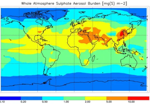
The annual mean burden of modelled sulphate aerosol is shown in Fig. 5. Tropospheric sulphate dominates, since, as analysed in Sect. 3.1, stratospheric aerosol contribute to less than 20% to the global annual mean sulphate mass of the atmosphere. The modelled sulphate burden is in agreement with sulphate components of other model

5

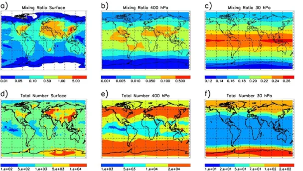
studies which utilise comparable emission scenarios (e.g. Stier et al., 2005; Ma and von Salzen, 2006). Particulate sulphate is concentrated in regions of high anthropogenic sulphur emissions, i.e. industrialised regions in South East Asia, Europe, and Northern America. Significant dispersion of aerosols to Northern Africa and the Middle East occurs in the planetary boundary layer, which is is also seen in aerosol mixing ratios at

10

the surface (Fig. 6a). Zonal homogenisation of the atmosphere’s aerosol abundance increases with altitude (Fig. 6b and c). In the stratosphere (Fig. 6c), the aerosol layer is well stratified and, due to low air density, the mixing ratio in the tropics is approximately as high as in the terrestrial boundary layer. In the free troposphere the mixing ratio of sulphate aerosol is approximately one order of magnitude lower.

15

The annual mean total particle number concentration (NT) is dominated by ultra-fine particles throughout the atmosphere. As in other model studies, e.g. Ma and von Salzen (2006), at the surface the global distribution of the aerosol number concentra-tion is very well correlated with the aerosol mixing ratio. Largest number concentraconcentra-tions are found over continental regions and are associated with anthropogenic pollution.

20

Primary emissions occur mainly in the accumulation mode, thus are less reflected in the total number concentration near the surface (with exceptions in continental regions near the equator) and in the total sulphate aerosol mixing ratio. The global dispersion of

NTin the boundary layer is less pronounced than in the mixing ratios, indicating a rather fast ageing of aerosols, which is associated with a reduction of ultra-fine particle

num-25

(24)

GMDD

3, 1359–1421, 2010

R. Hommel et al.

Title Page

Tables Figures

◭ ◮

Back Close

Full Screen / Esc

Discussion

P

a

per

|

Dis

cussion

P

a

per

|

Discussion

P

a

per

|

Discussio

n

P

a

per

|

relative humidity environments (see Easter et al., 2004; Spracklen et al., 2005; Ma and von Salzen, 2006).

NT increase with altitude, reaching maxima in the mid-latitude free troposphere, where binary homogeneous nucleation rates are largest (Stier et al., 2005; Spracklen et al., 2005; Makkonen et al., 2009). Given the importance of new particle

forma-5

tion for the total particle concentration in the atmosphere, above the boundary layer a pronounced anti-correlation between the total number density and the mixing ratio of sulphate is seen in Fig. 6. This becomes apparent in the stratosphere, where the rates of new particle formation are largest in the spring time polar vortices (see Fig. 7b and c).

10

Figure 7 shows zonal means of the seasonal averaged aerosol mass mixing ratio, nucleation rate, and nucleation mode number density for the 11 year analysis period. The tropical stratospheric reservoir (TSR; Trepte and Hitchman, 1992; Hitchman et al., 1994), a region which is quasi isolated from meridional transport, as well as the iso-lated air masses in the SH polar vortex are clearly seen in the modelled aerosol mixing

15

ratio (Fig. 7a). Distinct staircase patterns found in the subtropical mixing ratio result from interactions between advective transport by the mean meridional circulation, the meridional circulation associated with the quasi-biennial oscillation, the semi-annual oscillation, and effects of isentropic mixing by the absorption of planetary wave energy (Baldwin et al., 2001). In agreement with findings of Hitchman et al. (1994) on the basis

20

of aerosol data from the space-borne SAM and SAGE instruments, a transport regime has been identified in the lower stratosphere, where particles are transported pole-ward and downpole-ward during winter. These patterns persist into subsequent equinoctial seasons and are most pronounced in the NH. The same authors deduced an upper transport regime in the tropics during summer (above 22 km), which is also reflected

25

(25)

GMDD

3, 1359–1421, 2010

R. Hommel et al.

Title Page

Tables Figures

◭ ◮

Back Close

Full Screen / Esc

Discussion

P

a

per

|

Dis

cussion

P

a

per

|

Discussion

P

a

per

|

Discussio

n

P

a

per

There is no evidence from the modelled aerosol mixing ratio isolines that the high abundance of aerosols within the TSR is supplied by sulphate particles of tropospheric origin, transported into the LS by tropical upwelling. Instead, in boreal summer a sig-nificant flux of tropospheric particles reaches the LS in the subtropics and midlati-tudes. The regions, where in our model aerosols are uplifted into the LS correspond

5

to cells of tropospheric convection over the Asian Monsoon/Tibetan Plateau region, which is one of the main pathways for the cross-tropopause transport of atmospheric moisture and other trace gases (see Fueglistaler et al., 2009, and references therein). Aerosols reaching the LS are transported poleward within the lower stratospheric trans-port regime, but a significant amount of particles also reaches the tropics via the upper

10

Monsoon’s anticyclone (Bannister et al., 2004; Fu et al., 2006).

Preferred regions where new sulphate droplets are formed in the model are the free troposphere above 500 hPa as well as the winter and spring time polar vortices above the 70 hPa pressure altitude (Fig. 7b). Within a few kilometres above the tropopause, where temperatures are as low as 200 K, the Vehkam ¨aki parametrisation of binary

ho-15

mogeneous nucleation predicts a minimum in the nucleation rate, which is not seen in studies using the models ECHAM4-SAM (Timmreck, 2001) or AER (Weisenstein et al., 1997). A second maximum in tropical stratospheric nucleation rates is seen be-tween 60 and 50 hPa, leading to remarkably high nucleation mode number densities of<10 cm−3throughout the tropical lower stratosphere, up to the 30 hPa pressure

alti-20

tude. Brock et al. (1995) showed particle mixing ratio profiles from measurements in the tropics in March 1994, when Mt. Pinatubo aerosols declined to near-background levels (the data were attributed as cleared from volcanic aerosol). The profiles exhibit that total number mixing ratios of volatile particles are largest in the free troposphere, but also reveal a minimum directly above the tropopause and a second maximum above,

25

(26)

GMDD

3, 1359–1421, 2010

R. Hommel et al.

Title Page

Tables Figures

◭ ◮

Back Close

Full Screen / Esc

Discussion

P

a

per

|

Dis

cussion

P

a

per

|

Discussion

P

a

per

|

Discussio

n

P

a

per

|

origin contribute to the formation and maintenance of a stable stratospheric aerosol layer also in volcanically quiescent periods. But our calculations also reveal that a significant portion of TSR aerosol might be formed in the tropical LS before it ages in higher altitudes and becomes mixed to the extratropics.

High CN concentrations in the spring time polar vortices are observed in altitudes

5

well above the aerosol layer (reviewed in SPARC/ASAP, 2006). Zhao and Turco (1995) first suggested, using a 1-D model, that the formation of an Antarctic stratospheric CN layer strongly depends on the subsidence of a non-condensable gas like SO₂ in the polar night vortex. Mills et al. (1999) and Mills et al. (2005a) showed that in the upper stratosphere SO2 originates from photolysis of H2SO4 and is transported poleward

10

with the mean meridional circulation. In descending air masses of the Antarctic polar vortex SO2 is rapidly oxidised when sunlight returns in spring, hence it triggers the formation of the polar stratospheric CN layer. Furthermore they showed that, nearly independent on the photochemistry mechanisms, which are thought to account for a stabilised stratospheric reservoir of SO2, new particle formation is likely also in polar

15

winters according to the classical nucleation theory. However, in the southern polar vortex a sharp increase in the CN concentration is not predicted until enough gaseous H2SO4is supplied for condensation in late August.

In our model this formation of polar stratospheric CN layers is reproduced (Fig. 7b). In the Arctic polar vortex nucleation occurs in altitudes between 1 and 10 hPa also in

20

winter, with stronger rates at the end of the season. In March, nucleation rates are of similar strength (not clearly reflected in Fig. 7b due to seasonal averaging), but centred at lower altitudes around 20 hPa. In the Antarctic stratosphere significant nucleation rates are seen at 10 hPa in April and July. When sunlight returns in late August, rates of new particle formation increase to 5×10−3cm−3s−1in descending air masses below

25

(27)

GMDD

3, 1359–1421, 2010

R. Hommel et al.

Title Page

Tables Figures

◭ ◮

Back Close

Full Screen / Esc

Discussion

P

a

per

|

Dis

cussion

P

a

per

|

Discussion

P

a

per

|

Discussio

n

P

a

per

In Antarctica MAECHAM5-SAM2 predicts peak CN concentrations slightly higher than observed. However, location, subsidence as well as depletion of the CN layer corre-spond well with CN counter observations by e.g. Hofmann et al. (1989).

Meridional transport of stratospheric aerosols is not restricted to the motion of air masses relative to the mean meridional circulation of the stratosphere. From Fig. 7c,

5

an efficient lateral mixing of ultra-fine particles from the polar vortices into stratospheric mid and low latitudes due to Rossby wave activity (e.g. Waugh et al., 1994) can be deduced. There is evidence for a stronger wave activity in the NH since in the middle stratosphere gradients in number density appear stronger than in the SH. Although no nucleation occurs in those regions of the stratosphere, ultra-fine particles mixed to

10

mid-latitudes are growing to larger sizes or even evaporate, dependent on the partial and vapour pressure of H2SO4(Fig. 8).

The upper branch of the stratospheric aerosol layer is not only a region where aerosols shrink in size due to the release of sulphuric acid and water into the gas phase (Fig. 8). Here the model predicted climatologies of the zonal mean H2SO4vapour

pres-15

sure as well as the concentration of sulphuric acid vapour, which is transferred from the gas to the particle phase (condensation) and vice versa (evaporation), are shown. The ability of sulphuric acid vapour to condense onto preexisting particles is strongly re-duced at the cold tropopause. In the lower stratosphere, from a few kilometres above the tropopause to regions where sulphate aerosol evaporates, the mass transfer onto

20

the particles remains remarkably constant. This region corresponds to the central region of the aerosol layer. The non-existence of meridional gradients in the mass transfer concentration of H₂SO₄condensation implies that, at least in the stratospheric background, condensational growth is approximately constant over broad regions of the aerosol layer. Consequently, one may assume that the shape of particle size

dis-25

(28)

GMDD

3, 1359–1421, 2010

R. Hommel et al.

Title Page

Tables Figures

◭ ◮

Back Close

Full Screen / Esc

Discussion

P

a

per

|

Dis

cussion

P

a

per

|

Discussion

P

a

per

|

Discussio

n

P

a

per

|

to H₂SO₄condensation and growth due to coagulation does not change significantly at all latitudes in this region (except in high latitudes near 30 hPa, where small particles evaporate quickly). When the nucleation rate increases, coagulation becomes a more effective sink for aerosols withR <0.07 µm.

In the mid latitudes, at altitudes where sulphate droplet evaporation is largest

5

(Fig. 8c) also an enhanced H2SO4 vapour condensation is found (Fig. 8b). Breaking waves in the “Surf Zone” (McIntyre and Palmer, 1984) yield fluctuations in the strato-spheric temperature, which in turn changes the direction of H2SO4mass transfer onto or offthe particle phase. Such fluctuations last a couple of days. In the averaged clima-tologies of Fig. 8b and c, regions of vapour condensation above 20 hPa overlap with

re-10

gions where aerosols evaporate. Thereby H₂SO₄condensation stabilises stratospheric aerosols until the particles are further transported poleward, where vapour pressures are higher and where they ultimately evaporate.

Detailed investigations of the interannual variability of the modelled stratospheric aerosol layer, in particular on interactions with the quasi-biennial oscillation, are given

15

in a companion paper (Hommel et al., 2010).

3.4 Stratospheric aerosol climatology

In this section, the model climatology of integrated aerosol quantities is compared with data retrieved from the spaceborne SAGE II instrument. The integral of the model results is taken for particles exceeding 50 nm in radius in order to achieve comparability

20

with detection limitations of optical instruments (Dubovik et al., 2000; Pitari et al., 2002; Thomason et al., 2008; Kokkola et al., 2009).

From Fig. 9 it can be seen that relative to SAGE II higher moments of the aerosol distribution are better represented in the model than lower moments. The variability of the satellite retrieved second and third moments of the aerosol distribution (SAD and

25