Progressive Planar Acoustic Waves: Do Fish Otoliths
Rock?
Petr Krysl1*, Anthony D. Hawkins2, Carl Schilt3, Ted W. Cranford4
1University of California San Diego, La Jolla, California, United States of America,2Loughine Ltd, Kincraig Blairs, Aberdeen, United Kingdom,3Bigleaf Science Services, North Bonneville, Washington, United States of America,4Quantitative Morphology Consulting, Inc., San Diego, California, United States of America
Abstract
Fish can sense a wide variety of sounds by means of the otolith organs of the inner ear. Among the incompletely understood components of this process are the patterns of movement of the otoliths vis-a`-vis fish head or whole-body movement. How complex are the motions? How does the otolith organ respond to sounds from different directions and frequencies? In the present work we examine the responses of a dense rigid scatterer (representing the otolith) suspended in an acoustic fluid to low-frequency planar progressive acoustic waves. A simple mechanical model, which predicts both translational and angular oscillation, is formulated. The responses of simple shapes (sphere and hemisphere) are analyzed with an acoustic finite element model. The hemispherical scatterer is found to oscillate both in the direction of the propagation of the progressive waves and also in the plane of the wavefront as a result of angular motion. The models predict that this characteristic will be shared by other irregularly-shaped scatterers, including fish otoliths, which could provide the fish hearing mechanisms with an additional component of oscillation and therefore one more source of acoustical cues.
Citation:Krysl P, Hawkins AD, Schilt C, Cranford TW (2012) Angular Oscillation of Solid Scatterers in Response to Progressive Planar Acoustic Waves: Do Fish Otoliths Rock? PLoS ONE 7(8): e42591. doi:10.1371/journal.pone.0042591
Editor:Christof Markus Aegerter, University of Zurich, Switzerland
ReceivedApril 14, 2012;AcceptedJuly 10, 2012;PublishedAugust 9, 2012
Copyright:ß2012 Krysl et al. This is an open-access article distributed under the terms of the Creative Commons Attribution License, which permits unrestricted use, distribution, and reproduction in any medium, provided the original author and source are credited.
Funding:The research was funded by the Office of Naval research, grant number N00014-09-1-0611. The funders had no role in study design, data collection and analysis, decision to publish, or preparation of the manuscript.
Competing Interests:The authors have the following interests. Professor A D Hawkins is the Managing Director of Loughine Ltd, a company principally engaged in research activities. The company has a policy of publishing its work. Carl Schilt is owner and sole proprietor of Bigleaf Science Services in North Bonneville, Washington, USA. Bigleaf Science Services is a one-person company which, in cooperation with colleagues, publishes its work. Dr. Ted Cranford is the owner and sole proprietor of Quantitative Morphology Consulting, Inc., USA. Quantitative Morphology Consulting, Inc. is a company which, in cooperation with colleagues, publishes its work. There are no patents, products in development or marketed products to declare. This does not alter the authors9adherence to all the PLoS ONE policies on sharing data and materials, as detailed online in the guide for authors.
* E-mail: [email protected]
Introduction
Fish can sense and respond to a wide variety of sounds. They use sounds to communicate with one another, detect prey and predators, navigate from one place to another, avoid hazards, and analyse the world around them (see Ref. [1] for a recent review). The means by which fish detect sounds involve the otolith organs of the inner ear and are relatively well understood. Sound detection mechanisms in fish have been comprehensively reviewed by Popper et al [2]. However, elucidating the way these organs analyse sound quality and in particular how they enable fish to discriminate between sounds from different directions has proved more difficult.
The motion of the otolith organs of the white seabass (Atractoscion nobilis), a species of croaker, was studied in [3] using a finite element model of the three pairs of otoliths embedded in a viscoelastic matrix (tissue) and exposed to pressure waves in water [4]. The model otoliths were observed to execute both linear translation and angular oscillation, which we have called ‘‘rocking’’. Subsequently we decided to use similar modeling tools to examine whether the angular motion was also to be observed in rigid scatterers in water as opposed to in an elastic matrix. An experimental study was also initiated in parallel by an independent
research team [5]. The present work describes the model of the motion of rigid scatterers in acoustic fluids in response to progressive harmonic waves. The motivation for this work derives from the possibility that the angular motion of the otoliths may be an additional acoustical cue that the fish may use to process sounds.
The traditional view for sound detection proposes that fish tissue has similar acoustic properties (in terms of density and elasticity) to the surrounding water. When the fish is moved back and forth by a sound field, the dense otoliths within the ear lag behind because of their inertia, thereby creating shearing forces at sensory hair cells [6,7]. Each hair cell is directional in its response to mechanical stimulation [7,8].
are inherently sensitive to the kinetic sound component, particle velocity or its time derivatives particle acceleration or particle displacement, and not sound pressure [13,14].
There is an issue over the determination of the direction of a sound source by fish. The ability of fish to discriminate sounds from different directions is clear, but the mechanism by which they achieve this has yet to be elucidated (see review in Ref. [15]). It has been established that teleost fish are able to discriminate between spatially separated sources under far-field conditions, both in the horizontal [16–18] and vertical [19] planes. Indeed, they are able to distinguish between sound sources at different distances [20]. This ability not only enables fish to locate the sources of sound but may also assist them in discriminating sounds from a particular source against the general non-directional noise background.
How then do fish determine the direction of a sound source? One of the obstacles in the way of understanding the mechanisms for determining sound direction is our lack of knowledge of the patterns of movement of the otoliths themselves. Is the simple two-dimensional accelerometer model proposed by de Vries [9,10] adequate to explain the motion of the otolith, or are the movements more complex? How does the otolith organ respond to sounds from different directions? Sand and Michelson [21] examined the motion of different parts of the saccular otolith of the European perch (Perca fluviatilis). Using a tray attached to a horizontal shaker to hold the preparation and a laser vibrometer to detect otolith motions. They observed that vibration of the fish in the horizontal plane along its long axis resulted in vertical movements of both ends of the otoliths at several driving frequencies. An area of minimum vertical movement appeared around the midpoint of the otolith at different frequencies, indicating the existence of a horizontal axis of rotation or rocking. The results suggested a frequency dependent pattern of otolith rotational movement as a result of linear horizontal translation.
In the present work we attempt to understand variability in the motion of the otolith by studying the response of dense rigid scatterers suspended in an acoustic fluid to acoustic planar progressive waves. This problem was studied for the sphere by Hickling and Wang [22]. Both steady-state forces and torques exerted on elastic objects were studied by Smith [23], but the resulting motion was not addressed. This aspect was further investigated by Olsson [24], with the limitation that time-harmonic excitation was considered for spheroidal objects, but even though the possibility of angular oscillation was accounted for in the model it was not studied. Also, multiple scattering and multiple scatterers were not accommodated in the model. Fan et al. [25] studied acoustic (steady-state) radiation torques on arbitrary scatterers, but the resulting motion was not analyzed.
In this work we present an approach that allows us to study the motion of rigid scatterers suspended in an acoustic fluid in response to acoustic incident long-wavelength planar progressive waves and (multiple) scattered waves. First, in Section 2, we formulate a qualitative mechanical model for the motion of such scatterers. The model predicts that the motion will include both translational and angular oscillation, provided the scatterer is sufficiently asymmetric. In Section 3, we detail an acoustic time-domain finite element model. Verification of the model is undertaken in Section 4 where we report simulations of the response of a spherical scatterer for which the reference solution exists. The model is validated in Section 5 using recent experiments of Rodgers [5]. The hemispherical scatterer is found to oscillate both in the direction of the progressive waves and also in the plane of the waves as a result of angular oscillatory motion. Finally, in Section 6 we describe some numerical experiments that illustrate the rocking motion phenomena. Importantly, our model
predicts that a rocking motion will be displayed by all irregularly shaped scatterers including fish otoliths. It is therefore possible that hearing mechanisms in fish could make use of this additional component of oscillation.
Methods
Qualitative Model of Motion
1.1 Setting and assumptions. Consider a progressive planar harmonic wave in an acoustic fluid (in this paper we are mostly concerned with water) with mass densityr, speed of soundc, and angular frequencyv. The acoustic wave impinges upon a stiff (so stiff that it may be considered rigid) homogeneous scatterer of arbitrary shape, whose characteristic dimensions aare all much smaller than the wavelength of the incident acoustic wave (it is ‘‘acoustically small’’)
avvl~2pc
v : ð1Þ
Expressed in the terms of the wavenumber k~2p=l, this assumption readskavv1. In particular, for an otolith in water
we havea&5mmandl&3000mm(for a 500 Hz signal), and the assumption is quite adequate.
Without any loss of generality, we will assume that the pressure is described in Cartesian coordinates such that the incident plane wave front is orthogonal to the X axis, and the center of the Cartesian coordinates is at the center of gravity of the scatterer. As a consequence of the assumption (11) the incident pressure, the scattered pressure, and their sum, the total pressure, around the scatterer at any time may be approximated by a Taylor series in coordinates X,Y,Z. To a first approximation we will limit the Taylor series to include only the constant and linear terms. For the pressure around the scatterer we write
p(X,Y,Z,t)~AzbXzcYzdZ ð2Þ where all the coefficients of the Taylor series are functions of time, A~A(t), and so on. We will symbolically refer to the coefficients of the Taylor series asA,b,c,dand distinguish their meaning by explicitly specifying whether the expansion is for the incident pressure or the total pressure.
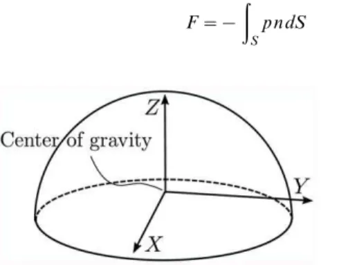
1.2 Resultant force. Henceforth we omit the time argument, with the understanding that the force changes in time. The force exerted upon the scatterer by the pressure in the surrounding fluid can be evaluated at any time as
F~{
ð
S
p n dS ð3Þ
whereSis the surface of the scatterer, andnis the outer normal to the surface. We will writep(X,Y,Z,t)andn(X,Y,Z,t)only when confusion is possible; otherwise the arguments will be omitted. The time-dependent force F causes the scatterer to accelerate in response to the forcing by the pressure according to Newton’s equation.
Substituting (2) into (3) we obtain the forceFin the form of
F~{A
ð
S
n dS{b
ð
S
X n dS{c
ð
S
Y n dS{d
ð
S
Z n dS, ð4Þ
where we may now introduce a particular shape of the scatterer surface to evaluate the individual integrals.
Resultant Torque
The torque exerted upon the scatterer by the pressure in the fluid surrounding it can be evaluated at any time as
T~{
ð
S
r|p n dS ð5Þ
where r~X eXzY eYzZ eZ is the location where the pressure
acts on the surface of the scatterer, and eX,eY,eZare unit basis
vectors of the Cartesian coordinates. Equation (5) may be rewritten using the expansion of the cross product as
T~{eXÐ
SðYnZ{ZnYÞp dS
{eY Ð
SðZnX{XnZÞp dS
{eZ Ð
SðYnX{XnYÞp dS:
ð6Þ
Upon substitution of (2) the individual integrals read
Ð
SðYpnZ{ZpnYÞdS~ A Ð
SðYnZ{ZnYÞdS
zbÐ
SðYXnZ{ZXnYÞdS
zcÐ
SðYYnZ{ZYnYÞdS
zdÐ
SðYZnZ{ZZnYÞdS ð7Þ
and
Ð
SðZpnX{XpnZÞdS~ A Ð
SðZnX{XnZÞdS
zbÐ
SðZXnX{XXnZÞdS
zcÐ
SðZYnX{XYnZÞdS
zdÐ
SðZZnX{XZnZÞdS ð8Þ
and finally
Ð
SðYpnX{XpnYÞdS~ A
Ð
SðYnX{XnYÞdS zbÐ
SðYXnX{XXnYÞdS zcÐ
SðYYnX{XYnYÞdS zdÐ
SðYZnX{XZnYÞdS
ð9Þ
Total Response Decomposition
The total pressure is composed of the incident pressure and the scattered pressure. Consequently, we may evaluate the total response of the scatterers as a superposition of the response due to the incident pressure and the response due to the scattered pressure. We will now apply this principle to the calculation of the dynamic force and torque acting on the solid scatterer.
First we consider the effect of the uniform incident pressure. It is readily demonstrated that the first integral on the right of (4) due to uniform pressure does not contribute to the force no matter what the shape of the surface of the scatterer. We can write
ð
S
n dS~eX ð
S
nXdSzeY ð
S
nYdSzeZ ð
S
nZdS: ð10Þ
Consider a surface element dS. According to the well-known tetrahedron argument [26], we have the relationship between the projection of the elementary surface area into the planeX~0
dSX~nXdS ð11Þ
and similarly for the other two coordinate planesY~0andZ~0
dSY~nYdS, dSZ~nZdS: ð12Þ
Now, because the surface S is closed, each elementary surface (dS)z
may be paired with another elementary surface(dS){
such that(dS)z
and(dS){
project into the same-size area in the plane X~0
D(dSX) z
D~D(dSX) {
D ð13Þ
and the components of the normals to the corresponding elementary surfaces have opposite signs
(nX) z:
(nX) {
v0: ð14Þ
Analogous arguments can be made for projections into the coordinate planesY~0and Z~0. Since these observations are true for all elementary surfaces dS, the contributions to the integrals from all such pairs will cancel and we have
ð
S
nXdS~0, ð
S
nYdS~0, ð
S
nZdS~0 ð15Þ
and consequently
ð
S
n dS~0: ð16Þ
This finding demonstrates the conclusion that uniform pressure in the acoustic fluid would not accelerate the embedded scatterer.
F~{bÐ
SX n dS~{b eX Ð
SXnXdS
zeY Ð
SXnYdSzeZ Ð
SXnZdS
ð17Þ
Similar arguments as above for the uniform pressure term can be applied. For instance,
ð
S
XnYdS~0 ð18Þ
because for any pair of elementary surfaces such that (nYdS)z~{(nYdS){ the corresponding coordinate X is the
same for both, and we again get cancellation among all the pairs. Equation (17) for the force that acts on a spherical scatterer therefore reduces to
F~{b
ð
S
X n dS~{beX ð
S
XnXdS, ð19Þ
where the integral is evaluated over the surface of the sphere. The result
Figure 2. Perturbation (scattered) pressure distribution around the hemispherical scatterer at a particular time instant.The scatterer is the void in the middle. Planar incident wave ofkR~0:07. The pressure amplitude is coded by shade, the darker the shade the higher the positive (red) or negative (blue) pressure. Level curves of pressure are also shown.
doi:10.1371/journal.pone.0042591.g002
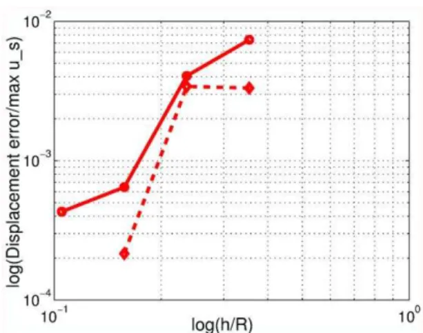
Figure 3. Approximate error of the normalized displacement amplitude for the spherical scatterer.
ð
S
XnXdS~ 4 3pR
3 ð20Þ
reproduces the observation that for acoustically small spheres (see equation (1)) the accelerating force will be proportional to the product of the average pressure gradient (b) and the volume of the sphere.
The dynamic torque for a spherical scatterer is always zero, under all conditions, not only for the incident pressure, but also for the total pressure, as all the elementary pressure forces pass through the center of the sphere (the center of gravity).
Hemispherical Scatterer, Response to Incident Pressure Now consider a hemispherical scatterer of radiusR shown in Figure 1. Note that the center of gravity of the hemisphere is at a distance of38Rfrom the center of the spherical surface. Only the coordinate planeY~0is a plane of symmetry for the pressure on the scatterer surfaceS. The Taylor series expansion of the incident pressure will contain no contribution of the linear term in theY direction, c~0, and no contribution of the linear term in theZ direction,d~0. The force will be therefore evaluated as
F~{bÐ
SXn(X,Y,Z)dS~
{b eX Ð
SXnXdS
zeYÐSXnYdSzeZÐSXnZdS ð21Þ
A similar argument as above for the uniform pressure term can be applied. Hence, we conclude that the accelerating force on the hemispherical scatterer will be in the form
F~{beX ð
S
XnXdS ð22Þ
Therefore the scatterer will be accelerated by the incident pressure into oscillation only in the direction of the wave propagation. The integral evaluates to
ð
S
XnXdS~ 2 3pR
3, ð23Þ
and again this finding is in agreement with the observation that the
Figure 4. Mesh of the hemispherical scatterer located in the tank. Mesh size of 2 mm on the surface of the scatterer. doi:10.1371/journal.pone.0042591.g004
Figure 5. Approximate error (dashed line) and estimated true error of the longitudinal displacement of the hemispherical scatterer for the finite element solutions for excitation frequency of 100 Hz.
accelerating force will be proportional to the product of the average pressure gradient and the volume of the scatterer.
We shall now evaluate the dynamic torque due to the incident pressure on a hemispherical scatterer with the Cartesian coordi-nates origin located at the center of gravity (Figure 1). All of the integrals that define the torque components for the linearly varying incident pressure (2) in the immediate vicinity of the scatterer can be shown to be identically zero. This follows from the Gauss-Ostrogradski theorem
Ð
SQnXdS~ Ð
V
LQ
LXdV, Ð
SQnYdS~ Ð
V
LQ
LYdV, Ð
SQnZdS~ Ð
V
LQ
LZdV,
ð24Þ
where upon substitution of a quadratic expression in the coordinates with the origin at the center of gravity, for instance Q~XZ, we find
ð
S
QnXdS~ ð
S
XZnXdS~ ð
V
LQ LXdV~
ð
V
ZdV: ð25Þ
The rightmost integral is the definition of the static moment with respect to the planeZ~0. Recall thatX,Y,Zare Cartesian axes at the center of gravity, and all such static moments are by definition zero. For the same expression we also obtain
ð
S
QnYdS~ ð
S
XZnYdS~ ð
V
LQ LYdV~
ð
V
0dV~0 ð26Þ
and
ð
S
QnZdS~ ð
S
XZnZdS~ ð
V
LQ LZdV~
ð
V
XdV ð27Þ
which is identically zero by the same static-moment argument. All other combinations are investigated analogously. Therefore, this argument shows that to first-order the incident pressure does not produce any dynamic torque on a scatterer of arbitrary shape.
Hemispherical Scatterer, Response to Scattered Pressure The scattered pressure distribution is not known analytically. As shown by theoretical argument (for instance in [27]) for low frequencies (smallka) the scattered (perturbation) pressure will be similar to that generated by a translating object in fluid, and hence dipole-like. See Figure 2 for an illustration of the perturbation pressure as computed numerically for a hemispherical scatterer. Note this is just a snapshot from a time-dependent process. For any direction in the planeX,Ythis picture would be similar as the scatterer is axially symmetric with respect to the axis Z. The pressure distribution would evidently change if the symmetry was broken such as for the sound fronts being oriented arbitrarily with respect toX,Y,Z.
In the first approximation we may take a distribution of the scattered pressure that varies along the surfaceSas the projection of the translation due to the incident pressure along theXaxis onto the outer normal to the surfaceS
p(X,Y,Z,t)~y(t)nX(X,Y,Z): ð28Þ
The torque components due to this scattered pressure distribution are
TX~y ð
S
YnXnZ{ZnXnY
ð ÞdS~0 ð29Þ
and
TY~y ð
S
ZnXnX{XnXnZ
ð ÞdS~{ypR
3
4 ð30Þ
and finally
TZ~y ð
S
YnXnX{XnXnY
ð ÞdS~0: ð31Þ
Clearly, the scattered pressure generates a nonzero dynamic torque about theY axis. Therefore we conclude that our simple model predicts harmonic rocking (wobbling) of rigid scatterers in incident planar harmonic sound waves. In the following sections we will illustrate this point with a numerical investigation using the finite element method.
Finite Element Model
The equation for the acoustic pressure
1
c2€pp{div(gradp)~0 ð32Þ is treated with the Galerkin approach to yield the weighted residual equation
Table 1.Comparison of simulations with experiments [5].
Quantity
Frequency
[Hz] Experiment Model
Longitudinal displacement [mm] 100 3.33 2.98
200 0.61 0.57
Rocking/longitudinal displacement ratio
100 7.5% 12.8%
200 9.8% 12.8%
Hemisphere.
doi:10.1371/journal.pone.0042591.t001
Table 2.Comparison of simulations with experiments [5].
Quantity
Frequency
[Hz] Experiment Model
Longitudinal displacement [mm] 100 3.38 3.08
200 0.62 0.59
Rocking/longitudinal displacement ratio
100 9.5% 8.8%
200 9.4% 8.8%
ð
V
g1 c2€pp dVz
ð
V
(gradg) gradp dV~
ð
S2
gLp
Ln dS: ð33Þ
HereS2is part of the boundary of the volumeVwhere the normal component of the pressure gradient is prescribed, andgis the test function which vanishes on the part of the boundaryS1where the pressure is prescribed.
The total pressure p is decomposed into the pressure of the known incident wave pinc and the unknown perturbation (scattered) pressure P as p~pinczP, and the appropriate boundary conditions for the constituent parts are formulated next. The problem is solved in a volume of acoustic fluid Vof finite extent. The computational volumeVencloses the scatterer. First we consider a rigid simply-connected scatterer of mass densityrs, volume Vt, and surface S2,t. The surface of the computational
domain is divided into the part where the fluid is adjacent to the enclosed rigid scattererS2,tand the part where the fluid inside the
computational domain is separated from the infinite extent of fluid exterior to the computational domainS2,o.
On the surface of the rigid body scattererS2,tthetotalpressurep
satisfies the boundary condition
Lp
Ln~{rvv_n~{ran, ð34Þ whereanis the acceleration of the surface of the scatterer in the
direction of the outer normal to the fluid surface n due to the motion of the scatterer. This may be expressed in terms of the acceleration of the center of gravity of the scattererA, and the angular acceleration of the scatterer about its center of gravitya
an(r)~n:ðA{~rraÞ: ð35Þ
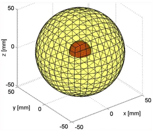
Hereris the position vector of a given point on the surface of the scatterer relative to its center of gravity, and ~rr is the skew-Figure 6. Simulation of hemispherical scatterer.Illustration of the mesh with 8 element edges per radius on the surface of the domain; the surface of the scatterer is shown in solid (red) color, and the outer surface with the absorbing boundary condition is transparent (yellow). doi:10.1371/journal.pone.0042591.g006
Table 3.Hemisphere in infinite fluid medium.
Quantity Frequency [Hz] Model
Longitudinal displacement [mm] 100 3.184
200 0.598
Rocking/longitudinal displacement ratio 100 13.4%
200 13.4%
doi:10.1371/journal.pone.0042591.t003
Table 4.Hemicylinder of 4 inch length in infinite fluid medium.
Quantity Frequency [Hz] Model
Longitudinal displacement [mm] 100 3.389
200 0.643
Rocking/longitudinal displacement ratio 100 14.8%
200 14.8%
symmetric matrix used to express a vector cross product
~rr~
0 {rz ry
rz 0 {rx
{ry rx 0
2
6 4
3
7
5: ð36Þ
The weighted residual equation boundary term on the surface of the scatter therefore reads
ð
S2,t
gLp LndS~{
ð
S2,t
grn:ðA{~rraÞdS: ð37Þ
On the surface S2,o where the fluid extent is truncated the
boundary conditions are applied separately to the incident pressure and the perturbation pressure. For the incident pressure the pressure gradient is known. For instance, for a planar harmonic wave we have
pinc~pAsinð{k:xzvtÞ ð38Þ
and therefore the gradient of the incident pressure onS2,oreads
Lpinc
Ln ~{pAcosð{k:xzvtÞ(k:n): ð39Þ Absorbing (radiation) boundary condition is applied to the perturbation pressure. The simplest such boundary condition is the early-time plane wave approximation
LP Ln~{
1
c LP
Lt~{
1
cPP_ ð40Þ
for the perturbation pressure onS2,o, and that was found sufficient
for the present application: the convergence rate is apparently affected but remains satisfactory.
The weighted residual statement is written with the above boundary conditions as
ð
V
g1 c2PP dV€ z
ð
S2,o
g1 cPP dS_ z
ð
V
(gradg) gradP dV
z
ð
S2,t
grn dS:Az
ð
S2,t
grn:ð{~rrÞdS:a
~ {
ð
V
g1
c2€ppincdV{ ð
V
(gradg) gradpincdV
z
ð
S2,o
gLpinc Ln dS:
ð41Þ
To eliminate the translational and angular acceleration of the scatterer we invoke Newton’s equation: acceleration A may be written in terms of the mass of the scattererM~ÐV
trsdV and force applied on its surface
A~M{1F , ð42Þ
where the force applied on the scattererFis produced by the total pressure on the surface of the scatterer
F~
ð
S2,t
(Pzpinc)nT dS: ð43Þ
Here n is the outer normal to the fluid-scatterer boundary with respect to the solid. Similarly the angular acceleration of the scatter about its center of gravity may be written in terms of its tensor of inertia and the applied torque
a~I{1T , ð44Þ
where the torque applied on the scattererF is produced by the total pressure on the surface of the scatterer
T~
ð
S2,t
~rr:(Pzpinc)nTdS: ð45Þ
Here the tensor of inertia is
I~
ð
Vt
rs~rrT:~rr dV: ð46Þ
Substituting for the accelerations from (42) and (44) into (41) results in a weighted residual equation for the perturbation pressure as the only unknown. Classical finite element discretiza-tion (with iso-parametric hexahedra, or tetrahedra, in the present case) allows us to write the matrix equations for a system of ordinary differential equations for the nodal pressures
½S½PP€z½D½PP_zð½Cz½HÞ½P~½Linc: ð47Þ
Here ½Sis the acoustic stiffness matrix,½Dis the absorbing-boundary condition damping matrix, ½C is the acoustic mass matrix, and½His defined as
½H~r½GFTM {1½G
Fzr½GTT½I {1½
GT, ð48Þ
where the coupling matrices½GFand½GTimplement the discrete
form of (42) and (44)
½A~M{1½F~M{1½G
F ½ðPz½pincÞ, ½a~½I{1
½T~½I{1
½GT ½ðPz½pincÞ:
ð49Þ
The load vector consists of.
½Linc~{½S½€ppinc{ð½Cz½HÞ½pincz½Lo,inc, ð50Þ
where½Lo,incis the matrix expression of the incident-pressure load term onS2,o. Using the definition
allows us to rewrite (47) as a system of coupled first order differential equations
½PP_~½Q
½S½QQ_z½D½Qz½C_½P~½Linc
: ð52Þ
Straightforward discretization in time with the trapezoidal rule yields
½P1~½P0zDt
2 ½Q0z½Q1
½S½Q1~½S½Q0{½DDt
2 ½Q0z½Q1
{½C_Dt
2 ½P0z½P1
zDt
2 ½Linc0z½Linc1
, ð53Þ
which results in the time-stepping algorithm: (a) solve for perturbation pressure rate
2
Dt½Sz½Dz Dt
2½C _
½Q1~
2
Dt½S{½D{ Dt
2½C _
½Q0{½C_2½P0
z ½Linc0z½Linc1
ð54Þ
then (b) update perturbation pressure
½P1~½P0zDt
2 ½Q0z½Q1
, ð55Þ
and finally (c) evaluate the accelerations from (49) and integrate to obtain velocities and displacements. To address the possibility of the presence of multiple scatterers we may realize that the above argument applies separately to each of the scatterers, with the understanding that the perturbation pressure Paccounts for the presence of all scatterers. Therefore the computation is straight-forward and the only additional effort involves the construction of the multiple coupling matrices ½H and the update of the accelerations for each scatterer. This computational scheme was implemented in the Matlab toolkit FAESOR [26].
Results
1. Verification
The response of a movable spherical scatterer was studied in detail by Hickling and Wang [22]. The amplitude of the displacement in the direction of the progressive wave is predicted by their equation (5), with the displacement function given for the large wavelength limit in equation (3) of the above reference. Here we predict the motion of the spherical scatterer with the finite element model described above. The computational domain was a sphere of water 15 mm in radius (bulk modulus k~2100MPa, mass densityr~1000kg:m{3). The spherical scatterer with radius of 5 mm of mass densityr~2500kg:m{3 was embedded in the center of the domain. The finite element mesh was structured, and composed of eight-node hexahedra.
The scatterer was initially at rest, and the progressive planar harmonic waves in the positiveXdirection, with incident pressure amplitude of 1 kPa, were introduced with frequency of 100 Hz. The model was also exercised with other (long-wavelength) frequencies, without significant difference in the match between the analytical and numerical predictions. The computed dynamic response was post-processed to extract the amplitude of the steady-state motion of the sphere.
TheXdisplacement (in the direction of the progressive wave) of the center of gravity is normalized by the displacementmaxuS
computed for a spherical scatterer in [22]
maxuS~DpincD
vrc
3
2rs=rz1: ð56Þ
The computed results are used to define the approximate error of the displacement amplitude as
Figure 7. Approximate error (dashed line) and estimated true error of the longitudinal displacement of the hemispherical scatterer for the finite element solutions for excitation frequency of 100 Hz.
doi:10.1371/journal.pone.0042591.g007
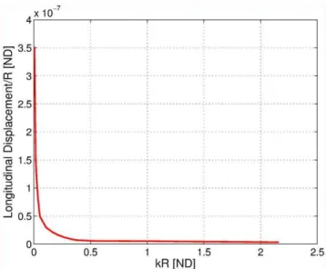
Figure 8. Longitudinal displacement normalized by the radius of a hemisphere scatterer as a function of frequency (in terms of the parameterkR).
Eu,hj~
uhjz1{uhj
maxuS
: ð57Þ
Figure 3 demonstrates the convergence of the finite element approximation. The normalized displacement amplitude was computed for four meshes, with two, four, eight, 16 element edges per radius as 0:95412,0:98831,0:99998 and 1:0033. The log-log plot of the approximate errors shows satisfactory conver-gence rate of approximately 1.7, and the finest mesh renders the motion amplitude within 1% error.
Validation
An experimental study to detect and quantify the angular motion of rigid scatterers in water was recently reported [5]. Aluminum scatterers were suspended submerged in a cylindrical tank with piston-generated standing waves (this rig approximated the conditions of an unsuspended scatterer in infinite medium). The longitudinal and angular oscillatory motion was measured with a variety of techniques. While the experimental study [5] was ongoing we were supplying the experimenters with blind predictions. Here we reproduce the results for the hemispherical scatterer and for one hemicylinder configuration.
In the simulations, the sound speed of water was taken as c~1500m=s, and mass density as r~1000kg:m{3. The hemi-spherical aluminum scatterer with radius ofR~0:5in&12:7mm and the hemicylinder aluminum scatterer with radius of R~0:5in&12:7mm and length L~4:0in&101:6mm, of mass densityrs~2700kg:m{3, were suspended at the depth of 70(i. e. 177.8 mm, halfway between the piston and the free surface) in the cylindrical tank.
The excitation signals of 200 Hz and a pressure amplitude of 738.2 Pa, which corresponds to the experimental measurement of 261 Pa RMS at 7 inch depth, and of 100 Hz and a pressure amplitude of 973.0 Pa, which corresponds to the experimental measurement of 344 Pa RMS at 7 inch depth, were considered.
1.1 Hemispherical scatterer. Unstructured graded (four-node) tetrahedral meshes with mesh size on the surface of the
scatterer of 1.33, 2.0, 3.0, and 4.5 mm were used. One such mesh is shown in Figure 4 where the surface of the hemispherical scatterer is enclosed within the transparent surface of the volume of the water.
The four finite element solutions for the displacement and angular rotation were used in a Richardson’s extrapolation procedure [26] to extract the limit values. For the longitudinal displacement (in the direction of the propagation of the wave) two successive solutions yielded the normalized approximate error as
Eu,j~
ujz1{uj maxus
ð58Þ
where maxus is the displacement amplitude of an equivalent
spherical scatterer from [22], anduj,j~1,2,3 are the numerical
solutions. The true error was then estimated from the relation (12.17) of [26]
Eu(hj)~(1{ab) {1E
u,j ð59Þ
whereEu(hj)was the true error for mesh sizehj,a~2=3was the
refinement factor, andbwas the rate of convergence, which had to be estimated theoretically as the data was not sufficiently smooth for a reliable least-squares estimate of the convergence rate (as shown in Figure 5). In this instance, we assumedb~1:0due to the use of the first order absorbing boundary condition.
The computed amplitude of total displacement in the direction of the wave propagation (longitudinal) and rocking displacement (amplitude of displacement perpendicularly to the flat base of the scatterer) is reported in Table 1. The predicted longitudinal displacement for both excitation frequencies can be seen to be quite close to the experimental measurements. The agreement of the ratio of the rocking/longitudinal displacement is, for reasons incompletely understood at this point, not as good. Perhaps the suspension of the hemispherical scatterer somehow prevented the transverse displacement to some degree.
Hemi-cylindrical Scatterer
Three lengths 499, 699, and 899respectively, of hemi-cylindrical rods were tested [5]. For the sake of brevity we report comparison for just the 499configuration. The same material properties and pressure gradients as for the hemispherical scatterer were assumed. Similar approach to the limit procedure as for the hemispherical scatterer was adopted to produce results reported in Table 2. The agreement of the longitudinal displacement and of the ratio of the rocking/longitudinal displacement for both excitation frequencies can be seen to be quite good.
Hemispherical Scatterer in Infinite Medium
The experimental rig aims to produce conditions similar to a free-floating scatterer in infinite acoustic medium. In the previous sections we reported simulations that emulate the actual boundary conditions of the cylindrical tank with a piston at the bottom and a free surface of the top. Here we report simulations for scatterers placed in an infinite extent of acoustic fluid. First for the hemispherical scatterer, and then for the hemicylindrical scatterer. The computational domain was a sphere of water of the radius mRwith absorbing boundary condition, where m needed to be chosen judiciously to reduce the effect of the boundary of the domain on the solution. It was determined by experimentation that taking the volume of water to be a sphere of radius four times the radius of the scatterer (m~4) reduced the boundary effect to the fourth significant digit.
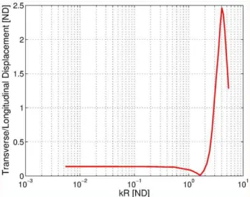
Figure 9. Ratio of transverse to longitudinal displacement of a hemisphere scatterer as a function of frequency (in terms of the parameterkR).
Hexahedral meshes with 9, 14, and 20 edges per radius were used. The meshes were structured and therefore the mesh size increased with distance from the surface of the scatterer: Compare with a sample mesh in Figure 6. The hemispherical scatterer’s surface is shown in solid color, and the outer spherical surface on which the absorbing boundary conditions are applied is shown transparent.
The excitation signal of the incident planar wave was considered at 200 Hz with a pressure amplitude of 2.478 kPa (corresponding to experimental measurement of 261 Pa RMS at 7 inch depth), and at 100 Hz and a pressure amplitude of 6.532 kPa (corresponding to experimental measurement of 344 Pa RMS at 7 inch depth).
The computed total displacement in the direction of the wave propagation (longitudinal) and rocking displacement (perpendic-ularly to the flat base of the scatterer) is reported in Table 3. The rocking to longitudinal displacement ratio is rather larger than for the tank configuration.
Hemicylinder Scatterer in Infinite Medium
For the sake of brevity we report comparison for just the 499
long cylinder configuration. The same material properties and pressure gradients as for the hemispherical scatterer were used. The domain was an elongated ellipsoid that enclosed the scatterer with water of approximately the thickness of the diameter of the cylinder. The finite element model used an unstructured tetrahedral mesh (four-node elements). The extrapolated values of displacement computed from results for mesh size of 6.7, 4.5, and 3 mm are reported in Table 4 and the approximate and estimated true error of the longitudinal displacement are displayed in Figure 7. The predicted rocking motions are larger than those measured in the tank. This discrepancy is likely due to the difference of perturbation pressure distribution (which drives the rocking as opposed to the longitudinal motion driven by the incident field) between the free-space and the distribution in the experimental chamber of the finite-size cylinder.
Rocking Experiments
Importantly, the present numerical formulation is not limited to large wavelengths, and that gives us an opportunity to investigate rocking as a function of frequency. For this investigation the computational domain was a sphere of water 15 mm in radius (bulk modulusk~2100MPa, mass densityr~1000kg:m{3). The hemispherical scatterer with radius of 5 mm and mass density rs~2500kg:m{3 was embedded approximately in the center of
the domain. The finite element mesh was structured, and composed of eight-node hexahedra.
The scatterer was initially at rest, and quickly (over a couple of periods) yielded to the excitation by the progressive planar harmonic waves in the positiveXdirection, with incident pressure amplitude of 1 kPa. The incident wave was applied with various frequencies (between 100 Hz and 100 kHz). The longitudinal displacement and the ratio of the transverse and longitudinal displacement were computed as in the previous section.
Figure 8 shows the change of the longitudinal displacement as a function of the wave number (frequency). The displacement can be seen to vary essentially smoothly as an inverse function of the wave number.
Figure 9 shows how the ratio of the transverse rocking displacement to the longitudinal displacement changes as the frequency was increased from low (very-long wavelength) to high
(wavelength commensurate with the radius of the hemisphere). For low frequencies (large wavelengths) the transverse/longitudinal ratio was essentially independent of the frequency of excitation. A plausible explanation is that in this frequency range the perturbation pressure distribution does not substantially change, and its amplitude is proportional to the amplitude of the incident wave. For frequencies commensurate with the radius of the scatterer the rocking motion amplitude first seems to pass through a null at around kR~p=2 (i.e. R=l~1=4), to subsequently increase to approximately a double of the longitudinal amplitude.
Discussion
The present results indicate that the motion of complicated shapes such as otoliths under plane harmonic wave excitation is more complex than a simple back-and-forth oscillation in the direction of the progressive waves suggested by Pumphrey [6] and de Vries [9,10]. A simple back and forth translation in the direction of the sound wave would only be the case for a uniform spherical otolith. If the shape of the otolith is irregular and asymmetrical, as it usually is, then motion is also induced in other directions. The rocking (or wobbling) motion may produce additional stimuli that the fish may be able to process for additional cues on the characteristics and direction of the oncoming sound.
For a simple hemisphere the rocking or wobbling motion is significant in magnitude (exceeding 10% of the back and forth oscillation). We might expect it to be much greater for some other shapes. In addition it is conceivable that the suspension system of the otolith in live intact fish may serve to accentuate the rocking motion. Certainly these possibilitites are worthy of further study.
There are more insights to be gained from the present simple models. For instance, how does the excitation direction relative to the orientation of the scatterer or otolith change the response? How does the response depend on the shape of the otolith? How do responses change for a grouping of otoliths (two or more), and how do the resulting motions depend on the excitation direction relative to the arrangement of the scatterers? There are many intriguing questions that may be amenable to closer examination with our models. In particular, the present finite element model can provide answers for multiple scatterers in arbitrary arrange-ments and allows for the actual otolith shapes to be modeled.
We must also not forget that the movements of otoliths are constrained within the otic capsule. Each otolith is surrounded by a fluid, the endolymph, and contained within a capsule. The otolith is attached to the wall of the capsule and placed in close contact with the hair cells of the sensory maculae by an otolithic membrane. These surrounding structures may also restrict and otherwise affect the motion of the otoliths in a way which we hope to investigate further.
Acknowledgments
Discussions with P. H. Rogers of Georgia Institute of Technology pointed the way on numerous occasions.
Author Contributions
References
1. Webb J, Popper A, Fay R, editors (2008) Fish Bioacoustics: Springer. 2. Popper AN, Fay RR, Platt C, Sand O (2003) Sound detection mechanisms and
capabilities of teleost fishes. In: Collin SP, Marshall NJ, editors. Sensory Processing in Aquatic Environments. New York: Springer-Verlag. 3–38. 3. Carl R Schilt, Ted W Cranford, Petr Krysl, Hawkins AD (2011) Vibration of
otolithlike scatterers due to low frequency harmonic wave excitation in water. J Acoust Soc Am 129: 2472–2472.
4. Krysl P, Cranford TW, Hildebrand JA (2008) Lagrangian finite element treatment of transient vibration/acoustics of biosolids immersed in fluids. Int J Numer Meth Engng 74: 754–775.
5. Rodgers G (2011) An Experimental Study in Acoustically Induced Vibration of a Fish Otolith. Georgia: Georgia Institute of Technology. 59 p.
6. Pumphrey R. Hearing; 1950; unknown. Symp. Soc. Exp. Biol. 1–18. 7. Flock A (1965) Electron microscopic and electrophysiological studies on the
lateral line canal organ. Acta Otolaryngol Suppl 199: 1–90.
8. Hudspeth AJ, Corey D (1977) Sensitivity, polarity, and conductance of vertebrate hair cells to controlled mechanical stimuli. Proc Natl Acad Sci USA 74: 2407–2411.
9. DeVries HL (1950) The mechanics of the labyrinth otoliths. Acta Oto-Laryngologica 38: 262–273.
10. DeVries HL (1956) Physical aspects of the sense organs. Prog Biophys Chem 6: 207–264.
11. Sand O, Karlsen H (2000) Detection of sound and linear acceleration in fishes. Philos Trans R Soc Lond 355: 1295–1298.
12. Sand O, Karlsen HE, Knudsen FR (2008) Comment on ‘‘Silent research vessels are not quiet’’. J Acoust Soc Am 121.
13. Chapman C, Sand O (1974) Field studies in two species of flatfish, Pleuronectes platessa (L.) and Limanda limanda (L.) (Family Pleuronectidae) Comp Biochem Physiol: 371–385.
14. Hawkins A, MacLennan D (1976) An acoustic tank for hearing studies on fish. In: Schuijf A, Hawkins A, editors. Sound Reception in Fish. Amsterdam Elsevier. 149–170.
15. Sand O, Bleckmann H (2008) Orientation to Auditory and Lateral Line Systems. Fish Bioacoustics. New York: Springer. 183–231.
16. Schuijf A, Baretta J, Wildschut J (1972) A field investigation on the discrimination of sound direction in Labrus berggylta (Pices: perciformes). Neth Journ Zool 22 81–104.
17. Chapman C, Johnstone A (1974) Some auditory discrimination experiments on marine fish. J exp Biol 61: 521–528.
18. Schuijf A, Buwalda R (1975) On the mechanism of directional hearing in the cod (Gadus morhua). J Comp Physiol 98: 333–343.
19. Hawkins A, Sand O (1977) Directional hearing in the median vertical plane by the cod. J Comp Physiol 122: 1–8.
20. Schuijf A, Hawkins A (1983) Acoustic distance discrimination in the cod. Nature 302: 143–144.
21. Sand O, Michelson A (1978) Vibration measurements of the perch saccular otolith. Comp Physiol 123: 85–89.
22. Hickling R, Wang NM (1966) Scattering of sound by a rigid movable sphere. Journal of the Acoustical Society of America 39 276ff.
23. Smith WE (1972) Acoustic radiation pressure forces and torques from elastic-scattering. Australian Journal of Physics 25 275ff.
24. Olsson P (1985) Acoustic scattering by a rigid movable body immersed in a fluid. Journal of the Acoustical Society of America 78 2132–2138.
25. Fan ZW, Mei DQ, Yang KJ, Chen ZC (2008) Acoustic radiation torque on an irregularly shaped scatterer in an arbitrary sound field. Journal of the Acoustical Society of America 124 2727–2732.
26. Krysl P (2011) Thermal and Stress Analysis with the Finite Element Method. San Diego: Pressure Cooker Press. 389 p.

![Table 1. Comparison of simulations with experiments [5].](https://thumb-eu.123doks.com/thumbv2/123dok_br/18381336.356431/6.918.479.832.117.267/table-comparison-of-simulations-with-experiments.webp)