Marine substrate response from the analysis of seismic attributes in
CHIRP sub-bottom profiles
This paper presents an evaluation of the response of
seismic relection attributes in diferent types of marine
substrate (rock, shallow gas, sediments) using sealoor
samples for ground-truth statistical comparisons.
The data analyzed include seismic relection proiles
collected using two CHIRP subbottom proilers
(Edgetech Model 3100 SB-216S), with frequency
ranging between 2 and 16 kHz, and a number (38) of
sediment samples collected from the sealoor. The
statistical method used to discriminate between diferent
substratum responses was the non-parametric
Kruskal-Wallis analysis, carried out in two steps: 1) comparison
of Seismic Attributes between diferent marine
substrates (unconsolidated sediments, rock and shallow
gas); 2) comparison of Seismic Attributes between
diferent sediment classes in sealoors characterized
by unconsolidated sediments (subdivided according
to sorting). These analyses suggest that
amplitude-related attributes were efective in discriminating
between sediment and gassy/rocky substratum, but did
not diferentiate between rocks and shallow gas. On
the other hand, the Instantaneous Frequency attribute
was efective in diferentiating sediments, rocks and
shallow gas, with sediment showing higher frequency
range, rock an intermediate range, and shallow gas
the lowest response. Regarding grain-size classes and
sorting, statistical analysis discriminated between two
distinct groups of samples, the SVFS (silt and very ine
sand) and the SFMC (ine, medium and coarse sand)
groups. Using a Spearman coeicient, it was found
that the Instantaneous Amplitude was more eicient
in distinguishing between the two groups. None of the
attributes was able to distinguish between the closest
grain size classes such as those of silt and very ine sand.
AbstrAct
Larissa Felicidade Werkhauser Demarco
1*, Antonio Henrique da Fontoura Klein
2, Jorge Antonio
Guimarães de Souza
3Descriptors:
CHIRP, Seismic attributes, Shallow
seismic.
O presente trabalho tem por objetivo apresentar
uma avaliação da resposta dos atributos sísmicos
(Amplitude Instantânea, Amplitude RMS, Energia
e Frequência Instantânea) em diferentes tipos
de substratos marinhos, correlacionando-os com
características sedimentológicas das amostras
coletadas. Foram analisados peris sísmicos obtidos
com um perilador de subsuperfície com sinal do
tipo CHIRP modelo SB-216S da marca EdgeTech,
com frequência de trabalho de 2 e 16 kHz. O método
se deu a partir da análise estatística não-paramétrica
de Kruskal-Wallis foi aplicada para comparar o
comportamento dos atributos com as diferentes
classes dos grãos das amostras (subagrupadas
segundo o grau de seleção) e com diferentes feições.
Com base na análise dos resultados, foi possível
distinguir dois grupos distintos nas amostras, o
grupo SAMF (silte e areia muito ina) e o grupo
AFMG (areia ina, areia média e areia grossa). Como
conclusão, pode-se dizer que os atributos não foram
capazes de distinguir entre as classes mais próximas
dos grãos. Utilizando o coeiciente de Spearman foi
veriicado que o atributo "Amplitude Instantânea"
mostrou-se mais eiciente em separar os dois
conjuntos. Comparando sedimentos, gás e rocha, os
atributos que utilizaram o atributo "amplitude" foram
eicazes em separar os sedimentos do gás e da rocha,
porém não os distinguiram entre as duas feições,
visto que elas apresentaram amplitudes muito altas,
mas semelhantes entre si. O atributo "Frequência
Instantânea" mostrou-se eicaz na diferenciação
entre sedimento, rocha e gás, o sedimento apresentou
uma maior banda de frequência, a rocha uma faixa
intermediária e o gás a menor delas.
resumo
Descritores:
CHIRP, Atributos sísmicos, Sísmica
rasa.
http://dx.doi.org/10.1590/S1679-87592017124306503 1 Instituto de Pesquisas Tecnológicas do Estado de São Paulo
(Av. Prof. Almeida Prado 532 Cid. Universitária - Butantã, São Paulo, SP, 05508-901. Brazil) 2 Universidade Federal de Santa Catarina, Laboratório de Oceanograia Costeira
(Campus Reitor João David Ferreira Lima, s/n - Trindade, Florianópolis, SC, 88040-900. Brazil) 3 CB&I
(Rodovia José Carlos Daux 8600 Sala 102, Bloco 3, Florianópolis, SC, 88050-000. Brazil)
*Corresponding author: [email protected]
INTRODUCTION
The geophysical methods applied to the solid Earth consist of indirect investigations of the subsurface of our Planet to infer the physical properties of the rocks (JONES, 1999). Using seismic relection proiles it is possible to obtain information on the substrata, such as the thickness and internal geometries of the layers, the presence of faults and fractures, as well as the accumulation of shallow biogenic gas and the presence of landslide deposits (AYRES, 2000).
The study of sediments involves the analysis of a number of properties, which is essential to deine their acoustic behavior. The main features and properties sensitive to the acoustic (seismic) behavior of the sedimentary rocks are: grain size, morphology and roundness of grains, texture, porosity, packing, and permeability of the whole rock (DIAS, 2004; JACKSON, 2007).
An important parameter for the acoustic characterization of strata is the acoustic impedance, i.e., the product of sound speed and density (JACKSON, 2007). More speciically, the acoustic impedance contrasts between two strata is proportional to the amount of energy relected at their interface. Sediment densities and velocities depend on their mineralogy, porosity and water content, and these properties can be highly variable within a wide range of values (AYRES, 2000).
The acoustic response will vary according to interaction and combination of sediment properties; each sediment sample produces a diferent acoustic response, so the acoustic wave’s behavior is diferent for each substrate (FALCÃO; AYRES, 2010). As stated by DAMUTH (1978), an eco-character can be classiied using the diferent responses and characteristics of the acoustic signal. The sea loor’s sedimentary nature will determine the behavior of the relected sound wave as a function of the transmission and relection coeicients (appearance of the primary relector), and these can be used to deine an eco-character.
An echo-character can be deined as a set of return signal characteristics. Analyzing the existence of relectors, seismic facies (thickness, roughness, continuity), presence of difraction hyperbolas, acoustic signal penetration, is a tool which can theoretically be used to discriminate between diferent types of eco-character
associated with distinct sealoor types (DAMUTH, 1975). In this way, each type of sediment sample or substrate interacts diferently with the seismic wave evidencing diferent characteristics, and thus a diferent eco-character. Combining this analysis with the use of seismic attributes (i.e., Instantaneous Amplitude and Frequency) can further improve the accuracy of the bottom classiication.
Seismic Attributes include all the information obtained from seismic data by direct measurement, experiment or logical reasoning (TANER, 2001). The analysis of Seismic Attributes as part of seismic relection proile interpretation has been used since the 1920s (CHOPRA; MARFURT, 2005) and their evolution and proliferation are closely related to the development and advance of computer technology, as in the digitization of records and introduction of color scales. The same authors also noted that seismic attributes can be considered a good tool for visualization, classiication, identiication and interpretation of seismic records.
In this paper was chosen CHEN and SIDNEY’s (1997) classiication. This autors considered two broad categories of Seismic Attributes, those that use a speciic time window (RMS amplitude and energy) and the “instantaneous” ones (Instantaneous Amplitude and Frequency).
The RMS amplitude attribute may be described as a type of average relectivity in a speciic time window. This attribute is linked to characteristics of a layer lying between two interfaces (TANER, 2001).
The Energy attribute is generally used to analyze amplitude anomalies in layers of interest (CHEN; SIDNEY, 1997).
The aim of this paper was to test the potential of Seismic Attributes evaluated in marine seismic relection data (Amplitude RMS, Instantaneous Amplitude, Energy, and Instantaneous Frequency) in diferentiating substrates with diferent sediment types (38 collected samples were used during statistical analyses) using a CHIRP-SBP as seismic source.
MATERIAL AND METHODS
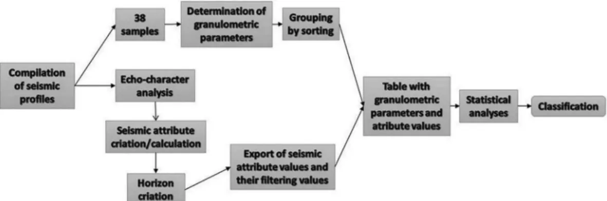
The methodology consisted of 3 parts: 1) the granulometric parameters were determined for the samples collected; 2) the seismic proiles were analyzed, and 3) the seismic attributes were calculated from these proiles. After the creation of the attributes it was necessary to delimit a horizon (to trace a line at the interface between the sealoor and the water) at the seismic proiles (already containing the respective seismic attribute). After the delimitation of the horizons the 3D form was derived from them, because they could thus be exported in a .xyz ile which contained the coordinates and the values of the attribute. This .xyz ile was converted into a table and the particle size parameters were added to it. The statistical analyses were undertaken on the basis of this table. Figure 1 presents a short description of the steps taken during the undertaking of the study.
CHIRP signal
The data were obtained using two Edgetech sub-bottom proilers, models 3100 216S and 3200 SB-512I. Model 3100 has 3 frequency bands within a range of 2-16 kHz. Seismic proiles with a shallow gas feature were obtained with model 3200 SB-512I - with a frequency range between 0.5 and 12 kHz. The CHIRP signal is generated by the stimulation of piezoelectric crystals and received by hydrophones mounted on the vehicle which also carries the acoustic source (MCGEE, 1995).
Distribution of samples
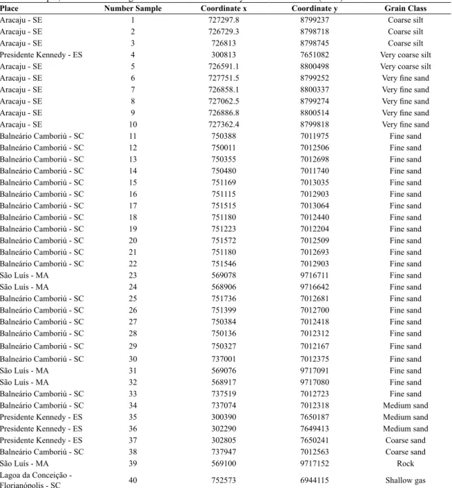
Sediment and rock samples were provided by the CB&I company and the Coastal Oceanography Laboratory (LOC) of the Federal University of Santa Catarina; the locations are along the Brazilian coast, ofshore of ive cities in four states (Figure 2). Seismic lines were selected on the basis of the location of available sediment and rock samples. The description of the sediment samples was made using FOLK and WARD’s (1957) classiication and the granulometric parameters according to the Moments Method proposed by BLOTT and PYE, 2001 (Table 1 and Figure 3).
Attribute evaluation
To calculate seismic attributes from the available data, the open source software OpendTect 4.6.0. was used.
RMS amplitude is deined as the square root
of the arithmetic mean of the squares of the values (LANDMARK, 2004).
where N is the number of interval samples and A is the
amplitude value.
Energy attribute is the square of the sum of the
sample values within a speciic time window divided by the total number of samples in the set time interval. The Energy Attribute is obtained using the following formula (LANDMARK, 2004):
where N is the number of interval samples and A is the
amplitude value.
According to TANER et al. (1979), the complex seismic trace is composed of two parts: a real and an imaginary one. The imaginary component is calculated
( )
RMS
nAi
1
i n 1 2
1
=
=
/
( )
Energy
N
A
12A
22A
n22
=
+
+
using the Hilbert transform. By undertaking this procedure it is possible to separate amplitude and phase, and derive Instantaneous Frequency from phase. Equation (3) shows the result of the complex trace analysis, indicating the instantaneous amplitude and phase.
where A (t) is the Instantaneous Amplitude and θ (t) is
the Instantaneous Phase.
Instantaneous Amplitude can be calculated using
equation 4.
A (t) indicates the Instantaneous Amplitude, f 2(t) the real trace, and f * 2(t) the quadrature trace.
Instantaneous Frequency can be calculated from the
instantaneous phase attribute, illustrated by equations 5 and 6.
where θ (t) indicates the Instantaneous Phase and ω (t)
gives the Instantaneous Frequency.
( )
( )
( )
F t
=
A t e
ji( )t3
( )
( )
( )
( )
A t
=
f t
2+
f
*2t
4
( )
( )
( )
( )
tan
t
f t
f t
5
*1
i
=
-#
&
( )
( )
( )
( )
tan
d
d
t
t
f t
f t
6
*1
~
=
-#
&
Figure 2. Distribution of the samples and the seismic lines. On the left side is the Brazilian coast, on the right are a, Aracaju city, b, São Luis city,
c, the Balneário Camboriu and Florianópolis cities, d, Presidente Kennedy city.
Horizons
After the calculation of the attributes, it is necessary to draw a horizon (2D) on the seismic proile and then derive the 3D horizons from it. Only a 3D horizon can be transfered to the.xyz ile, this ile being necessary for the statistical analyses and comparisons.
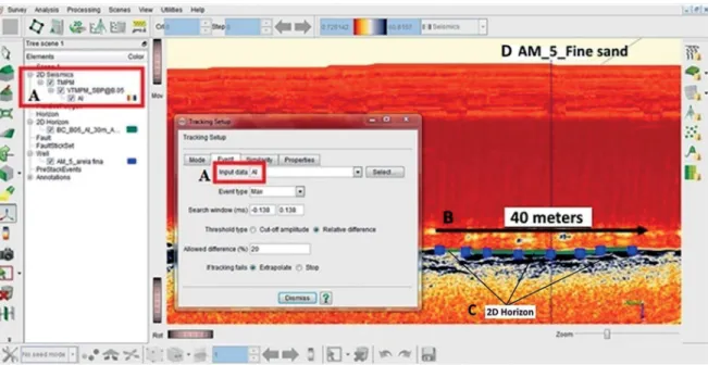
For this step it was necessary to choose the respective attribute for the seismic proile and add the samples collected to it (the seismic proile containing the previously calculated attribute) and draw a horizon at a distance of 15-20 meters on each side of the sample (Figure 4), respecting the relection’s strength, geometry and proile information indicating the corresponding eco-character. The 2D horizon was marked at the interface between sealoor and water, including the proiles with shallow gas.
The conversion from the 2D to the 3D horizon was undertaken using the Extension algorithm. This 3D horizon was transfered to the .xyz ile and the ile converted into a table containing coordinates and attribute values for each seismic line analyzed with each seismic attribute. The attribute values of these tables (this table?) were iltered and outliers excluded. A moving average ilter (applied every 4 or 5 values) was also applied to remove unwanted noise (ROSA, 2010). This inal table was used for the statistical analyses.
Statistical Analysis
Table 1. Sample, rock and shallow gas coordinates. Grain class by FOLK and WARD (1957). Datum WGS 1984.
Place Number Sample Coordinate x Coordinate y Grain Class
Aracaju - SE 1 727297.8 8799237 Coarse silt
Aracaju - SE 2 726729.3 8798718 Coarse silt
Aracaju - SE 3 726813 8798745 Coarse silt
Presidente Kennedy - ES 4 300813 7651082 Very coarse silt
Aracaju - SE 5 726591.1 8800498 Very coarse silt
Aracaju - SE 6 727751.5 8799252 Very ine sand
Aracaju - SE 7 726858.1 8800337 Very ine sand
Aracaju - SE 8 727062.5 8799274 Very ine sand
Aracaju - SE 9 726886.8 8800514 Very ine sand
Aracaju - SE 10 727362.4 8799818 Very ine sand
Balneário Camboriú - SC 11 750388 7011975 Fine sand Balneário Camboriú - SC 12 750011 7012506 Fine sand Balneário Camboriú - SC 13 750355 7012698 Fine sand Balneário Camboriú - SC 14 750480 7011740 Fine sand Balneário Camboriú - SC 15 751169 7013035 Fine sand Balneário Camboriú - SC 16 751115 7012903 Fine sand Balneário Camboriú - SC 17 751515 7013064 Fine sand Balneário Camboriú - SC 18 751180 7012440 Fine sand Balneário Camboriú - SC 19 751223 7012204 Fine sand Balneário Camboriú - SC 20 751572 7012509 Fine sand Balneário Camboriú - SC 21 751180 7012693 Fine sand Balneário Camboriú - SC 22 751546 7012903 Fine sand
São Luís - MA 23 569078 9716711 Fine sand
São Luís - MA 24 568906 9716642 Fine sand
Balneário Camboriú - SC 25 751736 7012681 Fine sand Balneário Camboriú - SC 26 751399 7012700 Fine sand Balneário Camboriú - SC 27 750384 7012418 Fine sand Balneário Camboriú - SC 28 750136 7012312 Fine sand Balneário Camboriú - SC 29 750327 7012167 Fine sand Balneário Camboriú - SC 30 737001 7012375 Fine sand
São Luís - MA 31 569076 9717091 Fine sand
São Luís - MA 32 568917 9717080 Fine sand
Balneário Camboriú - SC 33 737519 7012723 Fine sand Balneário Camboriú - SC 34 737074 7012318 Medium sand Presidente Kennedy - ES 35 300390 7650187 Medium sand Presidente Kennedy - ES 36 302290 7649413 Medium sand Presidente Kennedy - ES 37 302805 7650241 Coarse sand Balneário Camboriú - SC 38 737947 7012563 Coarse sand
São Luís - MA 39 569100 9717152 Rock
Lagoa da Conceição -
Florianópolis - SC 40 752573 6944115 Shallow gas
calculated using the GRADISAT (BLOT; PYE, 2001) by the Moments Method and according to the textural classiication proposed by FOLK and WARD (1957).
The normality test of Shapiro-Wilk W (SHAPIRO; WILK, 1965) was applied to the Seismic Attributes values. The result of this analysis deined the statistical method, whether parametric or nonparametric, to be used in the table containing attribute values, grain classes sub-grouped by sorting. Due to the non-normality of the sample distribution, the lack of homogeneity of the attribute values, and the relatively small
number of samples (38), a non-parametric statistical analysis, using the Kruskal-Wallis method, was chosen.
Figure 4. Example of seismic proile in A, the seismic attribute selected (in this case the Amplitude Instantaneous attribute); in B, the length of the
2D horizon; in C, the 2D horizon; in D, the sample of this proile.
Figure 3. Geometric method of moments. Adapted from BLOTT and PYE (2001).
when there are more than three independent groups to be compared (SIEGEL, 1956), where the independent variables are grain classes (sub-grouped by sorting) and the dependent variable is an attribute value.
A correlation test, comparing attribute values (amplitude and frequency attributes) and mean PHI was applied to calculate the signiicance of each attribute related to grain size. The correlation was performed using the Spearman coeicient, by which values near 0 indicate minimum correlation.
RESULTS
Table 2 shows the sedimentological parameters determined for each sample. In general, the collected samples are poorly sorted and asymmetry and kurtosis
are varied. The samples were obtained from diferent locations (with diferent types of environment), near to and far from the coast, within port areas, and from environments characterized by diferent sedimentary covers and hydrodynamic regimes - which factors alter the samples’ particle size characteristics.
Table 2. Results of granulometric analysis. NS indicates Number of Sample, SD standard deviation, SKE skewness, KUR kurtosis, CS Coarse silt, VCS very coarse silt, VFS Very ine sand, FS ine sand, MS Medium sand and CSS Coarse Sand.
NS Class SD Sorting SKE
Value SKE
KUR
Value KUR
Mean PHI 1 CS 1.80 Poorly sorted -0.23 Symmetrical 1.19 Very platykurtic 5.85 2 CS 1.77 Poorly sorted 0.05 Symmetrical 2.67 Mesokurtic 5.04 3 CS 1.80 Poorly sorted -0.34 Symmetrical 1.19 Very platykurtic 5.96 4 VCS 1.55 Very poorly sorted 0.92 Symmetrical 2.63 Mesokurtic 4.42 5 VCS 1.69 Poorly sorted 0.93 Fine skewed 2.48 Platykurtic 4.55 6 VFS 1.85 Poorly sorted -0.16 Very coarse skewed 5.03 Leptokurtic 3.91 7 VFS 0.36 Well sorted 0.36 Symmetrical 5.50 Leptokurtic 3.70 8 VFS 0.39 Well sorted -0.63 Coarse skewed 14.98 Very leptokurtic 3.72 9 VFS 1.51 Poorly sorted 1.33 Very ine skewed 4.39 Leptokurtic 4.14 10 VFS 1.26 Poorly sorted 0.75 Fine skewed 8.75 Very leptokurtic 3.71 11 FS 1.18 Poorly sorted -2.11 Very coarse skewed 6.82 Leptokurtic 2.34 12 FS 1.57 Poorly sorted 1.30 Fine skewed 7.08 Leptokurtic 2.51 13 FS 1.12 Poorly sorted -0.27 Symmetrical 10.86 Very leptokurtic 2.23 14 FS 0.78 Moderately sorted -1.66 Very coarse skewed 7.39 Leptokurtic 2.46 15 FS 1.29 Poorly sorted 1.69 Very ine skewed 10.25 Very leptokurtic 2.86 16 FS 1.06 Poorly sorted -1.45 Very coarse skewed 5.30 Leptokurtic 2.35 17 FS 0.65 Moderately well sorted -2.08 Very coarse skewed 10.24 Very leptokurtic 2.54 18 FS 0.92 Moderately sorted -2.09 Very coarse skewed 8.40 Very leptokurtic 2.25 19 FS 1.09 Poorly sorted -1.58 Very coarse skewed 5.77 Leptokurtic 2.17 20 FS 0.77 Moderately sorted -1.68 Very coarse skewed 7.59 Very leptokurtic 2.31 21 FS 0.71 Moderately sorted -1.97 Very coarse skewed 8.83 Very leptokurtic 2.44 22 FS 0.81 Moderately sorted -2.29 Very coarse skewed 10.58 Very leptokurtic 2.46 23 FS 0.40 Well sorted 0.58 Fine skewed 7.58 Very leptokurtic 2.85 24 FS 0.40 Well sorted 0.49 Fine skewed 8.53 Very leptokurtic 2.90 25 FS 0.90 Moderately sorted -2.39 Very coarse skewed 10.39 Very leptokurtic 2.48 26 FS 1.29 Poorly sorted -0.87 Coarse skewed 3.01 Mesokurtic 2.04 27 FS 0.90 Moderately sorted -2.13 Very coarse skewed 8.12 Very leptokurtic 2.44 28 FS 1.63 Poorly sorted 1.30 Very ine skewed 6.58 Leptokurtic 2.70 29 FS 1.26 Poorly sorted 2.23 Very ine skewed 10.47 Very leptokurtic 2.83 30 FS 1.14 Poorly sorted 1.09 Fine skewed 12.12 Very leptokurtic 2.61 31 FS 0.32 Very well sorted 0.05 Symmetrical 7.49 Very leptokurtic 2.74 32 FS 1.38 Poorly sorted 1.61 Very ine skewed 9.13 Very leptokurtic 2.56
parameters and asymmetry were not statistically analyzed using the Kruskal-Wallis non-parametric method, yet their values and behavior were considered during the discussion of the results.
A table containing attribute values and texture classes, sub-grouped by sorting (when the grain class had more than one sorting) was created (Table 2). This table was analyzed on STATISTICA software and the result of this analysis will be described in the next topic.
Analysis carried out over 40 seismic proiles led us to discriminate between 3 types of eco-characters of the sealoor: unconsolidated sediments, shallow gas sediments and rock (Figure 5). The rock and shallow eco-character have speciic signatures. The rocky sealoor (Figure 5D) has hyperbolic or irregular geometry and presents an absence of seismic signal penetration, without sub-surface relectors or strong bottom
reverberation. The shallow gas facies (Figure 5C) has a strong relection (at the interface of sediment and gas) and masks adjacent relectors. The diferent sand classes have similar eco-characters, presenting poor visualization of adjacent relectors. The eco-characters of silt classes present a better characterization of adjacent relectors and have conigurations similar to those of the sand class.
Figure 5. Description of some examples of eco-character analyses. In A - yellow - example of seismic proile containing sand located
at Balneário Camboriu (SC); in B - green - example of seismic proile containing silt located in Presidente Kennedy (ES); in C - blue -example of seismic proile containing shallow gas located in the Lagoa da Conceição - Florianópolis (SC); in D - red - example of seismic proile containing rock located at São Luís (MA).
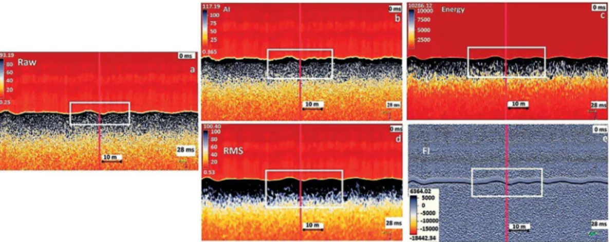
Figure 6. Example of seismic line with/without seismic attribute. In a, a raw record; b, with Instantaneous Amplitude attribute (AI);
c, with Energy attribute; d, RMS Amplitude attribute; e, Instantaneous Frequency attribute.
Comparing
different
seafloors
compositions
Figure 7 indicates the comparison of diferent sealoors, characterized by the presence of rock, shallow-gas and unconsolidated sediments using Seismic Attributes, AI, RMS, Energy and FI, respectively. Note in the Amplitude Attribute that gas and rock have higher values, probably because rock and shallow gas are both characterized by strong relection of the signal, resulting in high amplitude.
For the Instantaneous Amplitude attribute (Figure 7A) it may be noted that the rocky and gassy seafloors have much higher values (about 4,000-20,000 times higher) relative to unconsolidated sediments (with a range of values assigned to rock slightly lower than that
obtained for the gas range feature). This is explained by the fact that rock has a characteristic strong reflection signal, resulting in high amplitude.
The Kruskal-Wallis analysis distinguishing between sediment, rock and gas using the RMS Amplitude attribute is shown in igure 7B. This attribute also efectively diferentiated unconsolidated sediment from rock and gas, the gas feature having the highest amplitude values (between 11,000 and 21,000). The rock showed a greater range of amplitude values (between 6,000 and 20,000).
Figure 7. In A: boxplot analysis using rock, unconsolidated sediment and gas for Amplitude Instantaneous attribute; in B: boxplot analysis using
rock, unconsolidated sediment and gas for Amplitude RMS; in C: boxplot analysis using rock, unconsolidated sediment and gas for Energy attribute; in C: boxplot analysis using rock, unconsolidated sediment and gas for Instantaneous Frequency attribute.
and 498,000,000). The energy attribute had a higher value range for rock (between 70,000,000 and 300,000,000) than shallow gas.
The Instantaneous Frequency attribute (Figure 7D) was the only one that showed a diferentiation between the features analyzed. Sediments had a higher frequency range (between 0.20 kHz and 10.50 kHz). Rock features presented a frequency band between 2.25 kHz and 6.70 kHz, and gas features presented the lowest range - between 0.70 kHz and 2.10 kHz.
Comparing different grain sediment
classes
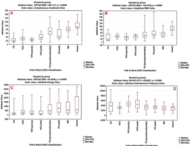
In general, the amplitude attributes enabled us to discriminate between ine and coarse sediments, but no analysis grading the ine class was, or course, apparent.
The Instantaneous Amplitude attribute (Figure 8A) shows the lowest values (ranging between 8 and 160) for ine-grained
sediments. It is possible to note a tendency to increasing attribute value with increasing grain-size; this is also observed in the Spearman correlation coeicient. This parameter is signiicant at 0.62, i.e., a moderate positive relationship between the grain size (mm) and the attribute value.
Another consideration relates to the different attribute values assigned to the fine-sand. This class contains two sub-classes related to the sorting, poorly/ moderate and well sorted. Analyzing these sub-classes in the light of Table 2 it can be said that a large proportion of fine poorly/moderately sorted samples present coarse skewed asymmetry, providing higher attribute values (ranging between 10 and 150).
Figure 8. In A: boxplot analysis distributed in diferent grain classes sub-grouped according to sorting by Instantaneous Amplitude attribute; in
B: boxplot analysis distributed in diferent grain classes sub-grouped according to sorting by Amplitude RMS; in C: boxplot analysis distributed in diferent grain classes grouped according to sorting by Energy attribute; in C: boxplot analysis distributed in diferent grain classes sub-grouped according to sorting by Instantaneous Frequency attribute. CS=Coarse Silt; VCS=Very Coarse Silt; VFS=Very Fine Sand; FS=Fine Sand; MS=Medium Sand; CS=Coarse Sand.
2) the ine sand, including medium sand and coarse sand (SFMC - Sand ine, medium and coarse). However, it is diicult to obtain a more speciic division between the classes.
According to Figure 8B, the RMS Amplitude attribute, ranging in value between 6 and 190, was less eicient in separating grain classes than the Instantaneous Amplitude attribute. In general, the classes of silt, very ine sand, ine sand and medium sand were diferent from that of coarse sand, but showed very little distinction among them. There was a signiicant diference between the silt-very ine sand and the coarse sand classes. Note in the graph that there is an increase in the value of the attribute with increasing grain size, a fact evidenced by the Spearman coeicient, which was signiicant and moderate with a value of 0.41.
This lower value of the Spearman coeicient (compared to the Instantaneous Amplitude) can be explained as due to
the fact that the greatest attribute values are not assigned to the coarse sand class but rather to the ine sand class. As the asymmetry of the ine sand class is variable, and it is not possible to establish a trend in asymmetry whether towards coarse sediment or ine since the samples are from diferent locations, it can be said that the attribute value may be associated with the other characteristics of the sediment, for example composition and morphological properties.
high values assigned to all grain classes even in the iner grade ones such as silt and very ine sand.
In Figure 8D it may be noted that the Instantaneous Frequency attribute was not as efective as the amplitude attributes in discriminating between diferent grain classes. The Instantaneous Frequency displayed two distinct behaviors, the silt and very ine sand classes have a tendency to show increased attribute value, while the ine, medium and coarse sand classes have the opposite behavior. As a consequence, this attribute presented the low Spearman coeicient of 0.10.
DISCUSSION
As regards sorting, asymmetry and kurtosis, correlation between the irst parameter and seismic attributes presented the best result. Sorting was investigated because it is an important parameter for describing the samples of more heterogeneous composition which may present diferent packaging arrangements, which inluence the density, porosity and permeability of the material (JACKSON, 2007).
Comparing
different
seafloors
compositions
Figure 5 shows the 3 eco-characters observed in seismic proiles, including unconsolidated sediment, gas and rock. Considering the seismic records indicating sand, though these sediments usually have a higher density and thus greater impedance, this sediment has higher relection amplitude as compared to the echo character of smaller sediment grain size (JACKSON, 2007). As described above, rock and gas eco-characters have speciic characteristics, which can be easily identiied in seismic proiles. Shallow gas was usually identiied by multiple seismic attributes and causes the masking of adjacent relectors. In the analyzed proiles the gas was a shallow feature, found at the interface between sealoor and water, and is formed from the decomposition of organic matter.
When analyzed in comparison with unconsolidated sediment, gas and rock show higher amplitudes when amplitude attributes are analyzed. This is because shallow gas is associated with ine-grained sediments (FRAZÃO; VITAL, 2007), and when the gas is close to the water/seabed interface it forms a strong impedance contrast, because the speed of the acoustic wave decreases considerably when it comes into contact with the gas
(WILKENS; RICHARDSON, 1998), thus constituting a boundary that will relect a great amount of energy.
It was not possible to determine which feature had higher amplitude attribute value, because each one presented a diferent behavior for each attribute. IA and RMS showed higher values for gas, while Energy indicated the highest values for rock. These diferences may occur during the tracing of the horizon because in OpendTect the horizon is created manually, i.e., there might be uncertainties regarding the position of the amplitude peak.
The Instantaneous Frequency was the only attribute able to diferentiate between rock, gas and unconsolidated sediment. The larger variability of this attribute observed in sedimented sealoors can be explained by diferences in the compositions, characteristics and morphometric parameters of the particle size curve for selected samples.
Comparing different grain sediment
classes
No relationship between seismic attributes and the sorting of unconsolidated sediments was observed. When comparing well-sorted very ine sand and ine sand we did not observe any real distinction between them, indicating that sorting is not the main property that determines attribute value. In the literature, no such comparison is found. The most common use made of Instantaneous Amplitude is to emphasize the continuity of relectors, to highlight the presence of channels, or to enhance deeper relectors.
The RMS amplitude attribute gave a signiicant and moderate Spearman coeicient (0.41). This intensity can be explained as resulting from the fact that the highest attribute values were not assigned to the coarse sand class but to ine sand. Coarse sand is poorly sorted and symmetrical, while ine sand has varied sorting and symmetry; in this case, variability could be explained by changes in other sediment characteristics and properties such as, for example, composition and morphological properties.
Figure 9. On the left may be seen the attribute values for Balneário Camboriu city, in B is the zoom of area A; the right side showing the attribute
value for Aracaju city (C). Source: Google Earth.
assigned to all classes of grains even to the smaller-sized classes such as silt and very ine sand.
The Instantaneous Frequency attribute presented two distinct kinds of behavior. The silt and very fine sand classes have a tendency to increase attribute value (the value ranging between 0.4 kHz and 10.5 kHz), while fine, medium and coarse sand classes have the opposite trend (a value range of between 0.2 kHz and 6.6 kHz), resulting in a low positive Spearman’s correlation (0.10). This might also be explained by the different frequency bands (and the different equipment used) of seismic sources and by the uncertainties involved in tracing the horizons.
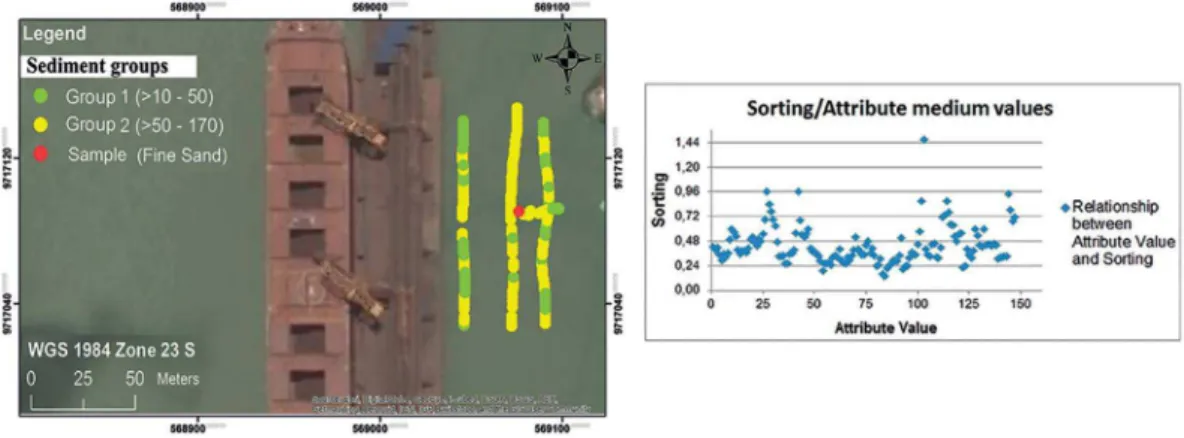
Model Validation
Before the analysis, two seismic proiles containing the samples collected were separated to validate the results. The attribute with the highest eiciency in discriminating between diferent sealoors, the Instantaneous Amplitude, was calculated for these two lines and the results analyzed. Considering the two groups proposed: SVFS (the silt and very ine sand group) and SFMC (the ine, medium and coarse sand group), the limits for the attribute values were deined: between 10-50 for the SVFS group; and between 50-175 for
the SFMC group, taking as a reference the minimum value and variability range of between 25 and 75%.
Analyzing Figure 9A and Figure 9B, it may be seen that there are a large number of samples of the SFMC group characterized by a coarser grain size, and this may be conirmed by the number of samples located on the same proile. In Figure 9C the SVFS group was predominant and the silt and very ine sand classes can be conirmed by the number of samples collected on the same seismic line.
After the test with two seismic lines, the method was applied to a small area (containing a collected sample) in Ponta da Madeira Port Terminal in São Luís (Figure). Ponta da Madeira Port Terminal is part of the Maranhão Port, located in São Marcos Bay, on the west coast of São Luís Island.
Figure 10. On the left: sample and attribute value distributions, where Group 1: SVFS and Group 2: SFMC. On the right: the ratio of
the average Instantaneous Amplitude attribute values and sorting. Source: Google Earth.
attribute values and sorting. The range (minimum and maximum) of ine sand sample sorting, between 0.12 and 0.63, indicates that values above that range are composed of particles larger than ine sand and that below this range they would be even smaller than ine sand.
In this paper we tested the ability of Seismic Attributes to discriminate between diferent sealoors. Concerning the sealoors covered by unconsolidated sediments, we used Seismic Attributes to discriminate between diferent grain sizes, and were able to provide a division into two groups: the silt and very ine sand (SVFS) group and the ine, medium and coarse sand (SFMC) group. On the other hand, these attributes were not eicient in providing a iner discrimination. For this purpose, the Instantaneous Amplitude was more eicient in distinguishing between the two groups relative to the Energy attribute. The Instantaneous Frequency attribute showed a diferent behavior: in the SVFS group there was an increase in the frequency range, while in the SFMC group there was a decrease in the frequency range.
Comparing diferent sealoor types, i.e., those characterized by the presence of shallow gas and rock, the amplitude attributes were efective in distinguishing the sediments from shallow gas/rock, but did not diferentiate between shallow gas and rock. The two features had very high, though similar, amplitudes. On the other hand the Instantaneous Frequency attribute was efective in diferentiating between sediment, rock and gas, with sediment presenting a higher band, rock an intermediate band and gas the lowest one.
For a better development of the subject in future studies, it is suggested that other kinds of information should be considered to describe the behavior of the seismic waves - such as the material composition (the amount of carbonate, organic matter), parameters of the grading curve, structural and morphometric characteristics (angularity, tortuosity, rounding, arrangement, packing), porosity and density. In addition the conditions under which the survey was undertaken should also be considered.
These would include the sea conditions: a ripple can modify the stability of the equipment and thereby alter the angle of the beam striking the background from various angles, depending on whether the equipment has been attached to the vessel or is being towed. Even when the same equipment is used, diferent frequency bands can be selected, and thus modify the attributes that correspond to a particular frequency. Further, the equipment’s power supply used during data acquisition directly inluences the amplitude values obtained. The parameters such as sea water temperature, salinity and suspended material, for example, are responsible for attenuating the acoustic signal by changing the response of the attributes.
ACKNOWLEDGMENTS
REFERENCES
AYRES NETO, A. Uso da sísmica de relexão de alta resolução e da sonograia na exploração mineral submarina. Rev. Bras. Geof., v. 18, n. 3, p. 241-256, 2000.
BLOTT, S. J.; PYE, K. GRADISTAT: a grain size distribution and statistics package for the analysis of unconsolidated sedi-ments. Earth Surf. Process. Landf., v. 26, n. 11, p. 1237-1248,
2001.
CHOPRA, S.; MARFURT, K. J. Seismic attributes - A historical perspective. Geophysics, v. 70, n. 5, p. 3SO-28SO, 2005.
CHEN, Q.; SIDNEY, S. Seismic attribute technology for reser-voir forecasting and monitoring. Lead. Edge, v. 16, n. 5, p.
445-456, 1997.
DAMUTH, J. E. Echo character of the western equatorial Atlantic loor and its relationship to the dispersal and distribution of terrigenous sediments. Mar. Geol., v. 18, n. 2, p. 17-45, 1975.
DAMUTH, J. E. Echo character of the Norwegian-Greenland Sea: Relationship to Quaternary sedimentation. Mar. Geol., v.
28, n. 1-2, p. 1-36, 1978.
DIAS, J. A. A análise sedimentar e o conhecimento dos sistemas marinhos. Faro: Universidade Federal de Algarve, 2004. 80 p.
FALCÃO, L. C.; AYRES NETO, A. Parâmetros físicos de sedi-mentos marinhos supericiais da região costeira de Caravelas, sul da Bahia. Rev. Bras. Geof., v. 28, n. 2, p. 279-289, 2010.
FOLK, R. L.; WARD, W. C. Brazos River bar: A study in the signiicance of grain size parameters. J. Sediment. Petrol., v.
27, p. 3-26, 1957.
FRAZÃO, E; VITAL, H. Estruturas rasas de gás em sedimentos no estuário Potengi: Nordeste do Brasil. Rev. Bras. Geof., v.
25, suppl.1, p. 17-26, 2007.
JACKSON, D. R.; RICHARDSON, M. D. High-Frequency
Sea-loor Acoustics. New York: Springer, 2007. 573 p.
JONES, E. J. W. Marine Geophysics. Chichester: Wiley, 1999.
466 p.
LANDMARK. PostStack Family Reference Manual. Houston:
Landmark Graphics Corporation, 2004. 138 p.
MCGEE, T. M. High-resolution marine relection proiling for engi-neering and environmental purposes. Part A: Acquiring analogue seismic signals. J. Appl. Geophy., v. 33, n. 4, p. 271-285, 1995.
ROSA, A. L. R. Análise do Sinal Sísmico. Rio de Janeiro:
Socie-dade Brasileira de Geofísica, 2010. 668 p.
SHAPIRO, S. S.; WILK, M. B. An Analysis of Variance Test for Normality (Complete Samples). Biometrika, v. 52, n. 3-4, p.
591-611, 1965.
SIEGEL, S. Nonparametric statistics for the behavioral sciences.
New York: McGraw-Hill, 1956. 307 p.
TANER, M. T.; KOEHLER, F.; SHERIFF, R. E. Complex seismic trace analysis. Geophysics, v. 44, n. 6, p. 1041-1063, 1979.
TANER, M. T. Seismic attributes. Recorder, v. 26, n. 7, 14 p.,
2001.
WILKENS, R. H.; RICHARDSON, M. D. The inluence of gas bubbles on sediment acoustic properties: in situ, laboratory,
and theoretical results from Eckernförde Bay, Baltic sea.