A
r
ti
c
le
Printed in Brazil - ©2008 Sociedade Brasileira de Química 0103 - 5053 $6.00+0.00
*e-mail: [email protected]
Determination of Liquefied Petroleum Flame Temperatures using Emission Spectroscopy
Dermeval Carinhana Jr.,*
,aLuiz G. Barreta,
aCláudio J. Rocha,
aAlberto M. dos Santos
aand Celso A. Bertran
baInstituto de Estudos Avançados, CP 6044, 12228-970, São José dos Campos-SP, Brazil
bInstituto de Química, Universidade Estadual de Campinas, CP 6154, 13084-862 Campinas-SP, Brazil
A espectroscopia de emissão foi utilizada na determinação da temperatura de chamas pré-misturadas de GLP. Investigou-se a emissão natural de radicais CH* em três diferentes condições
de queima: razão estequiométrica de combustível/oxidante, excesso de combustível (chama rica) e excesso de oxidante (chama pobre). O valor médio obtido para a temperatura rotacional de CH* foi de 2845o70 K nas condições utilizadas nos experimentos. Esse valor não variou
significativamente com os demais tipos de chama e é compatível com os cálculos de temperatura adiabática dos sistemas estudados. Essa temperatura também é concordante com resultados obtidos por via indireta, utilizando-se o método de linha reversa de sódio, que consiste em uma técnica bem estabelecida e independente da emissão natural. Temperaturas vibracionais de ca. 4600 K foram calculadas, indicando que o tempo de vida do CH* não é suficiente para que o equilíbrio
entre os modos rotacionais e vibracionais seja estabelecido.
Emission spectroscopy was used in the temperature determination of LPG (liquefied petroleum gas) premixed flames. Natural emission of CH*radicals was investigated in flames under three
different burning conditions: fuel/oxydizer stoichiometric ratio, fuel excess (rich flame), and oxidizer excess (lean flame). An average value of 2845o70 K was obtained for CH*rotational
temperature in the set up used in the experiments. This value did not show significant change with the type of flame analyzed and it is compatible with the calculated adiabatic flame temperatures of the investigated systems. This temperature value also agrees with that determined by an indirect measurement, using the sodium line reversal method, which is independent from the radical natural emission and well established in literature. Vibrational temperatures of ca. 4600 K were calculated, indicating that the CH* lifetime is insufficient for the establishment of an equilibrium
state between the rotational and vibrational modes.
Keywords: chemiluminescence, premixed flames, Boltzmann distribution, combustion diagnostics
Introduction
In an adiabatic flame all released heat by exothermic chemical reactions, at constant pressure, is absorbed by the combustion products, without heat transfer to the surroundings.1 This temperature corresponds to the highest
temperature that can be achieved by a flame. However, the lack of thermal equilibrium in a real flame does not permit the use of the classical temperature concept, as a kinetic energy measurement, in these systems. Nevertheless, in this case we may consider the concepts of rotational temperature, vibrational temperature and electronic
temperature.2-6 In flames, rotational temperature is very
close to the kinetic temperature, due to the quick transfer between translational and rotational energies.7 In this way,
rotational temperature measurement is as a good indicative of flame temperature.
Flame temperature determination provides important information about released heat resulting from chemical reactions in combustion systems.8 Temperature distribution
knowledge in a combustion chamber may indicate eventual project problems and the necessity of construction optimization of these devices.9 Temperature diagnosis,
characteristics. The values obtained correspond to an average measurement, especially in the case of small flames.8 In thermocouple applications, a large radical
concentration in flames may induce catalytic processes on its surface, resulting in significant errors in temperature determination.9
Contrary to the aforementioned latter methods, radiation emission and absorption, on the other hand, by hot gas flames have an absolutely non-intrusive characteristic. Both, especially emission, offer the possibility of temperature monitoring and excited state studies from the ultraviolet to infrared spectra.10,11 Most of the optical methods are based
on lasers, as laser absorption spectroscopy, laser induced fluorescence (LIF), Raman spectroscopy and coherent anti-Stokes Raman spectroscopy (CARS).12 However, these
techniques can not be applied in some situations, due its complex experimental apparatus.13 In fact, the real time
monitoring of temperature of some airborne combustion systems, such as aircraft turbines or rocket engines, is very complicated, or impossible, when employing laser devices which require less drastic working conditions. Mechanical vibrations, for example, can easily damage the system alignment. In this case, natural emission of species presents in flames has been used.14-16 Besides
non-intrusive characteristic and simpler requirements, emission spectroscopy is also favored by the nature of the probe species. First, flame emission is strongly associated to the diatomic molecules. Spectroscopy constants for these species are very well determined, which required lower calculations for temperature determination. Second, natural emission occurs near the region where they were generated, due to their small emission life time.17 This
can be used to relate the information obtained from flame emission spectra to the temperature or concentrations at a specific flame region.5
Spontaneous or natural emission in flames is due to chemical reactions that produce chemical species in excited state. This phenomenon is also known as chemiluminescence. The most intense emissions are due to C2*, CH* e OH* species.18,19 OH* has been the most used
radical in flame temperature determination, since this species can be found in substantial concentrations in the hot zones of most flames.9 However, measured temperatures
in an atmospheric methane flames using natural emission technique showed values hundreds of degrees higher than flame adiabatic temperature.20,21This abnormal behavior
was associated to the a non-equilibrium state of OH* in
the flame inner cone.
Radical CH*has been used in flame mapping, due to
its also intense emission bands in the ultraviolet-visible spectrum,22 which is concentrated mainly in the flame
inner cone. CH* radical most intense emission band system
is observed around 431.5 nm, which corresponds to the (A2$-X20) transition.23 The Q branch of 0-0 vibrational
band originates a strong peak at 431.25 nm. In this spectrum region, there is also the presence of 1-1 vibrational band, less intense. At 432.4 nm an intense peak is observed attributed to the 2-2 vibrational band.
CH* natural emission was used to determine temperatures
in the past. Most studies have focused on low pressure plasmas and flames,14,15,24,25 which allow better conditions
to understand the combustion processes investigated. In this situation, lower collision ratio, if compared to atmospheric flames, produces a more specific radical deactivation process, which returns a less complex emission spectrum. This allows faster and simpler calculations of rotational or vibrational temperatures and, additionally, of some spectroscopy parameters, such as rotational and vibrational energy transfer ratios.26 However, in
low pressure conditions, the frequency of collisions for diatomic radicals is sufficient to establish the equilibrium of the rotational states, i.e., a Boltzmann’s distribution, but may not be enough for thermal equilibrium. Thus, in these cases, we cannot take rotational temperature as flame temperature. Atmospheric systems also were studied by natural emission, but to a lower extent. Additionally, results are inconclusive: measurements in atmospheric acetylene flames returned an over-adiabatic rotational temperature,18
while other studies with atmospheric plasmas showed that CH*rotational temperature can be assigned to the gas
temperature.27
The aim of the present work is to establish a reliable non-intrusive method of temperature determination of the atmospheric combustion system by emission spectroscopy. The development of this method is part of a Brazilian effort to project and construct hypersonic vehicles, commonly named “scramjets”. In these vehicles, combustion takes place at supersonic speeds, generated by hypersonic shock waves, which eliminate the employment of intrusive temperature sensors, such as thermocouples. In this work, Liquefied Petroleum Gas was used as fuel due to its low cost and because at the moment only small organic molecules, mainly methane and acetylene, were studied using optical combustion diagnostic techniques.
Temperature calculation
between the peak intensity (I) and the temperature (T) is given by (1):15,28
(1)
where SJ´J” is the line strength of a transition from the upper (J´) and lower (J”) rotational state; EJ´ is energy of the upper level and C a proportionality constant. In a good approximation, if we consider a group of emission lines of the same ro-vibronic band, the vibrational and electronic part of the line strength are equal for all transitions in the band. So, if the system presents a Boltzmann distribution, a plot of natural logarithm of line intensities versus energy level returns a straight line, whose slope is the inverse of rotational temperature.
As mentioned in Introduction, temperature calculation in atmospheric flames by using natural emission technique has shown some results that are not reliable. Thus, in this study we employed another technique to validate natural emission temperature results. The chosen technique was line reversal method.29,30 This method is based on the
measurement of electronic temperature of ions inserted in flames. The most common is the Na+ species. Although it
is an intrusive process, this is a simple and well established method, which has been largely used in the last decades. This method is based on Kirchhoff’s law, which states that for a gas in thermodynamic equilibrium the emissivity (A) is equal to the absorption coefficient (E) values. Temperature is determined by comparison between the emission intensity of a seeded species in the flame, usually sodium atoms, and the radiation from a black body, simulated by a heated lamp filament, transmitted through the flame hot gases. In this situation, the total radiation flux (&) which reaches the light detector is given by:
& = &f + (1 – E)&lamp (2)
where&fl is the radiation flux emitted by the flame, (1-E) is the flame transmittance and &lamp is the flux emitted by the filament lamp. All & values depend on the solid angle (7) of the employed optics, the radiation wavelength (L) and the emitters temperature (T).
In an experimental apparatus where 7 is kept constant and the used spectral range is sufficiently narrow, & is an exclusive function of T. If the validity of Kirchhoff´s law is assumed, i.e.,E = A, the system shows no difference between absorbed and emitted radiation by the flame. This condition makes the comparison between &fland
&lamp possible. Consequently, the relation between &
and T is:
a)&f > &lamp Tf > Tlamp
b)&f = &lamp Tf = Tlamp (3)
c)&f < &lamp Tf < Tlamp
where Tfl and Tlamp are the flame and the lamp temperatures respectively. Equation 3b, shows the so-called inversion point,i.e., where both flame and lamp spectra show the same intensity and, as consequence, the same temperature. If the lamp temperature is calibrated against another temperature standard, such as optical pyrometers, flame temperature can be determined.
Despite the relative instrumental simplicity and reliability of the line reversal technique, there are some conditions which may affect the temperature results, such as solid particles in flames or the presence of a cool boundary layer.29 Solid particles, like soot, seed, ash or unburned fuel,
act as black body emitters and absorbers, and also scattered radiation out of the lamp incident beam. This superimposed effect makes the determination of the real reversal point difficult. The presence of a cool boundary layer produced by a broadening of atomic emission line causes a re-absorption of the radiation emitted by the center of the line, which diminishes the temperature obtained. However, effects can be neglected in several cases. Flames with equivalent ratio fuel/oxidant near 1.0 (stoichiometric condition) do not present unburned fuel and do not produce soot or ash. In the same way, small open flames, like atmospheric flames, do not show remarkable differences of temperature between bulk and boundary layer regions. Thus, this technique can be used to validate natural emission results without any corrections.
Experimental
Ro-vibrational emission spectra of CH* radicals were
used to determine the temperature of liquefied petroleum gas (LPG) flames, for three different equivalence ratios:
F = 0.78 (lean flame), F= 1.02 (stoichiometric flame) andF = 1.43 (rich flame). A premixed type home-built burner based on a previous published work was used in the experiments.31 State-steady flames were produced from a
gaseous mixture of LPG/atmospheric air/oxygen. The extra oxygen was used to achieve the desired equivalence ratio. Several gas flows were tested and the three combinations which produced more stable flames were selected. These correspond to the effective work range of the burner used,
The optical system used consisted of a TRIAX 550 (Jobin Yvon) monochromator of 0.5 m focal length (f), equipped with a 1200 lines mm-1 diffraction grating,
with blaze at 500 nm. The slit width was fixed at 10Mm. Emission signal was detected by a Hamamatsu R928P phototube, with 950 V as work voltage. Spectra were obtained at 415 to 440 nm range, which correspond to A2$l X30 electronic band of the CH* radical. With these
experimental conditions, the spectral resolution obtained was ca. 0.04 nm. This value was determined by a calibration with a Hg discharge lamp.
The burner was mounted on a translation stage with mobility in the three orthogonal directions (x, y and z). This set up allowed spectra recording at different distances above burner along the principal flame axis, at regular intervals of 1 mm, starting at the initial value of 2.5 mm (with reference to the outlet of the burner) and ending at the maximum value of 22.5 mm.
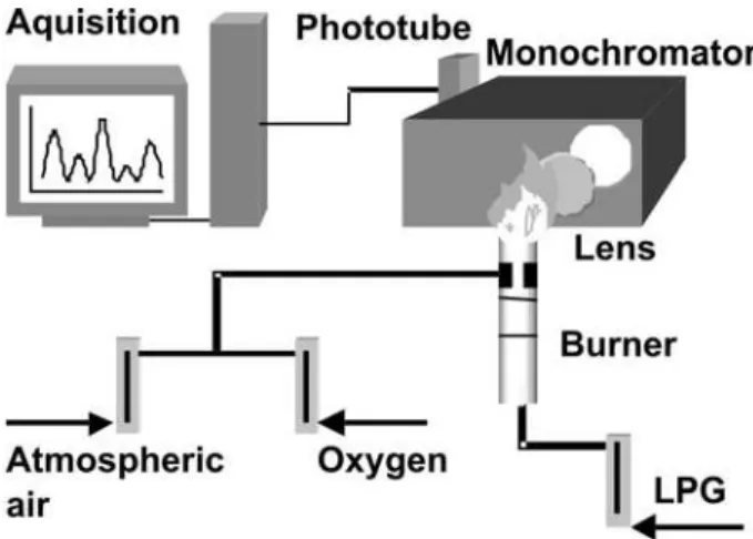
A quartz lens, with f = 100 mm and diameter of 2” was used for light collection. The flame image was projected on the spectrometer entrance slit in a 1:1 ratio. All intensities were corrected by optical response curves of the employed gratings and phototube given by the manufacturers. The apparatus scheme is shown in Figure 1.
Rotational temperature was determined by comparison between experimental and simulated spectra. These were calculated using a free code, named LIFBASE.32 This
software has an internal data bank containing all useful molecular spectroscopy data for many diatomic species important in combustion, including the CH*radical. With
LIFBASE, spectra were simulated at different temperatures and compared, in an interactive graphic interface, with experimental data. Temperature values were assigned according to the better agreement between both spectra, using as reference the statistical parameter variance, i.e., the sum of the square of the intensity deviations. The overall experimental spectral resolution was also required. This parameter is generally defined as the full-width at the half-height peak. Flame adiabatic temperatures were calculated by the free software GASEQ.33
Radical temperature was also determined using the Boltzmann plot method, described in Introduction. We used the full peak intensity at the half-width for rotational temperature calculations. Spectroscopic data employed in this method were obtained in literature works.15,34 For
the sodium line reversal experiments, Na was seeded in the flame, inserted as NaCl crystals. A lamp (100 W) was employed as the irradiation source. Lamp temperature calibration was carried out with a tungsten filament optical pyrometer (Keller Pb06/01 AF3) up to 3300 K. The set up shown in Figure 2 was used from several experimental arrangements mentioned in the literature due to its simplicity.30
Results and Discussion
No remarkable differences were observed in the emission spectra of the flames studied in this work. A spectrum of CH* for a stoichiometric flame measured at
2.5 mm above the burner is shown in Figure 3.
The CH* emission has an intensity maximum at
431.5 nm. In this region, there is an overlapping of its 0-0
Table 1. Burner conditions used in chemiluminescence measurements Flame / (F) Total O2/
(mmol min-1)
N2/ (mmol min-1)
LPG / (mmol min-1)
Rich (1.43) 21.2 27.9 6.3
Stoichiometric (1.02) 35.5 27.9 6.3
Lean (0.78) 46.8 27.9 6.3
Figure 1. Experimental apparatus utilized in spectra records.
Figure 2. Experimental apparatus utilized in line reversal
and 1-1 vibrational bands, as well as an isolated peak at 432.4 nm which corresponds to the 2-2 band. The spectral range between 416 and 425 nm is formed predominantly by the R-branch 0-0 band, with J values from 11 to 20. For
Jq7 this branch shows a rotational structure well spaced with no interference from other peaks (Figure 4).35 This
region, which appears as doublet peaks, was used for the rotational temperature determination.
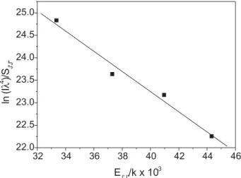
Rotational temperatures were determined from the slope of the straight lines obtained according to Equation 1. The longer wavelength peaks of the doublet were used in the experimental measurements of the peak intensities. SJ´J and EJ´ were taken from the literature.15 Figure 5 corresponds
to a typical Boltzmann’s plot obtained from an average of three experimental spectra of a stoichiometric flame, at 2.5 mm above the burner. Each point in the graphic, therefore, corresponds to the average measured intensity, the straight line was calculated by linear regression and
the rotational temperature determined from the slope of the line. Error temperature corresponds to the standard deviations of the temperature calculations.
Plot linearity indicates that radical CH* population of the
rotational energy states presents a Boltzmann´s distribution. Similar plots were drawn for other experimental conditions and the results are summarized in Table 2 and Figure 6. The shown errors correspond to the standard deviation of the whole spectral data at each distance above the burner.
According to Figure 6, the emission signal could be observed only up to a distance of 3.5 mm for stoichiometric and 5.5 mm for rich flames. For higher distances, the intensity signal decreased sharply and could not be detected. Rotational temperature values did not show an appreciable variation with the equivalence ratio within the range of distances above the burner studied. The rich-flame temperature at 4.5 mm returned an over-adiabatic temperature value, probably due to an error in the flow meter set, i.e., the temperature determined corresponds to another flame composition. However, in general the
Figure 3.CH* ro-vibrational spectra. Stoichiometric flame. Distance from burner of 2.5 mm.
Figure 4. Experimental spectrum corresponding to R-branch 0-0 CH* vibrational band.
Figure 5. Average Boltzmann’s plot for CH* spectra. Stoichiometric flame. Distance from burner of 2.5 mm. Calculated rotational temperature = 2830o 47 K.
Table 2. Experimental temperatures for CH* radical as a function of equivalence ratio (F) and burner distance (mm)
Distance / mm T / K
F= 1.43 F= 1.02 F = 0.78
5.5 2793o71 ---
---4.5 2965o66 ---
---3.5 2878o125 2783o26 2872o76
2.5 2784o60 2859o47 2817o58
temperature distribution suggests an adiabatic behavior in the investigated flame region, corresponding to the inner cone of the flame, which is the mostly responsible for the chemiluminescent process in the flame. Indeed, rotational temperature values are very close to the flame adiabatic temperature: 2857 K, 2946 K and 2910 K for rich, stoichiometric and lean flames, respectively. If one assumed an adiabatic behavior of the analyzed region, the average value for CH* rotational temperature of the butane
flames investigated in this work is 2845o70 K. Again, the measurement errors were calculated from the standard deviation of the whole set of temperature values.
In LIFBASE simulations, we chose the same spectral range as in the Boltzmann’s plots (R-Branch region). An example of the comparison between experimental and simulated spectra is shown in Figure 7. The determined experimental spectral resolution was ca. 0.45 nm.
There is a good agreement between both spectra shown in Figure 7. Besides R-branch region, rotational temperatures were also determined from the A-X transition band head (Figure 8). Spectra agreements are very good in the all wavelength region, with exception of the peak between 432 nm and 433 nm. As mentioned before, this peak corresponds to the 2-2 vibrational band envelope.
A detailed spectra analysis shows that theoretical peak intensity is much lower than the experimental one. This indicates a larger number of excited species in vibrational level U’ = 2 than expected in a thermal equilibrium system. This condition was observed in all the simulations. As discussed in Introduction, temperature concept only can be adopted in a system in thermodynamic equilibrium. In this case, temperature can describe several system properties, among them: all particle velocity distributions are in agreement with Maxwell’s equation; excited state populations agree with Boltzmann’s equation; and the electromagnetic radiation distribution corresponds to Planck’s law.6,36 Other processes are related to detailed
knowledge of all chemical reactions, ionizations and dissociations which occur in the system. In flames, these conditions are not quite achieved. In the inner cone reaction zone, for example, species do not have sufficient time for establishing equipartition of released chemical energy by chemiluminescent processes among the system freedom degrees. As the species leave the reaction zone, translational and rotational energies achieve equilibrium rapidly. However, vibrational and electronic levels relax more slowly. Former considerations permit a better understanding about 2-2 vibrational band. CH*
is not formed by thermal excitation, in most reaction mechanisms presented in literature.37 Thus, chemical
Figure 6. Experimental temperatures for CH* radical as a function of equivalence ratio (F) and distance above burner (mm).
Figure 7. Comparison between simulated and experimental CH* spectra. Stoichiometric flame. Zoom at R-Branch region. Distance of 2.5 mm. T = 2912 K for simulated spectrum.
Figure 8. Comparison between simulated and experimental CH*
species in rotational and vibrational excited energy levels would be subjected to collisional deactivation due to the chemical environment. From the obtained temperature, we can say that there is a Boltzmann equilibrium between rotational and translational energies for the investigated flame conditions. However, the intensity difference between the theoretical and experimental 2-2 band suggests that the vibrational modes still do not achieve the equilibrium with the rotational modes of 0-0 vibrational band. In fact, a study of low-pressure methane plasma showed that the 2-2 band lifetime is significantly lower than 0-0 band: 32 ns and 45 ns, respectively.38 To confirm this observation CH*
vibrational temperature was determined.
The major problem in CH* vibrational temperature
determination is the band overlapping that occurs in the studied spectral range. Nevertheless, this problem was resolved in the LIFBASE simulations, as the vibrational bands can be treated separately. The vibrational bands available in LIFBASE are: 0-0, 1-1, 2-2 and 3-3. The integrated area of the former vibrational bands was used for temperature determination by Boltzmann’s method. Figure 9 shows an example of this determination. All the results obtained are listed in Table 3.
According to Table 3, vibrational temperatures are significantly higher than rotational ones. As can be observed, there is no significant difference between the temperatures of each investigated flame neither in the distance above burner. This also contributed to the adiabatic behavior interpretation assigned to the flame region studied. Therefore, the calculated average vibrational temperature for the butane flames is 4600o 127 K. The measurement error is the standard deviation of all temperature listed in the Table 3. Although vibrational temperatures are higher, compared to the rotational ones, these results are in agreement with the concept of both temperatures. Studies have appointed which rotational and vibrational relaxation rates for diatomic hydrides are dependent on the chemical environment. Nevertheless, for CH* radical
the vibrational deactivation is very slow.39 Studies of the
CHBr3 photolysis showed that vibrational energy transfer is more than an order of magnitude slower than rotational energy transfer.24 Thus, vibrational modes need thousands
of collisions, while translational and rotational modes attain equilibrium with few collisions.6 Therefore, CH*
spontaneous emission, in the investigated flames, occurs before the equilibrium state between the rotational and vibrational modes are achieved.
The non-equilibrium of vibrational and rotational temperatures was reported in other works in literature. Emission spectroscopy of a methane-atmospheric air flame indicated rotational and vibrational temperatures of 1400 K and 4200 K, respectively.3 These distinct values are
attributed to the differences in energy transfer mechanisms for each degree of freedom. Characteristic times of rotational energy transfer and collision are ca. 10-14s and
10-15s, respectively. Thus, colisional processes contributed
to an effective way for rotational relaxation before the CH*
radical spontaneous emission, that CH* radiative half-live
time is ca. 0.56Ms. In this same work, CH* ground state
rotational temperature was determined by CARS, and a value of ca. 1500 K was obtained.
Studies of similar flames used in the present work also determined OH ground state rotational temperatures by LIF.40 The average temperature was ca. 2600 K, very close,
hence, to CH* rotational temperature found by emission
spectroscopy.
Both results, demonstrated that radical at ground and excited states present similar temperatures. This indicates that, although chemiluminescence processes are originated from excited species, CH* radiative half-live time is
long enough to allow a minimum number of collisions to establish equilibrium of the rotational distribution in the excited state and also with the ground state, before spontaneous emission takes place.
Figure 9. Vibrational Boltzmann plot. Distance of 2.5 mm. Lean Flame. Vibrational temperature = 4459 K.
Table 3. CH* Vibrational temperature values
Distance / mm T / K
F= 1.43 F= 1.02 F = 0.78
5.5 4300o109 ---
---4.5 4600o102 ---
---3.5 4650o202 4400o41 4400o116
2.5 4400o95 4650o76 4650o96
Table 4. Temperatures obtained by Na line reversal method as function of equivalence ratio and distance above burner
Distance / mm T / K
F= 1.43 F= 1.02 F = 0.78
4 2805o84 2970o89 2885o87
5 2845o85 3040o91 2945o88
6 2845o85 2945o88 2945o88
7 2845o85 3005o90 3005o90
8 2845o85 3040o91 3005o90
Figure 10. Sodium line reversal. Reversion can be observed at 10.5 V. Stoichiometric flame. Distance of 4 mm. T = 2950 K.
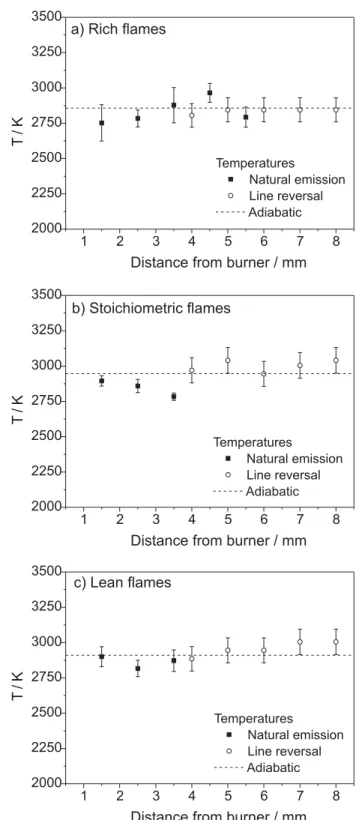
Figure 11. Comparison between line reversal results, CH* rotational temperatures and flame adiabatic temperatures in (a) rich flames, (b) stoichiometrc flames and (c) lean fame.
Emission spectroscopy results support the initial assumption that CH* rotational temperatures can be
considered as a flame temperature indicator. To confirm this hypothesis, flame temperature was determined by another diagnostic method: the sodium line reversal spectroscopy. This technique is totally independent of the CH* natural emission and, as described in Introduction,
is based only in sodium atomic spectrum. Under most burner conditions, sodium electronic temperature can be assigned as translational system temperature.30 An example
of line reversal spectra can be seen in Figure 10. The signal reversal (emission to absorption) is observed at 10.5 V lamp voltages, corresponding to a calibrated temperature lamp of 2950 K.
Results in Figure 10 provide a good idea of the precision of the method. Assuming an error equivalent to half the minor range of the calibrated lamp temperatures, the maximum error is ca. o25 K, hence, under 1% of the calculated flame temperature. To this error, however, it is necessary to add the measurement error from the optical pyrometer used in the lamp calibration. This value, based in statistical estimation, is ca. o2%. Therefore, the maximum error is ca. 3%. Line reversal temperature results are shown
in Table 4. A comparison with CH* rotational temperatures
region, i.e., 3.5 mm. As mentioned before, for this flame composition the intensity signal decreases sharply. Thus, the low rotational temperature can be assigned to poor intensity. However, the maximum deviation between line reversal and CH* natural emission in this region is ca. 6%.
Average line reversal temperature was ca. 2930 K. As observed in natural emission, line reversal temperatures did not show remarkable variation as a function of distance from the burner, within the investigated flame region. With respect to the flame composition, rich flames showed temperatures slightly smaller than stoichiometric or lean flames. This result was expected, due to the lack of oxidant presented in the combustion mixture.
Conclusions
CH* emission spectroscopy was shown to be an
adequate technique for flame temperature determination. Rotational temperature values for this radical were ca. 2850 K. Emission results were compared to the line reversal technique, which correspond to an average flame temperature of ca. 2930 K. Therefore, the non-equilibrium condition reported in the past for rotational temperatures can be rejected in this work. However, this is not true for vibrational modes. Emission spectroscopy showed an average vibrational temperature of ca. 4600 K. This over-adiabatic value can be assigned to the lower ratio of energy transfer for vibrational modes than rotational ones.
References
1. Strahle, W.C.; An Introdution to Combustion, 1st ed., Gordon
and Breach: Amsterdam, 1993.
2. Gaydon, A. G.; Wolfhard, H. G.; Flames, 3rd ed., Chapman and
Hall: London, 1970; Broida, H. P.; J. Chem. Phys.1951,19,
1383; Parker, J. G.; Phys. Fluids1959,2, 449; Kane, W. R.;
Broida, H. P.; J. Chem. Phys.1953,21, 347; Cahen, C.; Sassi,
M.;J. Quant. Spectrosc. Radiat. Transfer1993,49, 281.
3. Wange, J.; Wang, X.; Li, H.; Gu, X.; Spectrosc. Lett.1990,23,
515.
4. Hayashida, K.; Shirai, H.; Amagai, K.; Arai, M.; JSME Int. J.
B-Fluid. T.2002,45, 201.
5. Coitout, H.; Faure, G.; Spectrosc. Lett.1996,29, 1201.
6. Broida, H. P.; Shuler, K. E.; J. Chem. Phys. 1957,27, 933.
7. Lapworth, K. C.; J. Phys. E: Sci. Instrum.1974,7, 413.
8. Chigier, N. In Combustion Measurements; Chigier, N., ed.;
Hemisphere Publishing Corporation: New York, 1991, ch. 1.
9. Kohse-Höinghaus, K.; Prog. Energy Combust. Sci.1994,20,
203.
10. Drakes, J. A.; Pritt, D. W.; Howard, R. P.; Hornkohl, J. O.; J.
Quant. Spectrosc. Radiat. Transfer1997,57, 23
11. Gross, L. A.; Griffiths, P. R.; J. Quant. Spectrosc. Radiat.
Transfer1988,39, 463.
12. Shvartsman, N. A.; Russ. J. Phys. Chem.1975, 49, 1321;
Karpetis, A. N.; Gomez, A.; Combust. Flame 2000, 121,
1; Luque, J.; Crosley, R. R.; Appl. Phys. B1996, 63, 91;
Sandrowitz, A. K.; Cooke, J. M.; Glumac, N. C.; Appl.
Spectrosc. 1998,52, 658; Blevins, L. G.; Renfro, M. W.; Lyle,
K. H.; Laurendeau, N. M.; Gore, J. P.; Combust. Flame1999,
118, 684; Luque, J.; Crosley, R. R.; Appl. Phys. B1996,63,
91; Klein-Douwel, R. J. H.; Jeffries, J. B.; Luque, J.; Smith,
G. P.; Crosley, D. R.; Combust. Sci. Technol.2001,167, 291;
Laurendeau, N. M.; Prog. Energy Combust. Sci. 1988,14,
147; Lederman, S.; Prog. Energy Combust. Sci. 1977,3, 1;
Egermann, J.; Seeger, T; Leipertz, A.; Appl. Opt. 2004,43,
5564; Daily. J. W.; Prog. Energy Combust. Sci. 1997,23, 133;
Seeger, T; Leipertz, A.; Appl. Opt. 1996,35, 2665.
13. Zimmer, L.; Tachibana, S.; Tanahashi, M.; Shimura, M.;
Miyauchi, T.; Proc. 6th Symposium on Smart Control of
Turbulence, www.turbulence-control.gr.jp, accessed in August, 2007.
14. Joklik, R. G.; Daily, J. W.; Pitz, W. J.; Proc. Comb. Inst.1986,
21, 895; Higgins, B.; McQuay, M.Q.; Lacas, F.; Candel, S.;
Fuel2001,80, 1583.
15. Kim, J. S.; Cappelli, M. A.; J. Appl. Phys.1998,84, 4595.
16. Higgins, B.; McQuay, M.Q.; Lacas, F.; Candel, S.; Fuel2001,
80, 1583.
17. Bertran, C. A.; Marques, C. S. T.; Benvenutti, L. H.; Combust.
Sci. Technol.1998,139, 1.
18. Durie, R. A.; Proc. Phys. Soc. A 1952,65, 125.
19. Broida, H. P.; J. Chem. Phys.1953,21, 340.
20. Broida, H. P.; J. Chem. Phys.1951,19, 1383.
21. Fissan, H. J.; Combust. Flame1972,19, 11.
22. Durie, R. A.; Proc. Phys. Soc. 1952,A 65, 125; Broida, H. P.;
J. Chem. Phys.1953,21, 340.
23. Gaydon, A. G.; The Spectroscopy of Flames, 1st ed., Chapman
and Hall: London, 1957; Pearse, R.W.B; Gaydon, A. G.; The
Identification of Molecular Spectra, 4th ed., Chapman and Hall:
London, 1976.
24. Cooper, J. L.; Whitehead, J. C.; J. Chem. Soc., Faraday Trans.
1993,89, 1287.
25. Brennen, W.; Carrington T.; J. Chem. Phys. 1967,46, 7; Math,
N. N.; Savadatti, M. I.; J. Quant. Spectrosc. Radiat. Transfer
1985,34, 75.
26. Crichton, H. L.; Murray, C.; McKendrik K. G.; Phys Chem.
Chem. Phys. 2002,4, 5768.
27. Pellerin, S.; Koulidiati, J.; Motret, O.; Musiol, K.; Graaf, M.
de; Pokrzywka, B.; Chapelle, J.; High Temp. Mater. Processes
1997,1, 493.
28. Herzberg, F. R. S. G.; Molecular Spectra and Molecular
Strucuture, 2nd ed., Van Nostrand Reinhold Company: London,
29. Mak, W. H.; UTIA Techanical Note 1963,66, 1; Thomas, D. L.;Combust. Flame1968,12, 541.
30. Loomis, A. G.; Perrot, G. St. J.; Ind. Eng. Chem. 1928,20, 1004;
Yang, D.; Xu, H.; Wang, J.; Zhao, B.; Spectrosc. Lett.2001,34,
109.
31. Lacava, P. T.; PhD Thesis, Instituto Nacional de Pesquisas
Espaciais, INPE, São José dos Campos, Brazil, 1995. 32. Luque, J.; Crosley, D. R.; LIFBASE; Database and spectral
simulation (version 1.5); SRI International Report MP 99-009, USA, 1999.
33. Morley, C.; GASEQ; Chemical Equilibria in Perfect Gases (version 0.76); www.gaseq.co.uk, accessed in August 2007. 34. Pellerin, S.; Musiol, K.; Motret, O.; Pokrzywka, B.; Chapelle,
J.;J. Phys. D: Appl. Phys.1996,29, 2850.
35. Couris, S.; Anastasopoulou, N.; Fotakis, C.; Chem. Phys. Lett.
1994,223, 516.
36. Reif, I.; Fassel, V. A.; Kniseley, R. N.; Spectrochim. Acta1973,
28B, 105.
37. Smith, G. P.; Luque, J.; Park, C.; Jeffries, J. B.; Crosley, D. R.;
Combust. Flame2002,131, 59.
38. Luque, J.; Juchmann; Jeffries, J. B.; Appl. Opt. 1997,15,
3261.
39. Garland, N. L.; Crosley, D. R.; Appl. Opt. 1985,24, 4229.
40. Dos Santos, L. R.; PhD Thesis, Universidade de São Paulo,
Brazil, 2005.
Received: August 27, 2007
Web Release Date: August 11, 2008