I. INTRODUCTION
The emergence of complex patterns is one of the most dis-tinct signatures of nonlinear interactions in natural systems. Since Einstein’s pioneering work on Brownian motion [1], it became clear that much can be accomplished by modeling the interactions of a system with its environment through the ac-tion of random and viscous forces. During most of the twen-tieth century, studies were mainly restricted to investigating the motion of a point particle in nonlinear potentials [2]. With the advent of fast computers, modeling of stochastic evolution added spatial dimensions, allowing for the quantitative study of spatio-temporal complex behavior. Up to about ten years ago, most of the work concentrated in hydrodynamical and soft condensed-matter systems [3]. Recently, developments in high energy physics and cosmology have opened the inter-esting possibility that complex spatio-temporal behavior may also play a role in relativistic field theories, in particular dur-ing the early stages of cosmological evolution [4] and may even be observed in high-energy colliders [5].
Here we will briefly review some of the work done dur-ing the past few years which focused on understanddur-ing the effects of fast quenches on nonlinear scalar field theories. The quenches model both temperature quenches in the context of fast cosmological expansion (in particular at scales close to the GUT scale∼1016GeV) or the cooling of fireballs during high energy collisions such as those currently being investi-gated at RHIC and soon at LHC. The quench may also repre-sent a pressure quench, common in condensed matter physics or, more generally, the appearance of a low-energy effective interaction that modifies the effective potential of the long-wavelength modes of the field or order parameter describing the system’s evolution. We will conclude with an application of these ideas to inflationary cosmology [6].
II. THE MODEL
Consider a (2+1)-dimensional real scalar field (or scalar or-der parameter)φ(x,t)evolving under the influence of a poten-tialV(φ). The continuum Hamiltonian is conserved and the
total energy of a given field configurationφ(x,t)is,
H[φ] =
d2x
1 2(∂tφ)
2+1 2(∇φ)
2+V(φ),
(1)
whereV(φ) =m22φ2−α
3φ3+λ8φ4is the potential energy den-sity. The parameters m, α, and λ are positive definite and temperature independent. It is helpful to introduce the di-mensionless variables φ′=φ√λ/m, x′ =xm, t′ =tm, and α′=α/(m√λ)(We will henceforth drop the primes). Prior to the quench,α=0 and the potential is an anharmonic single well symmetric aboutφ=0. The field is in thermal equi-librium with a temperatureT. At the temperatures consid-ered, the fluctuations of the field are well approximated by a Gaussian distribution, withφ2=aT (a=0.51 and can be computed numerically). As such, within the context of the Hartree approximation [7], the momentum and field modes in k-space can be obtained from a harmonic effective potential, and satisfy|π(¯ k)|2=T and|φ(¯ k)|2= T
k2+m2 H
, respectively. The Hartree massm2H=1+32φ2depends on the magnitude of the fluctuations (and thusT). Within the Hartree approxi-mation we can write the effective potential as
Veff
φave,m2H
=
1−m2H(t) φave+
1 2m
2
H(t)φ2ave− −α
3φ 3 ave+
1 8φ
4
ave. (2)
Hereafter we will refer to a particular system by its initial temperature. All results are ensemble averages over 100 sim-ulations.
Ifα=0, the
Z
2symmetry is explicitly broken. Whenα=1.5≡αc, the potential is a symmetric double-well (SDW), with two degenerate minima. This is the first case we consider.
III. QUENCHING INTO SYMMETRIC DOUBLE WELLS: EMERGENCE OF SPATIO-TEMPORAL ORDER
Atα=αc=1.5, the quench amounts to switching from a single to a double well with the field initially localized at φ=0. In Fig. 1 we indicate this schematically.
FIG. 1: Schematic picture showing change in potentialV(φ)from single-well to symmetric double-well after quench.
area in 2d). The amplitude of these oscillations is controlled by the temperature of the initial Gaussian distribution, as ex-plained above. In fact, temperature here is simply a conve-nient way to set an initial Gaussian distribution in momen-tum space. We did this using a Langevin equation with white noise. One could state that the field is atT =0 but initially set with a Gaussian distribution in momentum space with a certain width. This width is a measure of the initial “tempera-ture” of the system.
At early times small fluctuations satisfy a Mathieu equation ink-space
¨
δφ=−
k2+Veff′′ [φave(t)]δφ, (3) and, depending on the wave number and parametric oscil-lations ofφave(t), can undergo exponential amplification (∼ eηt). ForT ≤0.13, no modes are ever amplified. As the tem-perature is increased, so is the amplitude and period of oscil-lation inφave, gradually causing the band 0<k<0.48 to res-onate and grow. Furthermore, for large enough temperatures (T >0.13) large-amplitude fluctuations about the zero mode probe into unstable regions whereVeff′′ <0, which also pro-mote their growth. Note that this is very distinct from spinodal decomposition, where competing domains of the two phases coarsen [8]. Instead, for the values of T andα considered, φavecontinues to oscillate about theφ=0 minimum.
As a result of the energy transfer modeled by parametric amplification, oscillons are nucleated initially in phase. But what are oscillons? They are the higher dimensional equiv-alent of kink-antikink breathers, familiar of 1d nonlinear dy-namics [9]. Extensive work has been done on oscillons and their properties and the reader can consult the relevant litera-ture listed in Ref. [10]. Here, it is enough to mention that os-cillons are long-lived, time-dependent, localized field config-urations which express local ordering of momentum modes. What was also observed in Ref. [11] is that after the quench oscillons emerge in synchrony, exhibiting both spatial and time ordering. In Figure 2 we illustrate this phenomenon.
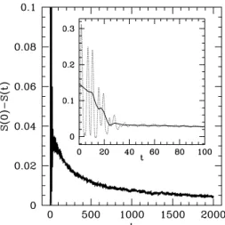
Finally, we introduce a measure of the partitioning of the kinetic energyΠ(t), which we use to describe the
nonequilib-FIG. 2: Number of oscillons nucleated between t and t+δt at T=0.22 andδt=1. The global emergence is evident early in the simulations. Inset: probability distribution of radii and periods of oscillations of individual oscillons.
rium evolution of the system: Π(t) =−
d2k p(k,t)lnp(k,t), (4) where p(k,t) =K(k,t)/
d2kK(k,t), andK(k,t) is the ki-netic energy of the k-th mode. Π(t) attains its maximum (Πmax=ln(N)on a lattice withNdegrees of freedom) when equipartition is satisfied. This occurs both at the initial ther-malization(t =0)and final equilibrium states, since in this case all modes carry the same fractional kinetic energy. In Fig. 3 we show the change ofΠ(t) from the initial state, Π(t=0)−Π(t), for the closed system atT =0.22. At late times (t>150), we have found that the system equilibrates exponentially in a time-scaleτ≃500. At early times, the localization of energy at lower k-modes, corresponding to the global emergence of oscillons, prolongs this approach to equipartition. The inset of Fig. 3 shows the large variations inΠ(t)(dotted line) that arise due to the synchronous oscilla-tions in the kinetic energy of these configuraoscilla-tions. Also shown (solid line) is the average between successive peaks ofΠ(t), with a plateau at approximately 20<t<70 that coincides with the maximum oscillon presence in the system. Thus, oscillon configurations serve as early bottlenecks to equipar-tition, temporarily suppressing the diffusion of energy from low (0<|k| ≤0.8) to higher modes.
IV. QUENCHING INTO ASYMMETRIC DOUBLE WELLS: RESONANT NUCLEATION
Forα>αc=1.5 the potential is asymmetric with the mini-mum atφ=0 becoming metastable. We proceed as before by quenching the system from a single well, as illustrated in Fig. 4.
FIG. 3: The change ofΠ(t)from the initial state for closed systems atT=0.22. The exponential approach to equilibrium is clear at late times. The inset illustrates the role of oscillons as a bottleneck to equipartition.
FIG. 4: Schematic picture showing change in potentialV(φ)from single-well to asymmetric double-well after quench.
We have observed that this decay may occur in three possible ways depending on the initial temperatureT and the value of α[12]: i) the transition to the global minimum happens very fast in what can be called a “cross-over” transition; ii) the tran-sition occurs as a single oscillon becomes unstable and grows into a critical bubble. As is well known from the theory of first order phase transitions [8], once a critical nucleus forms it will grow to complete the transition; iii) two or more oscil-lons percolate to become a critical bubble that then grows to complete the transition.
In order to simplify the analysis, we fixed the tempera-ture to be T ≤0.22. From the Hartree potential of Eq. 2, one can see that for large temperatures the potential becomes a single well again. For T ≤0.13 no oscillons are nucle-ated after the quench. In this case, we expect that the usual metastable decay rate based on the theory of homogeneous nu-cleation (HN) will apply, becoming more accurate for smaller T [8, 13]. The decay rate per unit volume obtained from
FIG. 5: The evolution of the order parameterφave(t)atT =0.22 for several values of the asymmetry. From left to right, α =
1.746,1.56,1.542,1.53,1.524,1.521,1.518. The inset showsVefffor the same values.
HN theory is controlled by the Arrhenius exponential sup-pression,Γ(T,α)≃T(d+1)exp[−Eb(T,α)/T], whereEbis the energy of the critical bubble or nucleus andd is the number of spatial dimensions. [We use units wherec=kB==1.] The typical time-scale for the decay in a volumeV is then, τHN≃(VΓ)−1∼exp[Eb(T,α)/T].
In Fig. 5 we show the evolution of the order parameter φave(t)as a function of time for several values of asymme-try, 1.518≤α≤1.746, forT =0.22. Not surprisingly, as α→αc=1.5, the field remains longer in the metastable state, since the nucleation energy barrier Eb →∞ at αc. How-ever, a quick glance at the time axis shows the fast decay time-scale, of order 101−2. For comparison, for 1.518 ≤ α≤1.56, HN would predict nucleation time-scales of order ∼1028≥τHN∼exp[Eb/T]≥1012(in dimensionless units). [The related nucleation barriers with the effective potential are Eb(α=1.518) =14.10 andEb(α=1.56) =5.74.] For small asymmetriesφave(t) displays similar oscillatory behavior to the SDW case before transitioning to the global minimum. Asα is increased the number of oscillations decreases. For large asymmetries,α≥1.746, the entire field crosses over to the global minimum without any nucleation event, resulting in oscillations about the global minimum. This is situation described in case i) above.
In Fig. 6 we show the ensemble-averaged nucleation time-scales for resonant nucleation,τRN, as a function of the nu-cleation barrier (computed with eq. 2), Eb/T, for the tem-peraturesT =0.18, 0.20, and 0.22. [For temperatures above T =0.26 we are in the vicinity of the critical point in which no barrier exists.] The nucleation time was measured when φavecrosses the maximum ofVeff. The best fit is a power law:
τRN∝(Eb/T)B, (5)
FIG. 6: Decay time-scale τRNas a function of critical nucleation effective free-energy barrierEb/T atT=0.18, 0.20, andT =0.22.
The best fits (dashed lines) are power-laws with exponentsB≃3.762, 3.074, and 2.637, respectively.
T, since the synchronous emergence of oscillons becomes less pronounced and eventually vanishes. In these cases we should expect a smooth transition into the exponential time-scales of HN.
We conclude thatfast quenching can dramatically affect the nucleation time-scale of first order phase transitions. In other words, HN fails for fast quenches.
Here we propose the mechanism by which this fast decay occurs: for nearly degenerate potentials,αc<α≤αI, the crit-ical nucleus has a much larger radius than a typcrit-ical oscillon; it will appear as two or more oscillons coalesce. We call this Re-gion I, defined forRb≥2Rosc, whereRoscis the minimum os-cillon radius computed from Ref. [5]. Figure 7 illustrates this mechanism. Two oscillons, labeled A and B, join to become a critical nucleus. [The interested reader can see simulation movies at http://www.dartmouth.edu/∼cosmos/oscillons.]
Asαis increased further, the radius of the critical nucleus decreases, approaching that of an oscillon. In this case, a sin-gle oscillon grows unstable to become the critical nucleus pro-moting the fast decay of the metastable state: there is no co-alescence. We call this Region II,αI<α≤αII,Rb<2Rosc. This explains the small number of oscillations onφave(t)as αis increased [cf. Fig. 5]. To corroborate our argument, in Fig. 8 we contrast the critical nucleation radius with that of oscillons as obtained in Ref. [5], for different values of effec-tive energy barrier and related values ofαatT =0.22. The critical nucleus radiusRbis equal to 2Roscforα=1.547. This defines the boundary between Regions I and II: forα≥αIa single oscillon may grow into a critical bubble. Finally, for α≥αII=1.746 the field crosses over to the global minimum without any nucleation event.
An obvious extension of the present work is the investiga-tion of “resonant nucleainvestiga-tion” in 3d. Preliminary results in-dicate that the power law behavior persists withB∼1.5 for the relevant range of temperatures for oscillon coalescence. In general, RN will occur whenever the effective potential changes faster than the typical relaxation rate of the longest wavelength of the order parameter. These results could be
ex-FIG. 7: Two oscillons coalesce to form a critical bubble. First two frames from top show oscillons A and B. Third and fourth frames shows A and B coalescing into a critical bubble. Final frame shows growth of bubble expanding into metastable state.
FIG. 8: Radius of critical bubble (Rb) and twice the minimum
ticle physics: the inflaton was to be the same scalar field pro-moting the symmetry breaking of Grand Unified models, link-ing early-Universe cosmology to high-energy particle physics. In fact, it is this particle physics connection that motivated and motivates the widespread use of scalar fields in early-Universe physics.
Unfortunately, Guth’s original proposal didn’t work. As he himself argued, and then Linde, and Albrecht and Steinhardt[17], the bubble-nucleation rate could not compete with the exponential expansion rate of the Universe: the tran-sition would never end. Roughly, while bubble walls ex-panded with the speed of light, their centers receded from each other exponentially fast, making it impossible for the walls to touch, the bubbles to coalesce, and the transition to complete. Old Inflation gave rise to a universe with inhomo-geneities incompatible with the observed smoothness of the cosmic microwave background[18]. Guth and Weinberg[19], and later Turner, Weinberg, and Widrow[20], performed a de-tailed analysis of the constraints needed to render OI and OI-inspired scenarios viable. They concluded that a strong (or, equivalently, slow) first order phase transition based on a sin-gle scalar field could not be made to work: the ratio of decay rate to the expansion rate per unit volume [H4≃(T2/MPl)4], had to be sufficiently small
ε≡Γ/H4≤10−4, (6)
initially, so that early bubbles didn’t produce inhomo-geneities during nucleosynthesis and on the CMB. (ForΓ≃ T4exp[−E(T)/T] and TGUT =1015 GeV, this implies that E(T)/T 46.1 initially). On the other hand, it had also to grow by the end of inflation (ε→9π/4) to guarantee that the transition was completed[20]. [This impliesE(T)/T 34.9.] In other words, successful inflation forced the decay rate to be time-dependent: small at the beginning of inflation and of order unity at the end. As further work has shown, this could be achieved by invoking more fields[21] and/or a nonminimal gravitational coupling[22].
Given what we have learned in the previous section about resonant nucleation, it is natural to wonder whether such effects can play a role on inflation. If we write εHN ≃ T4exp[−E(T)/T] to represent the ratio of eq. 6 using the homogeneous nucleation rate, andεRN ≃T4[E(T)/T]−Bthe ratio using the RN rate, equality is attained whenever
B=β/lnβ, (7)
FIG. 9: Comparison of homogeneous nucleation (HN) and resonant nucleation (RN) with powerBin an expanding Universe. For a fixed B and nucleation barrierβ=E(T)/T (orSbatT =0), the line
de-notes equality. Values above the curve imply faster HN, while those below imply faster RN.
whereβ≡E(T)/T (or≡SbatT =0). In Fig. 9,Bis shown for representative values of the nucleation barrierβ. The line denotesεHN/εRN=1. The squares denote the limits imposed by the inflationary constraints of Ref. [20]. For these values ofβ, unlessB9, which is very unlikely, resonant nucleation rates are always faster. Ind=2, whereB≃3, it is clear that εHN/εRN<1 for all realistic values ofβ, not a surprising re-sult.
Why is this useful for inflation? For successful inflation with HN, the constraints of Ref. [20] limit the nucleation bar-rierβ to be fairly small O(∼40). [See Fig. 9.] However, calculations of bounce actions show thatβusually scales with inverse powers of coupling constants. These two requirements compete with each other, making it hard to have small nucle-ation barriers with small couplings. Applying the percolnucle-ation constraint to the RN rate, one obtainsβB∼1016. ForB=3, this givesβ∼1016/3: small couplings (or, equivalently, large barriers) are easier to accommodate with RN, the first reason why it may be useful for inflation.
potential[21]:
V(φ,ψ) = 1 4λ
M2−λψ22+m2 2 φ
2+g2 2 φ
2ψ2. (8)
Inflation is driven by the energy densityV(φ,0)while the in-flaton (φ)is rolling down along theψ=0 valley[16]. As φ reaches a critical value,ψ becomes spinodally unstable and quickly rolls to one of the minima (or both, but this creates do-main walls, another problem), terminating inflation abruptly.
The key difference with the mechanism being proposed here is that bubble nucleation still occurs at the end of in-flation. A possible name is henceresonant inflation(RI): it blends OI with the physics of resonant nucleation.
Modify the potential for the fieldφthat gives rise to RN by coupling another field (ψ) quadratically to it as follows,
V(φ,ψ) = 1 2
m2+g2ψ2 φ2
−α 3φ
3+λ 8φ
4+
+1 2m
2
ψψ2+|V(φ+,0)|, (9)
whereφ+is the value ofφat the global minimum ofV(φ,0)
so thatV(0,ψ)provides the net vacuum energy responsible for inflation. [Note that here the inflaton isψ.] Inflation lasts whileψis rolling down theφ=0 valley. Notice that the mass term for φ,M2φ=m2+g2ψ2, decreases as ψrolls down its potential. While M2φ>α2/2λ, the only minimum in the φ direction is atφ=0. However, asψdecreases,Mφ2will even-tually drop belowα2/2λand a new minimum will appear at φ+=αλ 1+ (1−2Mφ2λ/α2)1/2
. AtMφ2=49αλ2, the two min-ima are degenerate. At this point, asψcontinues to approach zero, the minimum atφ=0 becomes metastable. Oscillations inφ, induced by the decrease in its mass, will induce RN. This will be true as long as the decrease inMφ, ˙Mφ≃g
2
mψψ, is fast˙ enough. [It was assumed for simplicity that g2ψ2/m2≪1 which is not true for very smallψ.]
For RI to work, ˙Mφ/Mφ<Hduring inflation and ˙Mφ/Mφ> H after it. During inflation, with a slow-roll approximation, ψψ˙ ≃ −m
2
ψ
3Hψ2. We then obtain, ˙
Mφ≃ −g2 m2ψ 3Hmψ
2. (10)
Also, ifNis the number ofe-folds,ψ2
e=ψ2i − M2Pl
2πN, where
ψi(e)is the value of the fieldψat the beginning (end) of the
inflationary period. [For simplicity, it was assumed that dur-ing inflation 12m2ψψ2>|V(φ
+,0)|, that is, inflation is
domi-nated initially by the vacuum energy of the inflaton fieldψ.] Slow-roll ends whenψ2
eMPl2/12π. Using this result and eq. 10, the slow variation ofMφimplies,g2(12π)1/2<(m/MPl)2. [Form∼1016GeV,g<4×10⁻⁴.] This condition is also con-sistent with the approximationg2ψ2/m2≪1 forψ
i>ψ>ψe, that is, during inflation.
If slow-roll ends when the minimum in φ+ appears, we
obtain (this is similar to the critical condition in hybrid inflation[21]),
α2 0 2λ =1+
g2MPl2
12πm2 , (11)
where we defined for convenienceα≡mα0. The condition for slow variation of Mφ during inflation forces the second term on the rhs of eq. 11 to be very small. Thus, if we want to impose that theφ+ minimum appears close to the end of
inflation, we must haveα2
0/2λ∼1, not a difficult condition to satisfy.
As inflation ends,ψwill start rolling down fast towards the ψ=0 minimum and oscillate around it. Since in this regime,
˙
Mφ/Mφ∼(g2/m2)ψψ, the rapid motion of˙ ψwill induce the
time-dependence inMφneeded to trigger resonant bubble
nu-cleation. In order for the transition to end successfully, the percolation constraint εRN >9/4π, must be satisfied. This implies,
(Sb)B< 4π 9 M Pl m 4 . (12)
Ifm∼1016GeV andB∼2 (as indicated by preliminary re-sults ind=3), RI terminates efficiently ifSb106. Since the inflationary phase is due to the slow-roll dynamics of the ψfield and not by the metastable fieldφ, the percolation con-straint can be satisfied by a wide range of couplings. Also, sinceφ=0 only becomes metastable afterthe end of slow roll, there is no need to impose the big bubble constraint: once ψstarts rolling fast at the end of inflation, RN will ensue and rapid bubble nucleation and coalescence will quickly reheat the Universe. Although several details remain to be worked out, this preliminary analysis indicates that resonant nucle-ation can be successfully applied to inflnucle-ationary cosmology.
The author would like to thank the organizers for their kind hospitality.
[1] A. Einstein, Ann. Phys.17, 549 (1905).
[2] P. H¨anggi and F. Marchesoni, “100 Years of Brownian Motion,” submitted to Chaos, [cond-mat/0502053].
[3] D. Walgraef, Spatio-Temporal Pattern Formation Springer, New York, 1997; M. C. Cross and P. C. Hohenberg, Rev. Mod. Phys.65, 851 (1993).
[4] A. Vilenkin and E. P. S. Shellard, Cosmic Strings and Other
Topological Defects, Cambridge University Press, Cambridge, 1994.
[5] M. Gleiser, Phys. Lett. B600, 126 (2004).
[6] M. Gleiser, Int. J. Mod. Phys. D, in press [hep-th/0602187]. [7] G. Aarts, G. F. Bonini, and C. Wetterich, Phys. Rev. D 63,
[13] S. Coleman, Phys. Rev. D15, 2929 (1977); C. Callan and S. Coleman, Phys. Rev. D16, 1762 (1977); A. Linde, Nucl. Phys. B216, 421 (1983); [Erratum: B223, 544 (1983)]