Data Centric Sensor Stream Reduction for Real-Time Applications in Wireless Sensor Networks

(1)

OPEN ACCESS

sensors

ISSN 1424-8220

www.mdpi.com/journal/sensors

Article

Data Centric Sensor Stream Reduction for Real-Time

Applications in Wireless Sensor Networks

Andre Luiz Lins Aquino1,⋆and Eduardo Freire Nakamura2

1 _{Computer Science Department, Federal University of Ouro Preto, Ouro Preto, MG, Brazil}

2 _{FUCAPI – Analysis, Research and Technological Innovation Center, Manaus, AM, Brazil;}

E-Mail: eduardo.nakamura@fucapi.br

⋆ _{Author to whom correspondence should be addressed; E-Mail: alla@iceb.ufop.br;}

Tel.: +55–3559–1692.

Received: 13 October 2009; in revised form: 9 November 2009 / Accepted: 13 November 2009 / Published: 2 December 2009

Abstract: This work presents a data-centric strategy to meet deadlines in soft real-time applications in wireless sensor networks. This strategy considers three main aspects: (i) The design of real-time application to obtain the minimum deadlines; (ii) An analytic model to estimate the ideal sample size used by data-reduction algorithms; and (iii) Two data-centric stream-based sampling algorithms to perform data reduction whenever necessary. Simulation results show that our data-centric strategies meet deadlines without loosing data representativeness.

Keywords: sensor-stream reduction algorithms; wireless sensor network; data-centric routing algorithm

1. Introduction

(2)

is not controllable, applications usually use probabilistic models to process data, and communication does not have acknowledgment.

By considering the real-time applications in WSNs, we can identify some related work. In general, current contributions consider architectures and mathematical models for general applications [4–6]. Aquino et al. [7] propose and evaluate a design strategy to determine minimum deadlines used by a specific stream reduction algorithm in general WSNs applications. However, routing and application-level solutions for specific real-time scenarios have been recently proposed [8–10].

In WSNs applications, physical variables, such as temperature and luminosity, can be monitored continuously along the network operation. The data set representing these physical variables can be referred to asdata-stream[11]—orsensor-stream, considering the WSNs context. As a consequence of this continuous monitoring, we might have high delays in such a way that real-time deadlines are not met. This motivation led us to propose a strategy to control the amount of data gathered by the network and its associated delay.

Before introducing our data-centric strategy, allow us to comment on data-stream related work. The data-stream contributions usually focus either in improving stream algorithms [12–15] or in applying the data-stream techniques to specific scenarios [16–20]. However, regarding data-stream solutions used in WSNs, we can identify a few researches that consider WSNs as distributed databases in which some functions (e.g., maximum, minimum and average) can be computed in a distributed fashion [21–25].

Considering real-time requirements and sensor-stream characteristics, we propose a data-centric strategy capable of reducing the data during data routing. In this case, the routing elements consider some application aspects, such as data type and deadline information. Our strategy considers: (1) a project design of real-time application to obtain the minimum deadlines; (2) an analytic model to estimate the ideal sample size used by the reduction algorithms; (3) and two stream-based sampling algorithms to perform data reduction when necessary during the routing task.

To validate our data-centric strategy, we use specific scenarios in which application deadlines cannot be met without data reduction. In our simulation, we use a naive tree routing based on shortest-path tree in a flat network. Application information is fed to relay nodes during build and rebuild tree phases. To identify the stream item delay, we consider that the clocks of the nodes are exactly synchronized. Thus, the time synchronization problem in WSNs [26] is not considered here. However, data quality is evaluated to show the associated data reduction impact. Simulation results show that our data-centric strategies meet deadlines without loosing data representativeness.

(3)

Our contribution can be highlighted through the analytical model, project design, different sample stream algorithm, and evaluation considering three more realistic real-time scenarios. The general contributions of our strategy are the following:

• Data-stream: In this work, we use sensor-stream algorithms as an in-network solution, and we improve the network performance by reducing the packet delay in real-time applications.

• Data reduction: Regarding data reduction, we show that we can meet real-time application deadlines when we use sensor-stream techniques during the routing task. This in-network approach represents a new contribution.

• Real-time: We present a analytical model to estimate the ideal amount of data-reduction, and we apply the stream-based solution in realistic real-time scenarios. To the best of our knowledge this is the first work that tries to quantify the reduction intensity based on real-time deadlines.

This work is organized as follows. Section2. presents the data-centric real-time reduction problem. Section 3. shows how to design real-time sensor network applications by using stream-based data reduction. Section 4. discusses a formal formulation that is used to determine the ideal sample size. Section 5. describes the sampling stream reduction algorithms. Simulation results are presented in Section6., and Section7. presents our conclusions and outlook.

2. Problem Statement

The problem we address in this work is the sensor-stream reduction algorithms as a data-centric mechanism to meet deadlines in real-time applications. We consider the data-stream sampling technique to perform data reduction [36]. Since we use a sensor-stream algorithm for data reduction, the scope, and the problem itself can be defined as follows.

Let us consider a WSN monitoring physical or environmental conditions, such as temperature, sound, vibration, pressure, motion or pollutants, at different locations. Such a system is represented by the diagram [37]:

N V∗ _V _V′

D∗ _D _D′

w

P

u

R∗

w

S

w

Ψ

u

R

u

R′

This diagram illustrates the following behavior:

• The ideal behavior denoted by N → V∗ _→ _D∗_{, where} _N _{denotes the environment and the}

process to be measured, P is the phenomenon of interest, withV∗ _{their space-temporal domain.}

If complete and uncorrupted observation was possible, we could devise a set of ideal rules R∗

leading to ideal decisionsD∗_.

(4)

information, we can conceive the set of rulesRleading to the set of decisionsD. We considerV

to be a sensor-stream, due to its “time series” characteristics.

• The reduced behavior is denoted byN → V∗ _→ V _→ V′ _→ _D′_{. Dealing with}V _{may be too}

expensive in terms of, for instance, power, bandwidth, computer resources usage, and, specially, time delivery to meet the deadline requirements. Since the level of redundancy is not negligible in most situations, we can reduce this information volume. Sensor-stream reduction techniques are denoted byΨ_{, and they transform the complete domain}V_{into the smaller one}V′_{. New rules that}

useV′ _{are denoted by}_R′_{, and they lead to the set of decisions}_D′_.

Based on these behaviors, the problem addressed in this work can be stated as follows:

Problem definition: Given a sensor-stream behavior, how can we use a data-centric data reduction algorithm (Ψ_{) to meet application deadlines? Moreover, what is the impact over the decisions}_{D, when} we use theΨ_{reduction over}V_{generated by}_S?

To address the data-centric reduction problem in real-time applications, we consider the following assumptions:

• WSN topology: The set of sensorsS = (S1, . . . , Sn)is distributed in a squared areaA =L×L. There is only one sink node located at(0,0)on the left bottom corner. The density is kept constant and all nodes have the same hardware configuration.

• Routing protocol: The network communication is based on a multihop shortest-path tree [38] as the routing protocol. To evaluate only the data-centric stream reduction performance, the tree is built just once before the traffic starts and the network is kept static. The build tree process is depict in Figure 1. First in(a), the sink node sends a flooding message requesting to build tree. After this, in(b), the nodes sets your father node considering the first message received in flooding process (it is considered that the first packet received represents the shortest path to sink). Finally, in(c), we have the complete tree mounted.

• Sensor-stream item: V_i _{values are generated by one specific sensor located at} ₍_{L, L}₎ _{on the}

right top corner (the opposite side of sink node), for convention we useV_{to represent the stream}

generated. For each stream, we process one stream item V ₌ _{V_{1, . . . ,}V_n_} _{where the amount}

of data stored before the data sent is |V_| ₌ _n_{. The generation is continuous at regular intervals}

(periods) of time. We consider gaussian data (µ= 0.5andσ = 0.1) sent in bursts.

• Quality of a sample: To assess the impact of data reduction on data quality, based on decision

D, we consider two rules: Rdst and Rval. The rule Rdst aims at identifying whether V

and V′ _{data distributions are similar. To compute this distribution similarity (}_Υ_{), we use the}

Kolmogorov-Smirnov test [39]. The rule Rval evaluates the discrepancy among the values in sampled streams,i.e., if they still represent the original stream. To quantify this discrepancy (Φ_),

we compute the absolute value of the largest distance between the average value of the original data, and the lower or higher confidence interval values (95%) of the sampled data:

(5)

in which the pair (vlow; vhig) is the confidence interval for the sampled data andavggis the average (mean value) of original data [36]. These rules help us to identify the scenarios where our sampling algorithm is better than simple random sampling strategy.

Figure 1. Build tree process.

Sink

(a) Build request.

Sink

(b) First packet received.

Sink

(c) Tree mounted.

These assumptions are considered in the whole paper. For instance, the routing algorithm is shortest path tree, the stream item is the set V ₌ _{V₁_{, . . . ,}V_n_}_{, and so on.} _{In the next three}

sections, we answer the questions addressed in Problem definition by presenting the reduction design in real-time applications, the analytic model that estimate the ideal sample size|V′_|_{, and the data-centric}

reduction algorithms.

3. Data-Centric Reduction Design in Real-Time WSNs Applications

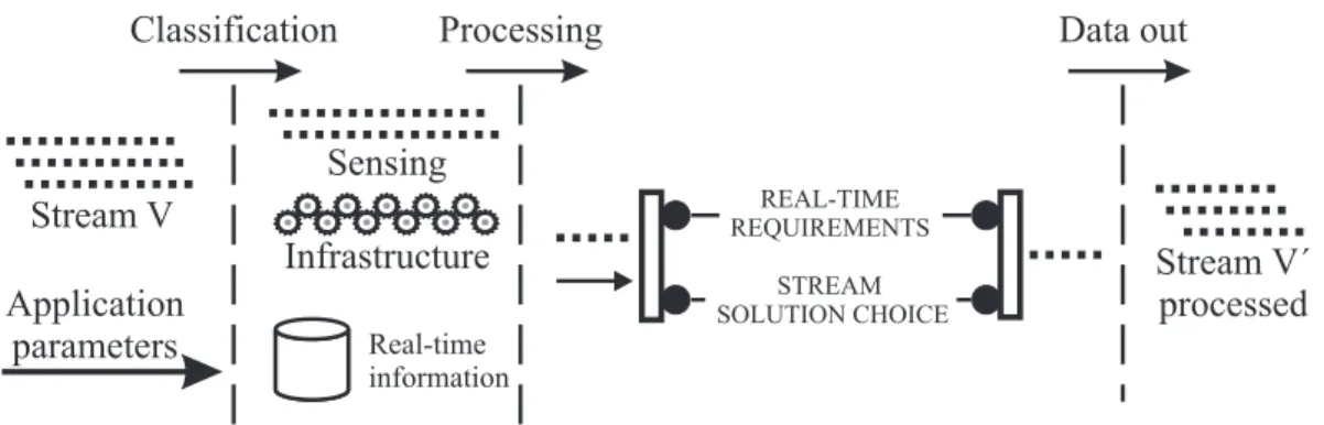
The first task of our data-centric strategy considers the design of real-time application. The objectives of this design are the: characterization of the stream flow while it passes by each sensor node; identification of the software components required by real-time applications by each sensor node; and identification of the required hardware resources by each sensor node. These aspects are illustrated in Figure2, which shows the data-centric design in real-time WSNs applications, this design represents the sensor node view.

Figure 2. Data-centric reduction design in WSNs real-time application, the sensor view.

Stream V´ processed Processing

Stream V

Application parameters

Sensing

Infrastructure

Real-time information

REAL-TIME REQUIREMENTS

STREAM SOLUTION CHOICE

Classification Data out

Basically, we have three steps to characterize the stream flow in each node: received data, data classification, and data processing. Considering the received data,V_{can be generated by the application}

or received from other nodes. In both cases,V_{is delivered to the routing layer.} _{Application parameters}_,

(6)

node receives V_{, we need to classify its type (classification step). In our case, the types considered}

are the sensing received from the application and the infrastructure received from other nodes. This classification is important because the routing layer behavior will be different for each one. When the node receives theapplication parameters, thereal-time informationdatabase must be updated with new information. Such information include, for example, application deadlines, hops towards the sink, and time towards the sink. In the processing step, real-time requirementsare verified. These requirements are used to decide the more suitable reduction strategy (stream solution choice), it is important highlight that this requirements are dynamically updated when the stream is received,i.e., the relay node has only the local information. This occurs because the reduction may lead to different outputs with different “data qualities”. In our case, in this step, we determine|V′_|_{according to the deadline requirements. The}

sample size determination and the reduction algorithm will be presented latter on. Finally, in the data out step,V′_{, which may be reduced, is routed towards the sink.}

In Figure 2, we can identify the software components required in real-time applications: a classification component to identify the type of |V_|_{; an application-parameter component to process}

and store real-time application parameters; an oracle component to verify when the current stream item requires reduction; a stream size estimation component to compute |V′_|_{, when necessary; a reduction}

component to perform the reduction; and a data out component to set the new parameters aggregated toV′_.

Finally, the hardware resources necessary must be identified considering the |V_| _{supported and the}

reduction algorithm complexity. |V_|_and_|V′_|_{are used to estimate the memory and bandwidth necessary}

to conceive the real-time WSN solution. In addition, the complexity of the reduction algorithm is important to determine the computational power necessary to apply the reduction strategy. These aspects are important to conceive a successful data-centric reduction for real-time applications.

4. What Is the Ideal Sample Size?

The second task of our data-centric strategy considers the |V′_| _{estimation. The objectives of this}

estimation is to allow relay nodes to perform the reduction in a data-centric way, i.e., the routing layer uses application information to meet real-time requirements by applyingΨ_{to reduce}_|V_|_.

In the stream solution choice of processing step (Figure 2) we determine |V′_| _{necessary to meet}

the deadline specified in real-time requirements. In this case, to determine |V′_|_{, every sensor node}

has a maximum packet size (ps) permitted. In our case, we consider ps = 20items. However, every relay node knows its hop and time distances (considering only one packet) to the sink node, hdst

and tdst respectively. This information is fed during the tree building phase, and stored in real-time informationdatabase.

In some cases,V_{needs to be fragmented in}V₌_{V1_{. . .}Vnf}_{, where}nf _{is the number of fragments.}

All Vj₍₀ _{< j} _≤ _nf₎ _{encapsulate the application deadline (}_da_{), number of fragments (}_nf_{), instant the}

fragment was generated (tgen), and its number of hops (hsrc). Thus, the relay node has all information about the stream item when it receives only one fragment.

(7)

Sink Source Relay

Time line

tSRC

dL

This deadline accounts the route between the relay and the sink node, and it is defined as

dl =da−tsrc

wheretsrc is the estimated time to deliverVj _{from the source node to the current relay node,}

tsrc =tnow−tgen

Let us considertsrc be the time of theV1_{to travel from source at relay node. Then,}V2_{will arrive in} tsrc/hsrc units of time (e.g., seconds),i.e., estimated time for the last hop as depicted at the following:

Sink Source Relay

Time line

tSRC tSRC/hSRC

This consideration is necessary, because the information in the relay node is only about tsrc, therefore, the complete stream cames from the last relay node rather than directly from source. Thus, the estimated time receiveV_is

trec = (nf −1)tsrc/hsrc (1)

In a similar way, let us considertdst the time of theV1 _{to travel from relay node at sink. Then,} V2

will arrive in tdst/hdst units of time (e.g., seconds), i.e., estimated time for the last hop as depicted at the following:

Sink Source Relay

Time line

tDST tDST/hDST

Thus, the estimated time to deliverV_is

tdel =tdst+ (nf −1)tdst/hdst (2)

The first term of the sum is considered in tdel equation because V1 _{has not arrived yet. Remember}

(8)

Thus,|V′_|_{is determined and used only if the}_{gap >}₀_,_i.e._{, there is time to deliver the complete stream}

or part of it. gapis defined as

gap=dl−delay (3)

where the streamdelayat the sink node is

delay =trec +tdel (4)

The delay can be depicted as the following:

Sink Source Relay

Time line

tDST delay

tSRC

Thus, to compute|V′_|_{, used to meet the application deadline, we consider the inequality}

gap >0 (5)

from (3) and (4) we have

dl−delay >0

dl−(trec+tdel)>0

using (1) and (2) we have

dl−((nf −1)tsrc/hsrc+tdst+ (nf −1)tdst/hdst)>0

so that

nf <1 + hsrchdst(dl−tdst)

hdsttsrc+hsrctdst

considering thatnf =⌈|V′_|_/ps_⌉_{, we have}

|V′_|_{< ps} µ

1 + hsrchdst(dl−tdst)

hdsttsrc+hsrctdst ¶

finally to reach the inequality we have

|V′_|₌_ps µ

1 + hsrchdst(dl−tdst)

hdsttsrc+hsrctdst ¶

−1 (6)

Meanwhile, considering the |V′_| _{presented by Aquino} _{et al.} _[₄₀_{], the sample size is estimated}

based on

|V′_|₌_ps_da/tdst ₍₇₎

In order to identify both formulations, in simulation study (Section6.), we will use the termscomplex formulation andsimplified formulation to represent Equations 6and 7, respectively. However, in both cases when thegap ≤ 0we consider|V′_| ₌_ps_{or the received is simple forwarded to preserve the data}

(9)

5. Sensor-Stream Reduction

Finally, the third aspect of our data-centric strategy considers the sensor-stream reduction algorithm (Ψ_{). The objective of this reduction is to try to meet deadlines from real-time applications while keeping}

data fidelity (accuracy). The proposed sensor-stream reduction is motivated by the problem stated in Section2. and evaluated in processing phase of project design described in Section3.

The in-network (data-centric) reduction algorithm is integrated into a shortest-path routing tree. In this case, the routing tree is built, based on application requirements, from the sink (root) to the sources nodes by using a flooding strategy. In this flooding, hdst andtdst values are delivered to every sensor node. Once the routing tree is built, the source node can sendV_{towards the sink. At this moment, relay}

nodes receive {V1_{. . .}Vnf}_{in some packets (fragments) and forward them to another relay node until}

the sink is reached.

In this forward process, when a relay node receivesV1_{, it checks the stream reduction criterion, in}

our case ifgap > 0(Equation5). If the criterion is satisfied V1 _{is stored and the node waits to receive}

and store {V2_{. . .}Vnf}_{. Otherwise, all fragments are forwarded. It is important highlighted that this}

forwarding is in routing layer, considering the sensor radio, certainly, the fragments are queued until the sender radio turns able. Based on thereal-time information,|V′_|_{is computed through Equation}₆_{. When}

all fragments arrive, theΨ_{reduction is enabled. This forwarding process is shown in Algorithm}₁_.

Algorithm 1: Pseudo-code of reduction decision.

Data:Vj _{– fragment stream received}

begin

1

“Get fromVj _{the fragments information”}

2

ifj= 1then

3

“gapis computed through equations (2–4)”

4

ifgap >0then

5

“EnableV_storage”

6

|V′_|₌_p s

³

1 +hsrchdst(dl−tdst) hdsttsrc+hsrctdst ´

−1{Equation6}

7

end

8

end

9

ifStorage is enabledthen

10

“StoreVj_”

11

ifj =nf then

12

V′ _←_“ComputeΨ_onV_with_|V′_|_size”

13

“SendV′_”

14 end 15 end 16 else 17

“ForwardVj_”

18

end

19

end

(10)

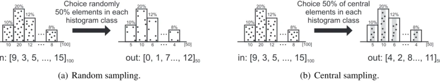
When the reduction is able, a histogram ofV_{is built (line 13 of Algorithm}₁_{). We consider a simple}

histogram, all elements sensed are between [0; 1] and we have 10equals histogram classes. To obtain such a sample, we choose the central elements of each histogram class, respecting the sample size |V′_| _{and the class frequencies of the histogram. Thus, the resulting sample will be represented by the}

same histogram. Meanwhile, considering the sensor-stream reduction algorithm presented by Aquino

et al.[40], the sample elements are randomly chosen in each histogram class instead of considering the central elements. The reduction algorithms, used here, and their operations are depicted in Figure 3. The random sampling(a), we have a “stream inV_{” with}₁₀₀ _elements,_|V′_{| →} _50%_ofV _{is randomly}

chosen (this choice is performed in each histogram class), and then a “stream outV′_{” is generated with}

|V′_|_{= 50}_{. The central sampling}_(b)_{, we have again a “stream in}_V_{” with}₁₀₀_elements,_|_V′_{| →} _50%_of V_{is choice considering the central histogram classes elements, and then a “stream out}V′_{” is generated}

with|V′_|_{= 50}_.

Figure 3. Reduction algorithms.

in: [9, 3, 5, ..., 15]100 out: [0, 1, 7..., 12]50

Choice randomly 50% elements in each

histogram class 8 ... 10% 20% 12% 8% 12 20

10 ... [100] 4

... 10% 20% 12% 8% 6 10

5 ... [50]

(a) Random sampling.

in: [9, 3, 5, ..., 15]100 out: [4, 2, 8..., 11]50

Choice 50% of central elements in each

histogram class 8 ... 10% 20% 12% 8% 12 20

10 ... [100] 4

... 10% 20% 12% 8% 6 10

5 ... [50]

(b) Central sampling.

In order to identify both algorithms, in simulation study (Section6.), we useΨ_central_andΨ_random _to

represent the central and random elements choice, respectively. TheΨ_central_{sample reduction process is}

present in Algorithm2.

Analyzing the Algorithm2we have:

Line 2 Executes inO(|V_| _log_|V_|₎_;

Lines 11–15 Define the inner loop that determines the number of elements at each histogram class of the resulting sample, consideringHcn as the number of histogram class and n′

coli as the columns

in sampled histograms, where0< i ≤ Hcn. ThePHcn

i n′coli =|V

′_|_{, we have that this inner loop}

executes inO(|V′_|₎_steps.

Lines 7–20 Define the outer loop in which the input data is read and the sample elements are chosen. Because the inner loop is executed only when condition in line 8 is satisfied, the overall complexity of the outer loop is O(|V_|_{) +}_O₍_|V′_|_{) =} _O₍_|_V_|₊_|_V′_|₎_{, since we have an interleaved execution.}

Letncoli be the columns in original histograms, where0< i ≤Hcn. Basically, before evaluating

the condition of Line 8, ncoli is accounted and |V|/Hcn interactions are executed. Whenever

this condition is satisfied, n′

coli is built and|V

′_|_/Hcn _{interactions are executed (Lines 11–15). In}

order to build the complete histogram, we must cover all classes (Hcn), then we haveHcn(|V_|₊

|V′_|₎_/Hcn ₌_|_V_|₊_|_V′_|_.

(11)

Thus, the overall complexity is

O(|V_| _log_|V_|_{) +}_O₍_|V_|₊_|V′_|_{) +}_O₍_|_V′_| _log_|_V′_|_{) =}_O₍_|_V_| _log_|_V_|₎

since |V′_{| ≤ |}V_|_{. The sorting step is necessary, because, in our case, to build the histogram, we need}

the elements to be sorted, so that we always get the correct elements of V′_{. The space complexity is} O(|V_|₊_|V′_|_{) =} _O₍_|_V_|₎_{because we store the original sensor-stream and the resulting sample. Since}

every source node sends its sample stream towards the sink, the communication complexity isO(|V′_|_D₎_,

whereDis the largest route (in hops) in the network.

Algorithm 2: Pseudo-code ofΨ_central_{sampling reduction.} Data:V_{– original sensor-stream}

Data:|V′_|_{– resulting sample size} Result:V′ _{– resulting sample set} begin

1

Sort(V₎

2

wid←“Histogram’s class width”

3

f st←0{first index of histogram class}

4

ncol ←0{number of elements per columns inV}

5

w←0

6

fork←0to|V_{| −}₁_do

7

ifV_[_k_]_>V_[_{f st}_{] +}_widor_k₌|V_{| −}₁_then

8

n′

col← ⌈ncol|V′|/|V|⌉ {number of elements per columns inV′}

9

index←f st+⌈(ncol−n′_col)/2⌉

10

forl←0ton′ coldo

11

V′_[_w_]_←V_[_index_]

12

w←w+ 1

13

index←nextIndex

14

end

15

ncol←0

16

f st←k

17

end

18

ncol ←ncol+ 1

19

end

20

Sort(V′₎_{{according to the original order}}

21

end

22

6. Simulation

(12)

To identify assess the network behavior, we variate the number of nodes and the stream size (|V_|_).

The evaluated parameters are the delay and error in data quality, specified by two statistical tests. The default parameters used in simulations are presented in Table1.

To evaluate the delay in real-time scenarios, it is important to determine the minimum deadline (dmin) for each number of nodes and |V_| _{being considered. To do this, we consider different network sizes}

(128,256,512, and1024), the|V_|₌_{₂₅₆_,₅₁₂_,₁₀₂₄_,₂₀₄₈_}_{, and only one data source generating}V_{. In}

our case, the dmin values is determined by measuring the time between the first data packet sent by the source and the last packet received by the sink, i.e., the time for V _{to be entirely received by the sink.}

Figure4illustratesdminvalues for all scenarios being considered.

Table 1. Simulation parameters.

Parameter Values

Network size Varied with density

Queue size Varied with stream

Simulation time (seconds) 1100 Stream periodicity (seconds) 10

Radio range (meters) 50

Bandwidth (kbps) 250

Initial energy (Joules) 1000

Figure 4. Minimum deadlines.

256 512 1024 2048

Delay

Amount of data generated at the source node

Packet delay (s)

0

5

10

15

20

128 nodes 256 nodes 512 nodes 1024 nodes

It is important to highlight that if either application has a deadline smaller than the one shown in Figure 4 or the network is not in perfect conditions, then all data cannot be transmitted unless some reduction is performed. However, despite all nodes (sources) know the real time requirements of the packets they generate, they cannot infer the necessary data reduction locally because the network has some global restriction not perceived for them.

(13)

based on decisionD, we consider the rulesRdstandRval defined before. These rules are represented by

Υ_andΦ_{errors, respectively.}

It is possible to apply these rules, because we consider the reduction of only one source, i.e., our sampling is performed in each data set separately. For example, considering a simple network of nodes connected as a tree as Sink–NodeA–NodeB. After in network data reduction we give equal opportunity

to the data points ofNodeAandNodeBseparately. So, clearly the data gathered in the sink will represent

the original data of the network, where neither data nodes will be over-represented.

The deadlines for the real-time scenarios, that we consider, are 50% of the minimum deadlines with(out) concurrent traffic; minimum deadlines with delay caused by relay nodes in each packet transmitted with(out) concurrent traffic. These study are discussed in the next subsections. For all scenarios, we evaluate the simplified and complex formulations, both usingΨ_central_orΨ_random_{. We use}

a Monte Carlo simulation [41] considering a complete mapping between the number of nodes and the stream size, only unusual results will be presented. However, the y-axis scale is not kept constant in all figures. The reason is that such a re-scale allow us to make better analysis.

6.1. Half of Deadlines without Concurrent Traffic

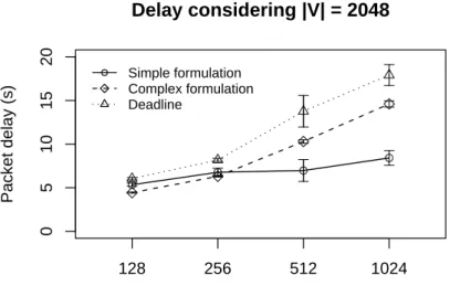
The first scenario considers half of minimum deadlines (da = dmin/2) without concurrent traffic in this case, the application cannot sendV_{and meet}_da_{. In this case,}V_{is reduced by using our data-centric}

strategy. In Monte Carlo simulation, we change the number of nodes (128, 256, 512, and 1024) and |V_| ₍₂₅₆_, ₅₁₂_, ₁₀₂₄_{, and} ₂₀₄₈_{). Figure} ₅ _{shows the delay results varying the number of nodes with}

|V_|_{= 2048}_.

Figure 5. Delay considering the half of deadlines without concurrent traffic.

Delay considering |V| = 2048

Number of nodes

Packet delay (s)

Simple formulation Complex formulation Deadline

128 256 512 1024

0

2

4

6

8

10

(14)

The reason is that, in the simplified formulation, the reduction is harder and less data is forwarded. When the number of nodes is 1024, the simplified formulation delivers19%of data, while the complex formulation delivers25%. This indicates that, considering only the deadline achievement, the simplified formulation is more appropriate. However, the reduction ratio is greater.

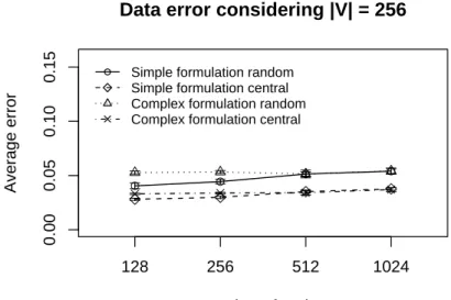
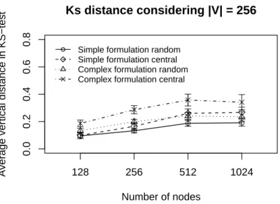
Regarding the data error evaluation. Figures6and7show the error evaluation for different numbers of nodes with |V_| _{= 256}_{. Figure} ₆ _{shows that in all cases we have} Υ _≤ _40%_. Ψ_random_{, in both}

formulations, has a smaller Υ_{-error because the random choice improves data dispersion, and the}

simplified formulation has a smallerΥ_-error.

Figure 6. Υ_{-error considering the half of deadlines without concurrent traffic.}

Ks distance considering |V| = 256

Number of nodes

Average vertical distance in KS−test

Simple formulation random Simple formulation central Complex formulation random Complex formulation central

128 256 512 1024

0.0

0.2

0.4

0.6

0.8

Figure 7. Φ_{-error considering the half of deadlines without concurrent traffic.}

Data error considering |V| = 256

Number of nodes

Average error

128 256 512 1024

0.00

0.05

0.10

(15)

Figure7shows that in all cases we haveΦ_≈_5%_. Ψ_central_{, in both formulation, has a smaller}Φ_-error

because the central elements choice improves the average test. Again, the simplified formulation has a smallerΦ_{-error. The error evaluation indicates that the simplified formulation is more appropriate in}

this specific scenario. Considering the evaluated algorithms,Ψ_random_{may be used when}_Rdst _{is the rule}

priority, otherwise,Ψ_central_{should be used.}

The partial conclusion, considering this critical real-time scenarios, is that the simplified formulation is more appropriate, because the deadlines are usually met while keeping data representativeness. Considering the sampling algorithm, Ψ_random _or Ψ_central _{can be used when data application decisions}

are related,RdstorRval, respectively.

6.2. Delay Caused by Relay Nodes without Concurrent Traffic

The second scenario, considersda =dmin and all relay nodes delaying the stream fragments (Vj_{) per} da/10000or0.01%of the da. In this scenario, the application cannot send V_{, because the relay nodes}

eventually can be executing another task, consequently, the deadline da cannot be met. We change the number of nodes (128, 256, 512, and1024) and|V_|₍₂₅₆_, ₅₁₂_, ₁₀₂₄_{, and}₂₀₄₈_{). The objective of this}

scenarios is to identify the appropriate strategy when relay nodes have other high priority tasks.

Figure8shows the delay results when we change the number of nodes with|V_| _{= 2048}_{. In contrast}

to prior scenario, da is always met. The complex formulation, in a more realistic scenario, presents a better time usage, i.e., the delay is closer to deadline values. This occurs because the Ψ_-reduction

estimation in sample case [Equation7] is related to da,i.e., ifda ≥ dmin reduction cannot be efficient, when we consider other delay aspects like concurrent traffic. Another important observation is that more data is received in the complex formulation strategy. When the number of nodes is 1024, nearly 20% of data are deliver, in the complex formulation, against18%, in the simplified one. This fact indicates that, considering only the deadline achievement, the complex formulation is more appropriate to more realistic scenarios.

Figure 8. Delay considering the delay caused by relay nodes without concurrent traffic.

Delay considering |V| = 2048

Number of nodes

Packet delay (s)

128 256 512 1024

0

5

10

15

(16)

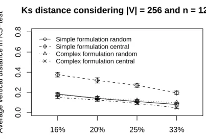
Figures9and10show the error evaluation when we vary the number of nodes and keep|V_|_{= 256}_.

Similar to previous scenario, the results (Figure9) show that in all cases we haveΥ_≤_40%_. Ψ_random_{, in}

both formulation, has a smallerΥ_{-error, because the random choice improves data dispersion. However,}

the simplified formulation has a smallerΥ_{-error. In Figure}₁₀_{, we always have}Φ_≈_5%_{. Again,}Ψ_central_,

in both formulation, has a smallerΦ_{-error because the central elements choice improves the average test.}

Although, the simplified formulation has a smaller Φ_{-error with}₁₂₈_, ₂₅₆ _and₅₁₂ _{nodes, the complex}

formulation presents a better performance for1024nodes.

Figure 9. Υ_{-error considering the delay caused by relay nodes without concurrent traffic.}

Ks distance considering |V| = 256

Number of nodes

128 256 512 1024

0.0

0.2

0.4

0.6

0.8

Figure 10. Φ_{-error considering the delay caused by relay nodes without concurrent traffic.}

Data error considering |V| = 256

Number of nodes

Average error

128 256 512 1024

0.00

0.05

0.10

0.15

Error evaluations suggest that the simplified formulation is more appropriate for small networks and the complex formulation is more scalable. In general, Ψ_random _{is preferable when the}_Rdst _{has higher}

(17)

more appropriate when we have large scale networks. The partial conclusion, considering more realistic real-time scenarios, is that the complex formulation is more appropriate, because the deadlines are met in all cases and the data representativeness is kept.

6.3. Half of Deadlines with Concurrent Traffic

This scenario considers 50%of minimum deadlines (da = dmin/2) with concurrent traffic. We use a 128-node network (we do not consider more nodes due to NS limitations), and vary the percentage of nodes generating data traffic (16%,20%, 25%, and33%of128 nodes) and|V_|₍₂₅₆_, ₅₁₂_, ₁₀₂₄_{, and}

2048). The objective of this scenario is to identify the best strategy in critical applications when the network traffic gradually increases.

In Figure11,dais met only by complex formulation. The reason is that theΨ_{-reduction, in complex}

formulation, is gradually performed during the data routing, and fewer data is delivered. Particularly, when the percentage of nodes generating data is 33%, nearly6.5%of data is delivered by the complex formulation, while 10% is delivered by the simplified formulation. Thus, considering the deadline achievement, the complex formulation is more appropriate in this scenario.

Figure 11. Delay considering the half of deadlines with concurrent traffic.

Delay considering |V| = 2048 and n = 128

Percentage of nodes generating data

Packet delay (s)

16% 20% 25% 33%

2.0

3.0

4.0

5.0

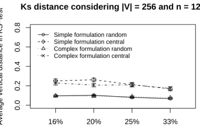
Figures12and13show the error evaluation considering a128-node network, varying the percentage of nodes that generate data traffic, and keeping |V_| _{= 256}_{. As we can see in Figure} ₁₂_{, results show}

that in all cases we have Υ_≤ _30%_{. In both formulations,}Ψ_random _{has a smaller}Υ_{-error. However, in}

the complex formulation,Ψ_central_{presents a smaller}Υ_{-error when we have fewer data traffic (}_16%_and

20%). The reason is that the complex formulation executes fewer consecutiveΨ_{-reductions. Figure}₁₃

shows that, in all cases, we have Φ _≈ _20%_{, note the increase in} Φ_{-error, compared to previous}

scenarios (Φ _≈ _5%_{). The reason is that in both formulations there more consecutive} Ψ_-reductions

affecting data quality. Therefore, considering the confidence interval, both Ψ_{-reductions have the same}

(18)

Figure 12. Υ_{-error considering the half of deadlines with concurrent traffic.}

Ks distance considering |V| = 256 and n = 128

16% 20% 25% 33%

0.0

0.2

0.4

0.6

0.8

Figure 13. Φ_{-error considering the half of deadlines with concurrent traffic.}

Data error considering |V| = 256 and n = 128

Average error

16% 20% 25% 33%

0.10

0.20

0.30

The data error evaluation suggests that the simplified formulation is slightly better than the complex one. However, the partial conclusion, considering this critical and realistic real-time scenario, is that the complex formulation is more appropriate, because deadlines are met and data representativeness is kept. Considering the sampling algorithms, the behavior is kept in bothΨ_{-reduction strategies.}

6.4. Delay Caused by Relay Nodes with Concurrent Traffic

(19)

objective of this scenario is to identify the best strategy when the relay nodes have extra tasks with high priority and the network has a traffic that gradually increases.

Figure14shows the delay results in a128-node network varying the percentage of nodes generating traffic and|V_| _{= 2048}_{. The}_da_{is met in most cases. The complex formulation presents a more scalable}

behavior considering the percentage of nodes generating data. This occurs because the Ψ_-reduction

estimation [Equation7] is related toda,i.e., ifda ≥ dmin theΨ_{-reduction cannot be efficient, when we}

consider other delay aspects, like concurrent traffic.

Figure 14. Delay considering the delay caused by relay nodes with concurrent traffic.

Delay considering |V| = 2048 and n = 128

Packet delay (s)

16% 20% 25% 33%

3

4

5

6

7

8

9

Figure 15. Υ_{-error considering the delay caused by relay nodes with concurrent traffic.}

Ks distance considering |V| = 256 and n = 128

16% 20% 25% 33%

0.0

0.2

0.4

0.6

0.8

Figures 15 and 16 show the error evaluations considering a network with 128-nodes, varying the percentage of nodes generating traffic and|V_|_{= 256}_{. Simplified and complex formulation are presented}

(20)

complex formulation, has a smaller Υ_{-error. The reason is that the complex formulation performs the}

maximumΨ_{-reduction sooner (}Ψ_central_{is executed once or twice). This result shows that because fewer}

successive Ψ_{-reductions are performed, more representativeness is kept in the reduced data,} _i.e._{, data}

degradation is mitigated.

Figure 16. Φ_{-error considering the delay caused by relay nodes with concurrent traffic.}

Data error considering |V| = 256 and n = 128

Average error

16% 20% 25% 33%

0.0

0.2

0.4

0.6

Figure16shows that, in general, we haveΦ_≤_30%_{. The complex formulation with}Ψ_central_presents Φ _≈ _5%_{. The reason is that the} Ψ_central _{has a smaller} Φ_{-error because the central elements choice}

improves the average test and the complex formulation performs the maximumΨ_{-reduction early.}

The errors evaluation suggest that the complex formulation is more appropriate with the Ψ_central

strategy. The partial conclusion, considering this scenario, is that the complex formulation is actually more appropriate, because the deadlines are met in all cases while keeping data representativeness. Considering the sampling algorithm, theΨ_central_{strategy with complex formulation is always indicated.}

7. Conclusions

In real-time applications of wireless sensor networks, the time used to deliver sensor-streams from source to sink nodes is a major concern. The amount of data in transit through these constrained networks has a great impact on the delay. In this work, we presented a data-centric strategy to meet deadlines in soft real-time applications for wireless sensor networks. This work represents shows how to deal with time constraints at lower network levels in a data-centric way.

(21)

As future work, we intend to match the proposed application-level solution with lower-level ones, for example, by considering some real-time-enabled signal processing method. In this case, not only data from a source is reduced, but similar data from different sources is also reduced, resulting in a more efficient solution. Another future work is to use feedback information to enable the source nodes to perform the reduction sooner. However, we intend to improve the central sampling algorithm complexity toO(n), by considering some rank selection algorithms.

Acknowledges

This work is partially supported by the Brazilian National Council for Scientific and Technological Development (CNPq) under the grant numbers 477292/2008-9 and 474194/2007-8.

References

1. Akyildiz, I.F.; Su, W.; Sankarasubramaniam, Y.; Cayirci, E. A Survey on Sensor Networks. IEEE Commun. Mag. 2002,40, 102–114.

2. Lins, A.; Nakamura, E.F.; Loureiro, A.A.F.; Coelho Jr., C.J.N. BeanWatcher: A Tool to Generate Multimedia Monitoring Applications for Wireless Sensor Networks; Marshall, A., Agoulmine, N., Eds.; Springer: Belfast, UK, 2003; pp. 128–141.

3. Nakamura, E.F.; Loureiro, A.A.F.; Frery, A.C. Information Fusion for Wireless Sensor Networks: Methods, Models, and Classifications. ACM Comput. Surv.2007,39, 9/1–9/55.

4. He, T.; Stankovic, J.A.; Lu, C.; Abdelzaher, T. SPEED: A Stateless Protocol for Real-Time Communication in Sensor Networks; IEEE Computer Society: Providence, RI, USA, 2003; pp. 46–55.

5. Li, H.; Shenoy, P.J.; Ramamritham, K. Scheduling Communication in Real-Time Sensor Applications; IEEE Computer Society: Toronto, Canada, 2004; pp. 10–18.

6. Lu, C.; Blum, B.M.; Abdelzaher, T.F.; Stankovic, J.A.; He, T. RAP: A Real-Time Communication Architecture for Large-Scale Wireless Sensor Networks; IEEE Computer Society: San Jose, CA, USA, 2002; pp. 55–66.

7. Aquino, A.L.L.; Figueiredo, C.M.S.; Nakamura, E.F.; Loureiro, A.A.F.; Fernandes, A.O.; Junior, C.N.C. On The Use Data Reduction Algorithms for Real-Time Wireless Sensor Networks; IEEE Computer Society: Aveiro, Potugal, 2007; pp. 583–588.

8. Li, P.; Gu, Y.; Zhao, B.A Global-Energy-Balancing Real-time Routing in Wireless Sensor Networks; IEEE Computer Society: Tsukuba, Japan, 2007; pp. 89–93.

9. Pan, L.; Liu, R.; Peng, S.; Yang, S.X.; Gregori, S. Real-time Monitoring System for Odours around Livestock Farms; IEEE Computer Society: London, UK, 2007; pp. 883–888.

10. Peng, H.; Xi, Z.; Ying, L.; Xun, C.; Chuanshan, G. An Adaptive Real-Time Routing Scheme for Wireless Sensor Networks; IEEE Computer Society: Niagara Falls, Ontario, Canada, 2007; pp. 918–922.

(22)

12. Altiparmak, F.; Tuncel, E.; Ferhatosmanoglu, H. Incremental Maintenance of Online Summaries over Multiple Streams. IEEE Trans. Knowl. Data Eng. 2008,20, 216–229.

13. Datar, M.; Gionis, A.; Indyk, P.; Motwani, R. Maintaining Stream Statistics over Sliding Windows.

SIAM J. Comput. 2002,31, 1794–1813.

14. Guha, S.; Meyerson, A.; Mishra, N.; Motwani, R.; O’Callaghan, L. Clustering Data Streams: Theory and Practice. IEEE Trans. Knowl. Data Eng. 2003,15, 515–528.

15. Lian, X.; Chen, L. Efficient Similarity Search over Future Stream Time Series. IEEE Trans. Knowl. Data Eng. 2008,20, 40–54.

16. Akcan, H.; Bronnimann, H. A New Deterministic Data Aggregation Method for Wireless Sensor networks. Signal Process.2007,87, 2965–2977.

17. Bar-Yosseff, Z.; Kumar, R.; Sivakumar, D. Reductions in Streaming Algorithms, with an Application to Counting Triangles in Graphs; ACM: San Francisco, CA, USA, 2002; pp. 623–632. 18. Buriol, L.S.; Leonardi, S.; Frahling, G.; Sholer, C.; Marchetti-Spaccamela, A. Counting Triangles

in Data Streams; ACM: Chicago, IL, USA, 2006; pp. 253–262.

19. Cammert, M.; Kramer, J.; Seeger, B.; Vaupel, S. A Cost-Based Approach to Adaptive Resource Management in Data Stream Systems. IEEE Trans. Knowl. Data Eng. 2008,20, 202–215.

20. Indyk, P. A Small Approximately min–wise Independent Family of Hash Functions; ACM: Baltimore, MD, USA, 1999; pp. 454–456.

21. Abadi, D.J.; Lindner, W.; Madden, S.; Schuler, J. An Integration Framework for Sensor Networks and Data Stream Management Systems; Morgan Kaufmann: Toronto, Canada, 2004; pp. 1361–1364.

22. Babcock, B.; Babu, S.; Datar, M.; Motwani, R.; Widom, J. Models and Issues in Data Stream Systems; ACM: Madison, WI, USA, 2002; pp. 1–16.

23. Gehrke, J.; Madden, S. Query processing in Sensor Networks. IEEE Pervasive Comput. 2004,

3, 46–55.

24. Madden, S.R.; Franklin, M.J.; Hellerstein, J.M.; Hong, W. TinyDB: An Acquisitional Query Processing System for Sensor Networks. ACM Trans. Database Syst. 2005,30, 122–173.

25. Xu, J.; Tang, X.; Lee, W.C. A New Storage Scheme for Approximate Location Queries in Object-Tracking Sensor Networks. IEEE Trans. Parallel Distrib. Syst.2008,19, 262–275.

26. Elson, J.E. Time Synchronization in Wireless Sensor Networks. PhD. Thesis, University of California, Los Angeles, CA, USA, 2003.

27. Yu, Y.; Krishnamachari, B.; Prasanna, V.K. Data Gathering with Tunable Compression in Sensor Networks. IEEE Trans. Parallel Distrib. Syst. 2008,19, 276–287.

28. Yuen, K.; Liang, B.; Li, B. A Distributed Framework for Correlated Data Gathering in Sensor Networks. IEEE Trans. Veh. Technol. 2008,57, 578–593.

29. Zheng, R.; Barton, R. Toward Optimal Data Aggregation in Random Wireless Sensor Networks; IEEE Computer Society: Anchorage , AK, USA, 2007; pp. 249–257.

30. Chen, M.; Know, T.; Choi, Y. Energy-efficient Differentiated Directed Diffusion (EDDD) in Wireless Sensor Networks. Comput. Commun.2006,29, 231–245.

(23)

32. Gedik, B.; Liu, L.; Yu, P.S. ASAP: An Adaptive Sampling Approach to Data Collection in Sensor Networks. IEEE Trans. Parallel Distrib. Syst. 2007,18, 1766–1783.

33. Matousek, J. Derandomization in Computational Geometry. Algorithms1996,20, 545–580. 34. Bagchi, A.; Chaudhary, A.; Eppstein, D.; Goodrich, M.T. Deterministic Sampling and Range

Counting in Geometric Data Streams. ACM Trans. Algorithms2007,3, Article number 16.

35. Nath, S.; Gibbons, P.B.; Seshan, S.; Anderson, Z.R. Synopsis Diffusion for Robust Aggregation in Sensor Networks. InProceedings of 2nd International Conference on Embedded Networked Sensor Systems, Baltimore, MD, USA, 2004; pp. 250–262.

36. Aquino, A.L.L.; Figueiredo, C.M.S.; Nakamura, E.F.; Buriol, L.S.; Loureiro, A.A.F.; Fernandes, A.O.; Junior, C.N.C. A Sampling Data Stream Algorithm For Wireless Sensor Networks; IEEE Computer Society: Glasgow, Scotland, 2007; pp. 3207–3212.

37. Aquino, A.L.L.; Figueiredo, C.M.S.; Nakamura, E.F.; Frery, A.C.; Loureiro, A.A.F.; Fernandes, A.O. Sensor Stream Reduction for Clustered Wireless Sensor Networks; ACM: Fortaleza, Brazil, 2008; pp. 2052–2056.

38. Nakamura, E.F.; Figueiredo, C.M.S.; Nakamura, F.G.; Loureiro, A.A.F. Diffuse: A Topology Building Engine for Wireless Sensor Networks. Sign. Proces. 2007,87, 2991–3009.

39. Reschenhofer, E. Generalization of the Kolmogorov-Smirnov test. Comput. Stat. Data Anal.1997,

24, 422–441.

40. Aquino, A.L.L.; Loureiro, A.A.F.; Fernandes, A.O.; Mini, R.A.F. An In-Network Reduction Algorithm for Real-Time Wireless Sensor Networks Applications; ACM: Vancouver, British Columbia, Canada, 2008; pp. 18–25.

41. Bustos, O.H.; Frery, A.C. Reporting Monte Carlo results in statistics: suggestions and an example.

Rev. Soc. Chi. Estad.1992,9, 46–95. c