i
UBONG SYLVANUS UDOETTE
Dissertation report presented as partial requirements for
obtaining the Master’s degree in Statistics and Information
Management
Imputation Techniques for Improving Survey Outcomes
in Nigeria: The Case of the Business Expectation Survey
ii
Title:
Imputation Techniques for Improving Survey
Outcomes in Nigeria: The Case of the Business
Expectation Survey (BES) of the Central Bank of
Student full name :
UBONG SYLVANUS UDOETTE
full name
2016
2016
Title:
Imputation Techniques for Improving Survey
Outcomes in Nigeria: The Case of the Business
Expectation Survey (BES) of the Central Bank of
Nigeria
Student full name :
i
NOVA Information Management School
Instituto Superior de Estatística e Gestão de Informação
Universidade Nova de Lisboa
Imputation Techniques for Improving Survey Outcomes in Nigeria: The
Case of the Business Expectation Survey (BES) of the Central Bank of
Nigeria
by
Ubong Sylvanus Udoette
Proposal of
dissertation presented as partial requirement for obtaining the Master’s degree
in Statistics and Information Management, with a specialization in Analysis and Information
Management
Advisor:
PROFESSOR DOUTOR PAULO JORGE GOMES
ii
DEDICATION
I dedicate this project to GOD Almighty who made it possible financially and otherwise as
well as to my parent Mr & Mrs Sylvanus B. Udoette who laid the foundation for my
education.
I am also grateful to my wife, Mrs Unyime U. Udoette and my children (Caleb, Covenant,
iii
ACKNOWLEDGEMENTS
My sincere appreciation goes to Dr. Sanni I. Doguwa, former Director of Statistics, Central
Bank of Nigeria (CBN), for the information about the school and programme. Special thanks
goes to Dr. Olowofeso Olorunsola, a Deputy Director in the Statistics Department, CBN for
accepting the additional responsibity of being our resident supervisor/examiner, which
required having to sometimes spend several hours after official working hours to supervise
our examinations and other programme requirements.
Special thanks goes to Dr Joa, Director of Statistics, Bank of Portugal (BP) and his entire team
for their support during the programme and our study visit to BP. Not forgetting my
colleagues at the CBN such as Mr B. S. Omotosho, Dr. Bamanga, Mr. Manya and Dr. Kufre
Bassey for their help in making this a reality as well as the institution (CBN) for the
iv
ABSTRACT
Over the years, the issue of respondents’ apathy, missing data and item non
-response in
particular, has remained a major concern with regards to analyses of survey-based studies
undertaken by the Central Bank of Nigeria (CBN). Researchers and policy analysis within the
CBN has been plagued by the growing quantum of item non-response. This dissertation will
attempt to empirically analyze and recommend the best imputation technique for item
non-response in surveys undertaken by the Bank. The case in point will be the Business
Expectations Survey (BES) conducted quarterly by the CBN. It will take a specific
items/questions in the BES for which there are complete responses and undertake a multiple
correspondence analysis (MCA) of the responses. Using a complete randomize scheme (table
of random numbers) it will exclude 15
–
35 percent of responses as if they were item
non-response and proceed to replace them through various imputation technique. After which the
MCA will be repeated for each of the derived data sets and the result compared with that of
the original data sets. The matrices of principal coordinates
are compared using the RV
coefficient (Escoufier, 1973), a measure of similarity between two datasets such that a value
of 1 indicates complete similarity and 0 indicates complete dissimilarity. This coefficient is a
generalization of the square of S
pearman’s correlation coefficient
. The result of the RV
coefficient analysis and well as the analysis of some selected summary statistics will be used
to recommend the best imputation technique for such item non-responses in future surveys.
KEYWORDS
Missing Data; Item Non-response; Imputation Technique; RV Coefficient; Multiple
v
INDEX
1.
Introduction ... 1
2.
Literature review ... 3
2.1.
THEORETICAL FRAMEWORK ... 3
2.1.1.
MISSING DATA IMPUTATION TECHNIQUES ... 9
2.2.
EMPIRICAL REVIEW OF LITERATURE ... 14
3.
Methodology ... 17
4.
Results and discussion ... 22
5.
Conclusions ... 25
6.
Limitations and recommendations for future works ... 26
7.
Bibliography ... 28
8.
Appendix (ANALYTICAL TABLES) ... 31
vi
LIST OF FIGURES
vii
LIST OF TABLES
viii
LIST OF ABBREVIATIONS AND ACRONYMS
BES
Business Expectation Survey
CBN
Central Bank of Nigeria
IQR
Inter-quartile Range
NBS
National Bureau of Statistics
NIPALS
Non-linear Iterative Partial Least Squares
MAR
Missing at Random
MCA
Multiple Correspondence Analysis
MCAR
Missing Completely at Random
MI
Multiple Imputation
MNAR
Missing not at Random
1
1.
INTRODUCTION
In any empirical research it is almost impossible to avoid the problem of missing data.
Determining the best and most appropriate imputation technique in handling missing data
during analyses plays a vital role in sufficiently reducing the statistical bias in such studies
and ensuring that valid conclusions are made about the target population. In practice,
however, the first option available to most researchers in handling missing data is deleting
cases with missing values (trimming or winsoring), especially when the missing data does not
occur in more than 5 per cent of the entire cases. This option, usually result in a reduction in
the sample size which has significant adverse effect on the statistical power of the derived
estimates. The impact on statistical estimates is also believed to be more pronounced in
cases where the missing values are systematically or completely different from the cases
where complete information are available Langkamp et al (2011).
The problem of missing data is more pervasive with regards to research/studies that require
sample surveys. Some respondents may not be willing to participate in a survey (unit
non-response) altogether or they are unwilling to provide answers to some specific questions
that are required (item non-response). Missing data may also arise from transcription errors
or when certain sampling units are dropped in follow-up surveys or when trying to merge
two data sets that do not match Brand, J.P (1999). However, there are several modern
alternatives to missing data analyses other than complete case-wise deletion. These ranges
from imputation with plausible value by researchers using simple techniques such as the
mean of the observed cases for each variable to more complicated models such as
regression imputation, stochastic regression imputation, maximum likelihood, multiple
imputation, etc. Moreover, case-wise deletion may in some cases lead to significant
reduction in available data; data wastage of more than 20 per cent is quite common.
The Statistics Department, CBN conducts a quarterly Business Expectations Survey (BES) of
leading firms drawn from various sectors across the Nigerian economy. The sampling frame
for the survey is an aggregation of the establishment survey business registers of the CBN
and the National Bureau of Statistics (NBS). Respondents are drawn from the Industrial,
2
Financial Intermediation, Hotels and Restaurants, Renting & Business Activities and
Community & Social Services. The BES result provides advance indication of change in the
overall business activity in the economy and in the various measures of activity of the
companies’ own operations as well as selected economic indicators.
Recent BES have
produced an average response rate of 95 - 98.5 per cent; indicating increasing respondent
apathy. Item non-response has also been on the increase among survey respondents and
has become a major concern in the analyses of the survey returns.
Usually, the immediate options available to data analysts of the BES have been case-wise
deletion of cases with item non-response or a discretionary choice of any of the available
imputation technique to address such cases. However, with the increasing size and quantum
of the item non-response and the likely effect each adopted imputation technique may have
on the survey outcome, it is becoming increasing necessary for the Department/CBN to have
a standardized way of addressing this problem and not leave it at the discretion of individual
analyst. This dissertation is geared towards addressing these issues and thus be in a position
to recommend to the CBN the best imputation technique to be adopted in handling cases of
item non-responses in future survey analyses.
The specific objectives of this research include the following:
To review the various imputation techniques used by data analyst for
addressing missing data issues in the analysis of the BES of the CBN
Assess the statistical biases introduced by the various imputation techniques in
the data set
3
2.
LITERATURE REVIEW
2.1.
THEORETICAL
FRAMEWORK
Missing data refers to a condition where some part of the required information about a
particular phenomenon of interest is missing or not available. This entails that values are not
available for the variable of interest for some observations. In empirical research, there are
three major reasons why data might be missing, namely: study design, characteristics/type
of respondents and the interaction between respondents and the survey design. Missing
data occur mainly as a result of non-response which could be as a result of a number of
other factors such as non-availability of information for one or more subject; non-response
to sensitive questions; the amount of time required to complete questionnaire by
respondents; cases where participants drop out before the test ends and measurements are
taken, etc. These missing observations
greatly inhibit the researchers’ ability
to understand
the nature of the phenomena and the extent of this inhibition is not often known.
Theoretically, there is also a
n important distinction between “unit missing data” commonly
referred to as unit non-
response and “missing values” or what is called item non
-response.
Unit missing data occurs when the data for a particular respondent/unit of analysis is not
available. In practice this occurs when some respondents or unit of the target population
refuses to partake in selected surveys or drop out. The second case, which is missing values,
refers to the situation where the scores for particular variables are missing for some
sampling units thus its common name “item non
-
response”.
There are three major areas in the discussion about the impact of missing data. These are
measurement; understanding the relationship between variables; and drawing conclusion
based on the available information. However, the main concern about missing data is the
common threat it possess to the validity of the conclusions drawn in most research work
irrespective of the field or sphere of research. However, there are two other main issues that
must be taken into account when dealing with missing data. The first is the issue of the
amount of the missing data in a particular data set. Generally, the size of the missing data is
presumed to be directly proportional to the impact such missing data will have on the
statistical inference about the data set; the higher the missing data, the higher its impact on
4
parameters that would be generated from the incomplete data set. The second major
concern about missing data is usually about the actual process that causes the missing data,
which is believed to have significant impact on the validity of the study findings. Missing data
can affect both the reliability (stability, consistency, or reproducibility) and validity (accuracy,
verisimilitude, or ability to generalize) of research findings.
In order to facilitate it diagnoses and identify the proper remedy to handling missing data,
statistician developed a classification system for missing data. The various types of missing
data are associated with different consequences that influence action to remedy the
problem. And sometimes the diagnosis indicates that there is no remedy available. In
longitudinal studies, there are situations where data are missing at a particular occasion of
measurement, a phenomena commonly referred to as
“missing wave”
. In multilevel studies
in which participants are grouped into larger sampling units,
“unit missing data” can occur
at the individual /participants level or at the group level (hospitals, schools, banks). Data can
also be missing cross-sectional (for sampling units observed at a single occasion) or across
time in longitudinal studies.
To be able to decide how to handle missing data, it is important to try to understand why
the data was missing in the first instance or what is commonly referred to as
“missingness
mechanisms”
. These are basically assumptions about the occurrence of the missing data
based on a hypothetical perception of the existence of a complete data set. Thus the missing
data are viewed as data entries which were not observed or measured, but could have been.
There are three (3) basic
“
missingness
”
assumptions or classifications, namely:
Missing completely at random (MCAR):
The missing data for a variable is said to
follow a MCAR process if the probability of missingness is the same for all units. That
is, the probability that an observation Xi is missing is unrelated to the value of Xi or
the value of any other variables. In other words, a missing data mechanism is called
MCAR, if the probability of each entry missing is independent of the values in the
hypothetical complete data set. The assumption here is that for each variable with
missing data, the observed values constitute a random sub-sample of the original
complete data set of the variable. It is generally believed that if a set of missing data
5
whatever inferences is made from the remaining data set. Bennet, D. A (2001)
further noted that valid inferences could be drawn from the analysis of a data set
with missing data following a MCAR process using any of the analysis technique.
Missing at random (MAR)
: In most cases, the missing data are not completely at
random; they are either related to the missing values themselves or other observed
values. A set of missing data is said to be a MAR if the propensity for a data point to
be missing is not related to the missing data but to some of the observed data. In
other words, If the probability of an observation to be missing depends on previously
observed data and not on the variable that contain the missing data, then the
underlying missing data mechanism is called a MAR. The basic concept of a MAR
suggests the existence of a minimal criterion upon which valid statistical analysis can
be undertaken with the data set without modelling the underlying missing data
mechanism. In a MAR, the observed data has all the information required to
undertake a valid statistical analysis of the missing data. However, the information
may be structured in a way that makes the analysis complicated. It is therefore
becomes imperative that all observed data be taken into account in order to
undertake any valid statistical analysis. The condition in which the missing data is a
MAR is most often referred to as
“
ignorable missingness
”
–
this name comes from
the fact that the available data we can still generate unbiased parameter estimates
without necessarily needing to provide a model to explain the pattern of missingness.
For example, the different nonresponse rates for two major groupings of
respondents say “whites“ and “blacks” indicate that a particular
question say
“earnings” in the Social Indicators Survey is not missing completely at random. A
more general assumption, missing at random, is that the probability a variable is
missing depends only on available information. Thus, if sex, race, education, and age
are recorded for all the people in the survey, then “earnings” is missing at random if
the probability of non-response to this question depends only on these other, fully
recorded variables. Thus, any model for earnings would have to include variable
predictors for race, to avoid non-response bias.
Missing not at random (MNAR):
If a set of missing data do not follow a MCAR or
6
Rubin, D. B (1987), a missing data mechanism will be a MNAR if the missing values
depend on the variable itself. For example, if in a survey people with low income are
less likely to report their income, then the missing data are not at random (MNAR)
because the non-response is simply because of the question being asked. In such
case the only way to obtain an unbiased estimate of parameter is to model the
missingness. This entails the need to write a model that accounts for the missing
data. Gelman, A and Hill, J (2006) identified two categories of MNAR process, namely:
i.
Missingness that depends on unobserved predictors
: Missingness is no longer
“at random” if it depends on information that has not been recorded and this
information also predicts the missing values. For example, suppose that
people with college degrees are less likely to reveal their earnings, having a
college degree is predictive of earnings. Thus earnings are not missing at
random.
ii.
Missingness that depends on the missing value itself
: Finally, a particularly
difficult situation arises when the probability of missingness depends on the
potentially missing variable itself. For example, suppose that people with very
higher income are less likely to reveal them. Thus the missing data are only
information of very high earners (observations with the highest group of
values for the variable will then be missing). This become even more difficult
to model
.
The first step in addressing the problem of missing data is being able to identify the
underlying missing data mechanisms. A Proper diagnostic of the missing data mechanism
informs the researcher about the likely inferential limitations in using the observed data set
and the need for caution, if need be, when interpreting the results. A number of researches
have been undertaken in this area of missing data diagnostics. Nakagawa, S and Freckleton,
R.P (2010) stated that being able to correctly identify the missing data mechanism would
enable the researcher to make a decision on the most appropriate technique to address the
issue. The authors identified some visual inspection technique to be used in determine
whether the missing data is a MCAR or not. They noted however, the difficulty in using this
simple visual inspection technique in distinguishing between a MAR and MNAR. Little, R. J
7
while Schafer, J. L (1997) concluded that distinguishing between MAR and MNAR would
require additional information regarding the distribution of the missing data.
It is equally important for researchers to assess the extent of missing data before using such
information in any analysis. There are several methods/procedures identified in literature
for assessing the extent of missing data. This includes:
List-wise or complete case method
: A simple way of assessing the extent of missing
data is to examine the number of cases with missing data for at least one variable. A
lot of statistical software packages which are designed to handle inferential statistical
procedures have List-wise deletion as the default for handling missing data. These
packages generate and report the amount of missing data as the number of cases
with missing data for at least one variable.
Complete variable method
: this method provides an estimate of extent of the missing
data by looking at the proportion of variables than contain missing values.
Available
Case method
: The extent/amount of missing data can also be defined in
terms of the number of missing values for each variable (a method sometimes
referred to as pair-wise deletion). The available case method is considered
complementary method to the complete case approach in diagnosing the amount of
missing data.
Sparse matrix method
: In the sparse method, the extent/amount of missing values is
computed using the total data matrix.
The ratio method
: in the ratio method, the extent of missing data is computed as an
index ri defined by the ratio of the sparse matrix method to the complete case. This
ratio offers an average amount of the missing variables per incomplete case. The
higher the ratio, the more the extent of missing data. An alternative way of
computing ri is as the ratio between the sparse matrix and proportion of incomplete
variables
–
which simply provide the proportion of missing cases per incomplete
variable
A combination of these five diagnostic procedures would provide sufficient information
8
there are five basic steps to follow in selecting the most appropriate solution to handling
missing data. These are:
Identifying the relevant variables:
identifying the specific variables for analysis is
usually considered the first step before reviewing what data set/information may
be missing. This basic approach provides a simplified diagnostic step as well as the
treatment for the missing data.
Specify the level of analysis at which data are missing:
Having identified the
variable of interest, deciding on the level of analysis is an important preliminary
step in the missing data analysis process. When aggregate level is the focus of the
analysis and the aggregates are directly derived from the micro data sets, missing
data at the micro level do not pose significant problem to achieving the set
objectives. However, missing data at macro level can create significant bias if the
analysis performed at micro/unit level.
Conduct missing data techniques
: There are a number of factors to consider
before deciding on the technique to be used in analysis a data set with missing
data. This includes:
i.
If the missing data mechanism is known
:
It is important in missing data
analysis to ascertain if missing data is of “ignorable type” –
MCAR or MAR.
If “ignorability” is ascertained or likely, methods such as imputation and
model/based parameterization methods are preferred. However, if the
missing data are not ignorable
–
MNAR, then the relevant variables needed
to model the missing values are not available.
ii.
The amount of missing data
: The amount of missing data is believed to
have significant impact on the level of precision of the parameter
estimates. However, when the sample size is large and the percentage of
cases of missing data is relatively small (≤1%), data d
eletion may be a
reasonable solution if the missing data are ignorable. If the missing data is
a MCAR, little information is lost even when a certain percentage of the
data is missing. The reverse is true for a MNAR even when a small amount
9
Identifying the Statistical Model and test to be used
: a procedure that uses the
available raw data to estimate the parameters such as liner models do not always
require the complete data. However, procedures that rely on generated values
such as
“covariance matrix” for estimation of the parameters generally require
complete information/data cases.
Identifying the statistical software to use:
it is important for data analyst to be
familiar with the default procedures for handling missing data for particular
statistical software that are to be employed for analysis. Awareness of default
methods is important for the evaluation of appropriateness of a particular missing
data conditions
2.1.1.
MISSING DATA IMPUTATION TECHNIQUES
Having identified the extent of missing data, the missing data pattern/mechanism and
undertaken the diagnostics procedures highlighted above, it is imperative to now discuss the
various concepts or approaches to handling missing data. Several techniques are identified
in literature to addressing the issue of missing data. These include:
2.1.1.1.
CONVENTIONAL METHODS
Case-wise Deletion:
Case-wise deletion
is the most common method identified in
literature for handling missing data
. It is also referred to as the “
complete-case
analysis
” or “lis
t-
wise deletion”
(Gelman, A. & Hill, J (2006) and Knol, M, J
et al
.
(2010)) and implemented as the default procedure in most software packages. This
technique involve discarding all observations with at least one missing value resulting
in a reduction in number of observations in the data set that is available for analysis.
Little, R. J and Rubin, D.B (2002) noted that the major limitation/concern to the use
of the case-wise deletion is the possible loss of information associated with this
technique which may lead to concerns about the statistical power of the analysis
thereof. Studies such as Klebanoff, M. A & Cole, S. R (2008) and Nakai, M & Weiming,
K. (
2011)
has shown that if missing data mechanism are not MCAR, case-wise deletion
are likely to generate biased parameter estimates which may lead to incorrect
10
Available Case Analysis:
Another conventional technique to addressing the problem
of missing data is the available case analysis. The available case analysis refers to a
group of techniques that uses the available data to estimate the means and
covariance. One of the popular methods in this group is called pair-wise deletion.
This method focuses on the variance-covariance matrix (or correlation), which is
computed based on the observations with complete data for each pair of variables.
Single imputation
: This is a simple and very common approach to handling missing
data. It involves filling or “imputing” some form of
single value estimated for the
missing value and undertaking analysis with the data derived as if there were not
missing in the first place. There are a number of single imputation procedures in
literature, namely:
I.
Replacement with a constant
a)
Mean Replacement
: Is a common procedure adopted in social
sciences in treating missing data. It is easily implemented by most
statistical packages. It involves replacing each missing value with the
sample mean of the observed values for the particular variable. The
major disadvantage of this technique is that it distorts the original
distribution of the variable and relationship with other variables.
Gelman, A. & Hill, J (2006) noted its “pulling” ability in terms of
tending the correlation between variables towards zero. Imputing
mean values severely under-represents extreme values which lead to
a decrease in variance. Soley-Bori, M (2013) identified this procedure
as the “marginal mean imputation” and provide a distinction with
what is called “conditional mean imputation” which is considered a
non-random imputation technique.
b)
Median imputation
: This is just a slight variance of the mean
imputation. As noted earlier, mean imputation has significant impact
on extreme values. This impact becomes even more sever when the
underlying distribution is skewed, very flat or peaked. In this case, the
11
better model of the underlying distribution hence the concept of
median imputation.
c)
Zero imputation
: This commonly implemented for binary response
variables. In such studies, incomplete response maybe considered
incorrect or false and in such circumstances zero imputation are
justified. However, serious consideration should be given to the
meaning of the value 0 with relation to the variable of interest before
adopting zero imputation.
d)
Last value carried forward
: this is a very conservative approach that is
commonly adopted in health/medical related research. It involves
carrying forward the last recorded value of the variable to fill the next
missing value. Gelman, A. & Hill, J (2006) noted however, that the last
value carried forward method of imputation introduces significant bias
in the analysis outcome in missing data analysis.
II.
Replacement with a randomly selected value:
There are two basic
approaches in random imputation methods for missing data. These are:
a)
Empirical procedures
: This involves using the available data to
randomly estimates and replaces the missing values. Example of this
procedure include:
Hot-deck imputation
: This is a nonparametric technique that
does not require making any underlying assumption about the
distribution of the variable with missing values. It involves
randomly selecting a value from the observed data to replace a
missing value.
The missing values in the variables of interest
are estimated using other similar observed values with the
probability of selecting one observed value over another
dependent on the rate at which the different values occur.
Another simple hot-deck imputation procedure is replacement
with values from the
nearest neighbor
. Generally, hot-deck
imputation is believed to have significant effect on standard
12
Cold-deck imputation
: this an imputation technique in which
values from other data set are used to replace the missing
values in the current data set. It is commonly used in related
survey based researches where responses from same/similar
respondents are used to replace non-response in current
surveys.
b)
Model-based procedures
: This involves using models to generate
estimates given the observed data sets, the relationship amongst the
variables and other constraints imposed by the underlying
distribution. According to Piggot, T. D (2001), model-based procedures
requires the researcher to make assumptions about the joint
distribution of all the variables and the nature of the missing data. The
underlying distribution can be a Bernoulli or binomial distribution (for
outcomes with two distinct possibilities only), a poisson distribution
(for counted variables) or a multinomial distribution (for unordered
categorical variables).
III.
Replacement with a non-randomly derived value:
An example of the
non-random simple imputation technique is the
Conditional Mean
procedure.
Here, the missing values are replaced with means of the classification
variables. The mean that are used in place of the missing values for each
variable are not computed using the entire sample, they are means of
strongly related classification variable within the different groups.
Overall, single imputation techniques are believed to underestimate standard errors
thereby increasing the likelihood of rejecting a true null hypothesis (committing a
type I error). These procedures also introduce a lot of other biases and tend to
perform poorly even when the missing data follows a MAR or MCAR process.
However, procedures such as mean imputation, zero imputation and last value
carried forward are the easiest technique in handling missing data.
Multiple imputation:
In practice, having missing data in a number of variables of
interest in the available data set is a common occurrence in which case applying any
13
set becomes a multivariate outcome in which any of the components can be missing.
Rubin, B.D (1987) noted that multiple imputation (MI) is a technique of replacing all
the missing values/observation in a data set by a vector of plausible values. The
author highlighted the advantages of MI to include: better statistical validity; higher
statistically efficiency; adaptability to modern and sophisticated statistical software.
The use of a vector of plausible value and not just a single imputed value also
addresses the concerns of accuracy, variance and standard error raised in the
discussion of single imputation. However, Soley-
Bori, M (2013) highlighted that “MI
solves the limitations of single imputation by introducing an additional form of error
based on variation in the parameter estimates across the imputation, which is called
between imputation error
”. And that “
When the data is MAR, multiple imputation
can lead to consistent, asymptotically efficient, and asymptotically normal
estimates”. Alliso
n, P. D (2000) reiterated the basic steps in MI as proposed by Robin,
B. D (1987) as:
i.
Impute missing values using an appropriate model that incorporates random
variation.
ii.
Do this M times (usually 3-
5 times), producing M “complete” data sets.
iii.
Perform the desired analysis on each data set using standard complete-data
methods.
iv.
Average the values of the parameter estimates across the M samples to
produce a single point estimate.
v.
Calculate the standard errors by :
o
averaging the squared standard errors of the M estimates
o
calculating the variance of the M parameter estimates across
samples, and
o
combining the two quantities
2.1.1.2.
ADVANCED METHODS
Apart from MI, there are a number of other advance imputation techniques in missing data
analysis. Most of these techniques are maximum likelihood and Bayesian procedure which
14
i.
EM Agorithm
: The EM algorithm generates maximum likelihood estimates through a
set of an interactive software procedure. At the E-step, observations are read into
the system one at a time; if data is reported then the sums, sums of cross products
and the sums of squares are augmented. If however, no value is reported, then a
regression based best guest of the value is adopted. The M-step entails the
estimation of the mean, variance and covariance based on the retained values of the
sums, sums of cross products and the sums of squares. Being an interactive
application, the based guest of the missing values is updated during the next E-step
based on the computed covariance and new regression for predicting each variable.
However, the EM algorithm does not generate standard errors but its parameter
estimates are as good as any other maximum likelihood estimator.
ii.
Full Information Maximum Likelihood
: The full information maximum likelihood
(FIML) otherwise known as “Direct Maximum Likelihood” generated unbiased
parameter estimate as well as standard errors for MCAR and MAR. The procedure
entails the estimation of a likelihood function for each observation based on the
available data and variables. FIML procedure uses all the information in the data set.
It generates the mean and variance for the missing observations in each variable by
using the information observed for other variables for those points.
iii.
Non-Linear Iterative Partial Least Squares (NIPALS)
: This category of models was
first developed in the area of Chemistry (chemo-metrics and analytical chemistry)
because of the analytical problem of strong non-linear relationship in data sets. It is
precipitated on the argument that although linear model would provide simple
approximation of non-linear problems, such models perform poorly whenever the
non-linearity issues are very sever. NIPALS modeling was introduced by pioneer
works of Wold, H (1974) and S. Wold, Kettaneh-Wold, N. and Skagerberg (1989). It
involves applying a non-linear transformation of the observed variables,
reconstruction of a new linear representation, and application of the basic principles
of partial least squares.
2.2.
EMPIRICAL
REVIEW
OF
LITERATURE
The problem of analyses with missing data was revolutionized in 1987 with two major
15
Surveys” by Donald B. Rubin and a joint publication by Roderick J. Little and Rubin titled
“Statistical Analysis with Missing Data”. These two significant publications and two other
articles by Allison (1987) and Muthen et al (1987) on structural equation models for analyses
with missing data as well as the growing involvement of personal computers set the tone for
the development of several missing data analyses software in the next two decades.
Subsequent publication by Tanner, M.A and Wong, W.H (1987) on data augmentation would
also set the stage for software applications on analyses on missing data using multiple
imputations. They noted that augmentation scheme makes it possible to easily analysis data
sets with missing values with
the assumption that every data set is augmented by a “latent”
data set.
Over the years, several methods have evolve in handling the problems of missing data (most
of which have discussed in the section above). Piggot, T. D (2001) provided a review of these
methods by using data from an intervention study designed to increase students' ability to
control their asthma symptoms. The paper applied the complete case analysis, available
case, maximum likelihood and multiple imputations on the data set and compared the
results. The author found that although the point estimates provided by available case were
quite close to the model based methods, there were however, no statistically
limits/conditions as to when the estimates from the available case would continue to be
unbiased. Raghunathan, T.E (2004) also reviewed three approaches for analyzing incomplete
data, namely: weighting available responses, multiple imputations and maximum likelihood.
He found the maximum likelihood to be the best method since it works directly with the
likelihood of the observed incomplete data.
Soley-Bori, M (2013) reviewed the key assumption and methods of applied analysis with
missing data. The author reviewed the missing data mechanisms, the patterns of
missingness as well as the conventional methodologies in missing data analysis such as
list-wise deletion, imputation methods, multiple imputation, maximum likelihood and Bayesian
methods; highlighting the advantages and limitations in each case. The paper compared the
various methods of imputation for missing data by simulating with random values set to
missing. The author also provided a practical review of the analysis of missing data in SAS,
16
Yuan, Y. C. (2000) reviewed the basic concepts of missing data, the various methods of
analysis as well as the applications of some multiple imputation procedures. The paper also
introduced a new SAS procedure (introduced with the SAS 8.0) for implementing multiple
imputations for multivariate data set with missing observations as well as the
analysis/interpretation of the results from multiply imputation. Graham, J.W (2009)
presented a summary of literature on missing data with theoretical backgrounds and
descriptions of a number of multiple imputation techniques as well as maximum likelihood
methods. The author also discussed a number of practical issues that researchers face in
missing data analysis in real life. The study concluded that the quality of research have been
enhanced in recent years with availability of several useful computer programs and
applications for analyzing missing data with capabilities of performing procedures such as
multiple imputation with the normal model or maximum likelihood methods.
Reiter, J.P and Raghunathan, T (2007) examined the adaptations of the multiple imputation
framework to missing data cases in large and small samples size, issues of data
confidentiality, and measurement error. They found that the application of the multiple
imputation framework has gone beyond the traditional context of non-response in large
sample survey to Individual researches with relative samples mainly with the development in
17
3.
METHODOLOGY
While most research in this area are geared towards theorectically reviewing the various
imputation techniques, this dissertation would be more practical in undertaking and
quantifying the implication of the various imputation technique on analysis outcome using a
part of the data from the BES of the CBN. The project will undertake a principal component
analysis (PCA) of the responses in the BES by resp
ondents for the question: “How do you
agree on the impact of the following constraints on your business”. The question is basically
tr
ying to capture respondents’ perception on the
various factors that affect their business
and business generally, in Nigeria. The following 12 identified constraints are available to
respondents:
i.
High Interest Rate
ii.
Unclear Economic Law
iii.
Lack of Equipment
iv.
Insufficient Demand
v.
Access to Credit
vi.
Financial Problem
vii.
Competition
viii.
Labour Problems
ix.
Lack of Materials Input
x.
Unfavourable Political Climate
xi.
Unfavourable Economic Climate
xii.
Insufficient Power Supply
Respondents are expected to rate the impact of the 12 factors listed above on business for a
given quarter using 5-point Likert-type scale to show their level of agreement/disagreement:
Strongly Agree
Agree
Neither Agree nor Disagree
Disagreed
Strongly Disagree
During the analysis, these five levels of responses are treated as an interval scale and
18
Strongly Agree
–
5
Agree
–
4
Neither Agree nor Disagree
–
3
Disagreed
–
2
Strongly Disagree - 1
Our analysis would be based on the qauntitation values assigned to the reponses for the
various respondents. For this project, the analysis will be based on the responses of 1,849
respondents to the question of the impact of afore listed constraints on business during the
BES of the fourth quarter (Q4) of 2014. This period was selected because of the relative high
repondence rates obtained for such surveys thus the enormous completed data sets
available for the analysis. As highlighted earlier, recent surveys are plaqued with increasing
level of item non-response.
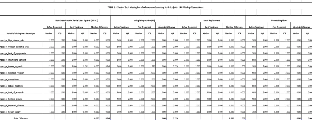
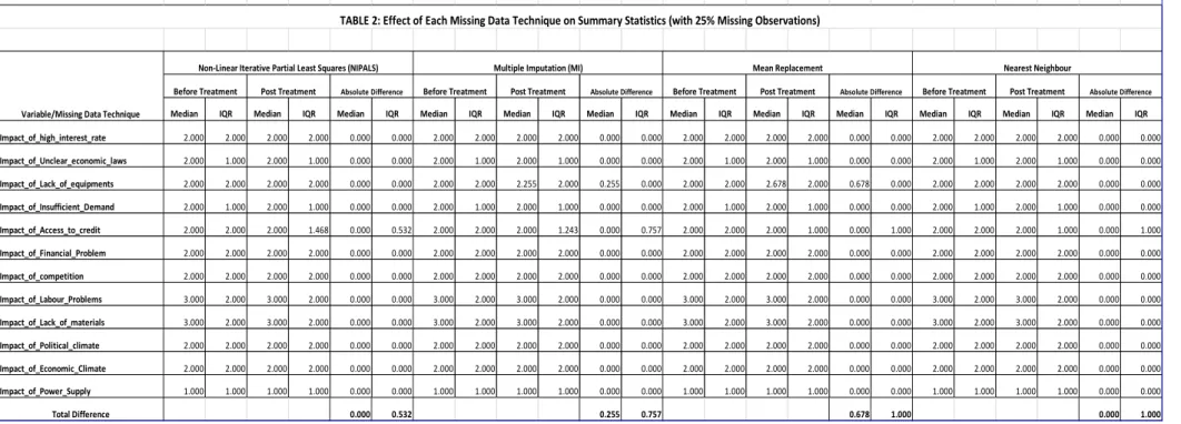
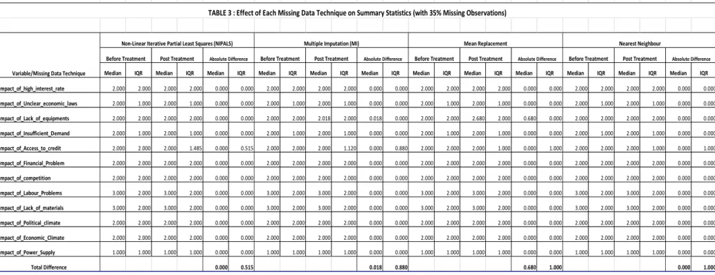
Firstly, we will generate some summary statistics and the disjunctive table, which will show
the proportion of the 1,849 respondents that answered each of the five possibilities of the
likert scale for the 12 constraints. Given the responses provided by respondents for each of
the 12 constraints (variables), a disjunctive table will associate to each of the initial complete
data sets a vector:
[𝑛
01
, 𝑛
02
, … , 𝑛
05
, … 𝑛
060
]
where n
01
represents the number of respondents that choose the first modality for the first
question, n
05
represent number of respondents that choose the last modality for the first
question and n
060
represent number of respondents that choose the last modality for the last
question.
Then, using a completely randomize scheme (table of random numbers) we will exclude 15,
25 and 35 percent of responses, respectively, as if they were item non-response and proceed
to replace them with the various imputation technique. For this project, the following
imputation technique would be employed:
i.
Non-linear Iterative Partial Least Squares
(NIPALS)
ii.
Multiple Imputation (MI)
19
iv.
Nearest Neighbour
After imputation for each of the proportion of missing observation, we would re-compute
the summary statistics and the disjunctive table of the derived data sets and and the result
compared with those of the original data sets.
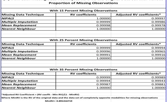
To evaluate relative performance of the various missing data imputation, the data matrice
from each imputation technique and disjunctive tables would be compared using the RV
coefficient. The coefficient made popular by the works of Escoufier, Y (1973) and Robert, P
and Escoufier, Y.
(1976)
, measures similarity between two datasets/matrices such that a
value of 1 indicates complete similarity and 0 indicates complete dissimilarity. This
coefficient, which is a generalization of the square of Spearman
’s
correlation coefficient will
be used to recommend the best imputation technique for the data set.
Following Robert, P and Escoufier, Y.
(1976), if
X (n
×
p) and Y (n
×
p) corresponding to two
matrices of sets of observation from the same n individuals. Then the RV coefficient as a
measurement of the closeness/similarity between X and Y is define as:
𝑅𝑉(𝑋, 𝑌) =
𝑡𝑟(𝑋𝑋
𝑇
𝑌𝑌
𝑇
)
√𝑡𝑟(𝑋𝑋
𝑇
)
2
𝑡𝑟(𝑌𝑌
𝑇
)
2
(1)
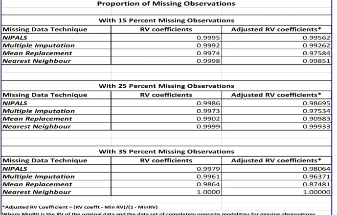
Due to the inherent low variabilities in the responses and those likely to be predicted by the
various imputation technique for the missing values, we expect to have very high RV
coefficients (very close to 1). In a bid to address this issue, this project will go a step further
by generating a better discriminating coefficient which we will call, RV (adjusted).
To do this, we will introduce a control quantity tagged, MinRV(X,Y). MinRV(X,Y) is the value
of the RV coefficient when you replace each missing data by a modality most different from
the true response. That is, if R(n,p) represent the matrix of the true responses, we will define
a certain O(n,p) as the matrix of opposite modalities completely different from the true
response whose element are defined as follows:
𝑂
𝑖
(𝑛, 𝑝) = {
5 𝑖𝑓 𝑅
𝑖
(𝑛, 𝑝) < 3 (𝑚𝑜𝑠𝑡 𝑑𝑖𝑓𝑓𝑒𝑟𝑒𝑛𝑡 𝑓𝑟𝑜𝑚 1 𝑜𝑟 2)
3 𝑖𝑓 𝑅
𝑖
(𝑛, 𝑝) = 3 (𝑖𝑛𝑡𝑒𝑟𝑚𝑒𝑑𝑖𝑎𝑡𝑒 𝑣𝑎𝑙𝑢𝑒)
1 𝑖𝑓 𝑅
𝑖
(𝑛, 𝑝) > 3 (𝑚𝑜𝑠𝑡 𝑑𝑖𝑓𝑓𝑒𝑟𝑒𝑛𝑡 𝑓𝑟𝑜𝑚 4 𝑜𝑟 5)
(2)
20
𝑀𝑖𝑛𝑅𝑉(𝑅, 𝑂) =
𝑡𝑟(𝑅𝑅
𝑇
𝑂𝑂
𝑇
)
√𝑡𝑟(𝑅𝑅
𝑇
)
2
𝑡𝑟(𝑂𝑂
𝑇
)
2
(3)
Finally, we will define the RV(adjusted) as follows:
𝑅𝑉(𝑎𝑑𝑗𝑢𝑠𝑡𝑒𝑑) =
(𝑅𝑉(𝑋, 𝑌) − 𝑀𝑖𝑛𝑅𝑉(𝑅, 𝑂))
(1 − 𝑀𝑖𝑛𝑅𝑉(𝑅, 𝑂))
(4)
Where RV(X,Y) is similar to that generated by equation (1) - for comparing both the
complete data sets and the disjunctive tables and MinRV(X,Y) is as defined in equation (3).
The RV(
adjusted
) will provide a better discriminating factor in order to judge the
performance of the four (4) missing data imputation procedure that is to be undertaken.
The issue of generating non-integer values to replace the missing values by any of the
selected imputation technique (ie values with decimal values) considered distinct from the
five(5) possible modalitie of 1-5 available to respondents are addressed through the
following transformation on the predicted values:
𝑇𝑟𝑢𝑒 𝑃𝑟𝑒𝑑𝑡(𝑋
𝑖𝑗
) = {
𝑁𝑒𝑥𝑡 𝐼𝑛𝑡𝑒𝑔𝑒𝑟 (𝑝𝑟𝑒𝑑𝑡(𝑋
𝑖𝑗
), 𝑖𝑓 𝑝𝑟𝑒𝑑𝑡(𝑋
𝑖𝑗
) < 5
5 𝑖𝑓 𝑖𝑛𝑡𝑒𝑔𝑒𝑟 𝑝𝑎𝑟𝑡 𝑜𝑓 𝑝𝑟𝑒𝑑𝑡(𝑋
𝑖𝑗
) = 5
(5)
Considering the nature of the data sets used for the project (ordinal variables), summary
statistics such as mean and standardard deviation would not provide sufficient information
on the distribution of the choice of 1-5 available to respondents. Inplace of the mean and
stardard deviation, we will be considering the evolution of median and inter-quartile range
(IQR) of each variables. The IQR is a robust measure of dispersion that can tell if reponses for
each variable are closed or scattered across all the range of possibilities of 1-5.
To undertake the MCA, let
𝐷
𝐼
be a diagonal matrix which gives weights associated to each
respondent
𝐷
𝐼
=
1
𝑛
𝐼
𝑛
where n represent sample size and
𝐼
𝑛
the identity matrix. Let
𝐷
𝑗
denote a diagonal matrice which gives weight associated to each item of the
BES:
𝐷
𝑗
= (
𝑓
1
⋯ 0
⋮
⋱
⋮
0 ⋯ 𝑓
60
21
Where
∑
60
𝑗=1
𝑓
.𝑗
= 1
and
𝑓
.𝑗
is the proportion of respondents that have chosen a certain
modality
j
(j=1,2,...,60). If
𝑛
𝑗
represent total number of respondents choosing
modalities
j
then
𝑓
.𝑗
=
𝑛
𝑗
12𝑛
. Let also X be the table of frequencies obtained from the
disjunctive table diving all cells by 12n. It can be shown that PCA associated to the cluster of
respondents is obtained diagonalizing matrice
(′𝑋𝐷
𝐼
−1
𝑋𝐷
𝑗
−1
)
:
(′𝑋𝐷
𝐼
−1
𝑋𝐷
𝐽
−1
)µ
𝑘
= 𝜆
𝑘
µ
𝑘
(7)
Where
λ
𝑘
is eigenvector of such matrice and
µ
𝑘
is the associated eigenvector which
generate K principal axe. From
µ
𝑘
we can easily obtain principal components of the cluster J
related to the answers of the questionnaires (60x1):
𝑌
𝐽
𝑘
=
1
√λ
𝑘
𝐷
𝐽
−1
𝜇
𝑘
(8)
So we will get a configuration of modalities of 12 constraints on a lower dimension space
using the table:
𝑌
𝑗
0= [𝑌
𝑗
01
, 𝑌
𝑗
02
, … … … . , 𝑌
𝐽
0
𝑞
].
Where q is the number of eigen values retained
and
𝑌
𝐽
𝑜