Abstract—This paper is dealing with the problem of tissue characterization of the plaque in the coronary arteries by processing the data from the intravascular ultrasound catheter. Two similarity-based methods are proposed in the paper, namely the histogram-based and the center-of-gravity-based method. Both of them use the general computational strategy of the moving window with fixed size and maximal overlapping ratio. The obtained similarity results are graphically displayed in two modes: hard decision with a given threshold and soft decision with gradual changes in the dissimilarity values.
Simulation results from the tissue characterization of two real data sets - training and test data set, are shown and discussed in the paper with suggestions for further improvement of the method.
Index Terms — moving window, similarity analysis, tissue characterization, normalized histogram, intravascular ultrasound.
I. INTRODUCTION
HE coronary arteries play vital role for the normal functioning of the human heart by supplying fresh blood to the muscular tissue of the heart. Therefore a gradual build-up of a plaque in the inner surface of the artery could lead in some circumstances to severe heart diseases (acute coronary syndrome) such as myocardial infarction and angina.
The inner structure of the plaque tissue is directly related to the risk of a heart failure. The most important are two types of structures in the plaque, namely the lipid and the fibrous
structure. A plaque prone to collapse usually has a large lipid core covered by a thin and small fibrous cap. This condition is very likely to cause breaking of the fibrous cap, which allows the lipid core to enter the blood stream and create dangerous blood clots. Therefore it is of utmost importance to analyze the structure of the plaque and find out the so called lipid and fibrous regions of interest, abbreviated as Lipid ROI and Fibrous ROI.
This work was supported by the Grant-in-Aid for Scientific Research (B) of the Japan Society for Promotion of Science (JSPS) under the Contract No. 23300086.
Gancho Vachkov is with the Graduate School of Science and Engineering, Yamaguchi University, 1677-1 Yoshida, Yamaguchi 753-8512, Japan. (e-mail: [email protected]).
Eiji Uchino is with the Graduate School of Science and Engineering, Yamaguchi University, 1677-1 Yoshida, Yamaguchi 753-8512, Japan. (e-mail: [email protected]), and also with the Fuzzy Logic Systems Institute, 630-41 Kawazu, Iizuka, Fukuoka 820-0067, Japan.
Satoshi Nakao is an undergraduate student in the Faculty of Physics and Information Sciences, Yamaguchi University, 1677-1 Yoshida, Yamaguchi 753-8512, Japan (e-mail: [email protected]).
The analysis and estimation of the size shape and location of the Lipid ROI and Fibrous ROI is usually called tissue characterization in medical terms, which falls into the research area of pattern recognition and pattern classification.
One of the most frequently used techniques to get reliable information from the coronary artery for further visualization and tissue characterization is the Intravascular Ultrasound
(IVUS) method [1]. The IVUS method uses a small rotating catheter with a probe inserted into the coronary artery that emits a high frequency ultra-sonic signal to the tissue. The reflected radio-frequency (RF) signal is measured and saved in computer memory for further analysis and visualization.
The IVUS is essentially a tomographic imaging
technology, in which the reflected RF signal is preprocessed to produce a gray-scale image with a circular shape, called a
B-mode image that is used by medical doctors for observation and analysis of the artery occlusion. One B-mode image corresponds to one cross-section of the coronary artery with a given depth-range in all 256 directions (angles) of rotation of the IVUS probe.
In this paper we do not have a special interest in data visualizing, but rather in the appropriate data analysis for tissue characterization. Therefore we represent the data and the respective results in a rectangular X-Y shape, instead of in circular shape. The axis X denotes the angle (direction) of the IVUS probe within the range of [0,255], while the ordinate Y
denotes the depth of the measurement. i.e. the distance
between the probe and the current measured signal. The depth-of-interest in our investigations is within the range: [0, 400] since any lipid ROI found in the deeper inner areas of the coronary artery is considered as “not so risky”.
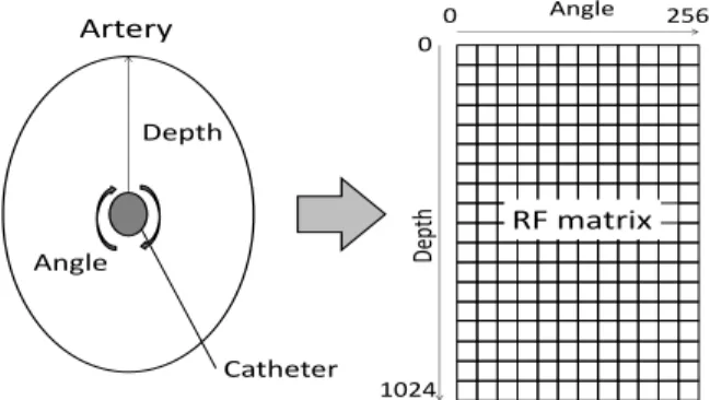
A graphical illustration of the matrix-type information obtained by the IVUS probe is presented in Fig. 1. The obtained large size matrix is called RF matrix and is further on saved in the computer memory It consists of every single measurement obtained for the IVUS probe for one cross section in the coronary artery..
A long term research and data analysis have been done until now [1] – [4] to utilize the information obtained from the IVUS method for a proper tissue characterization of the plaque in the coronary artery. As a result, different classification techniques and algorithms have been proposed, developed and used for various simulations and comparisons. However, currently no “ideal” and easy-to-apply method still exists.
Moving Window-Based Similarity Analysis and
Its Application to Tissue Characterization of
Coronary Arteries
Gancho Vachkov, Eiji Uchino, and Satoshi Nakao
Depth
Angle
Angle
Dep
th
Catheter 0
1024
0 256
Artery
RF matrix
Fig. 1. Information obtained from the IVUS probe for one cross-section of the coronary artery. This is a rectangular X-Y matrix of data with X denoting the rotation angle and Y denoting the depth of the measurement.
In this paper we propose two similarity-based tissue characterization methods. Both of them are based on the same general concept of the moving window computation, but use different methods and models for similarity analysis, namely the histogram-based method and the center-of-gravity method. The work in this paper is a more advanced step of our previous results in [4] that also use the concept of moving window and similarity analysis. In this paper we present a moving window with maximal overlapping ration and a new method for similarity analysis.
The rest of the paper is organized as follows. In Section II the general concept of the moving window, combined with different similarity analysis methods is presented. Section III explains two models used for similarity analysis and Section IV gives details about the similarity analysis calculations. Section V shows and explains the tissue characterization results obtained by using the two different methods. Finally, Section VI concludes the research results in this paper.
II. THE MOVING WINDOW-BASED SIMILARITY ANALYSIS A. The General Moving Window Approach
We propose here a general Moving Window approach to similarity analysis, which was tested and shown to be a suitable and practical tool for solving the problem of tissue characterization of the coronary artery plaque. A graphical explanation of this approach is given in Fig. 2.
max
D y
N
x
N
One step movement255
Fig. 2. The general concept of the Moving Window approach to similarity analysis. The fixed-size window scans the entire rectangular area of data from the top-left corner (angle 0 and depth 0) to the bottom-right corner (angle 255, depth = Dmax) , with one step at a time.
First of all, the rectangular RF data matrix that corresponds to the whole examination area of one cross section of the artery is extracted. This matrix consists of all
the values of the reflected RF signal and has a size of 256 x
Dmax, with the value of Dmax = 400 considered as a
sufficient maximal depth for examination.
The next preparation step is to select a rectangular window
with size NXNY, with the following “reasonable” values for the Angle_Range: 2NX60 and for the Depth_Range: 5NY100.
The window with the predefined size performs scanning of the whole data matrix, starting from the upper-left corner to the bottom-right corner of the matrix. At each step, the window is shifted just one angle position to the right until the end of the current horizontal line. After that the window returns to its leftmost angle position, but is shifted one depth
position below and resumes the scan to the right of the data RF matrix. This process is continued until the window reaches the bottom-right corner of the data matrix.
It is worth noting that in such way, every two neighboring windows are overlapped with a maximal overlapping ratio, because they differ from each other by only one position. This way of movement of the windows is different from our previous moving window approach in [4] where no overlapping between the neighboring windows was assumed. Our assumption was that by using the maximal possible overlapping ratio, better classification (characterization) results could be achieved. Such assumption has been later on proven experimentally to be true.
For the proposed moving window approach with maximal overlapping ratio, it is calculated that the following large number of windows will be generated during the whole scanning:NW256(DmaxNY1).
B. Similarity Analysis by Using the Moving Window
We define here the similarity analysis as a method for comparing in a numerical way the structure (characteristics) of two data sets. The first data set is usually fixed (constant) and corresponds to a given region of interest, such as Lipid
ROI or Fibrous ROI. The second data set is generated (extracted) from the current window W ii, 1, 2,...,NW during the Moving Window process.
Therefore the similarity analysis is essentially a supervised procedure for decision making, in which the so called Dissimilarity Degree DS is calculated between the given data sets. The value of DS is usually bounded:DSi[0, ]T and shows how close is the data structure from the current window W ii, 1, 2,...,NW to the data structure in the predefined ROI. Then, a value of dissimilarity, close to zero suggests that the two data sets are very similar and a bigger value (closer to T) stands for a bigger difference (bigger discrepancy) between the two data sets. For the purpose of fair quantitative comparison between the data sets, the dissimilarity value is often normalized as:DSi[0,1].
When using the similarity analysis in the frame of the moving windows approach, the similarity value DSi will be calculated many times, namely for each current position of the window Wi. Then the natural question is where (at which location) to assign the currently calculated value of DSi? This problem arises because all NXNYdata in the current window Wi have been used for calculation of the dissimilarity.
In this paper we take the following decision, namely the
same dissimilarity degree DSi will be assigned to all coordinates (all cells) within the window Wi that have been used in the calculations. In order to keep in a memory all these values, we create a new rectangular matrix called
Dissimilarity Matrix DM, with the same dimension as the Data Matrix RF, i.e. 245 x Dmax.
It is easy to realize that each data item (each cell) in the original data matrix RF will be visited many times by the moving window. If N denotes the number of all visits of a given cell at location { , };i j i[ ,0 255]; j[ ,0 Dmax] by a
moving window with sizeNXNY, then this number is calculated as:
max
max max max
( ) , 0 ;
, ;
( ) , ;
Y Y
X Y Y Y
Y Y
N j 1 N if j N 2
N N N if N 1 j D N 1
N D j 1 N if D N 2 j D
(1)
The DM matrix is actually an additive matrix that accumulates all the calculated values for the dissimilarity degrees at the same location {i,j}, as follows:
, ,...,
i j i j k
dm dm DS k 1,2 N
(2) Finally, the true dissimilarity degree for this {i,j} location is taken as a mean value of the accumulated similarity degrees in DM, namely:
max
/ , [ , ]; [ , ]
i j i j
dm dm N i 0 255 j 0 D
(3) Now all true dissimilarity degrees are saved in the DM matrix and are ready to be displayed in at least two different ways for the final decision making.
A Hard Decision making. It applies a user-defined
threshold Th for separation of all the values into 2
crisp classes, namely: Similar (with dmi jTh) and
Not Similar (with dmi jTh) to the respective
reference region of interest, such as Lipid ROI or
Fibrous ROI. Then the Similar only class can be visualized in an easy-to-see way to the medical doctor for his final decision. Here it is worth noting that the proper selection of the threshold is not an easy task, which can lead sometimes to ambiguous results. A Soft Decision making. It is a kind of fuzzy way of
displaying the results, in which all calculated values in (3) are visualized with different color intensity. The values closer to zero are shown in an easy-to-notice
darker color. Reversely, the areas containing larger values of dissimilarity degrees will be shown in very
thin (or almost white) color and can be neglected by the final doctor’s decision.
III. MODELS USED FOR SIMILARITY ANALYSIS
Before calculating the similarity analysis between two data sets, we have to decide what type of model would be best suited for describing the data structure. Then, according to the illustration in Fig. 3., we have to compute (once only) the
Reference Models RMLandRMFfor the predefined Lipid ROI and Fibrous ROI., by using their respective data: ML and MF.
One window Lipid ROI Fibrous ROI
Dep
th
0
0 255
Fig. 3. Illustration of three different data sets to be compared by the similarity analysis. One is the data set from the Lipid ROI, the other is the data set from the Fibrous ROI and the shadowed rectangular data set belongs to the current moving window. All these data set use the same type of model for structure representation.
After that another model calculation is needed for each of the moving windows, by using the data MWNXNY contained in this window.
In this section we explain two simple types of models, which are convenient for similarity analysis and therefore used in further simulations and experiments.
A. The Normalized Histogram (NH) Model
This model represents the normalized distribution of the RF signal intensity (strength) within the whole range of intensities [ ,0 Rmax]. If M denotes the data number in a given
ROI or in a given window W and N is the number of the pre-selected intervals with equal width , then the normalized histogram is calculated as follows:
1
/ [0,1]; 1
N
i i i
i
h m N h
(4)where
m i 1,2
i,
,...,
N
denotes the number of measured RF intensities within the i-th interval. Here the following conditions hold:
1
0
;
N
i i
i
m
M
m
M
(5)Fig. 4. The raw reflected RF signal at one fixed angle (100) of the IVUS catheter and all depths, starting from 0 to 400.
One window Fibrous ROI
i
h
0.15
0.1
0.05
0
1780-1799 1880-1899 1980-1999 2080-2099 2180-2199 Intensity
Fig. 5. Illustration of two histograms and their difference (the shadowed area). The left histogram is obtained from the Lipid ROI and the right histogram is obtained from one arbitrary selected window.
B. The Center-of-Gravity (COG) Model
This model evaluates the structure of a given data set by using two parameters with clear physical understanding, namely the Center-of-Gravity (COG) and the Standard Deviation (SD). Data sets with different structures have different values of COG and SD, so the difference between the two parameters can be used for similarity analysis.
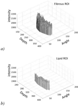
The next Fig. 6. serves as a graphical illustration of two different data structures, namely a Fibrous ROI and a Lipid
ROI, extracted from the original data in the RF matrix, as shown in the example in Fig. 3. It is easy to notice that the Fibrous ROI consists of data (i.e. RF signal intensities) with higher value and bigger variations, that the data from the Lipid ROI, which are lower in values and smoother.
The main reason for such difference is that the lipid tissue is softer and absorbs a large amount of the RF signal, while the fibrous tissue has higher elasticity and as a result reflects
a large part of the signal.
Let M denotes the number of data, i.e. the number of extracted RF signal intensities
R i
i,
1, 2,...,
M
from a given ROI or a given window W. Then the two model parameters COG and SD are easily calculated as follows:- The Center-of-Gravity of the model is simply calculated as a mean value of the one-dimensional RF signal:
1
M
i i
COG
R M
(6)
-The Standard Deviation is calculated as:
2
1
(
)
(
1)
M
i i
SD
R
COG
M
(7)
a)
Fibrous ROI
in
tensi
ty
2200 2100 2000 1900
150 50
100
200 200
250 300
350 400 150
b)
Lipid ROI
in
tensi
ty
150 50
100
200 280
360 400 2200
2100 2000 1900
320 240
280
Fig. 6. Two different 3-dimensional data structures; (a) The data from the Fibrous ROI; (b) The data from the Lipid ROI; The difference can be visually noticed.
The calculated values of COG and SD for the Fibrous ROI and the Lipid ROI, extracted from the experimental RF data matrix are as follows:
Fibrous ROI: COG = 1990.5; SD = 57.90;
Lipid ROI : COG = 1954.7; SD = 17.20. IV. SIMILARITY ANALYSIS CALCULATIONS
As we have already mentioned in Section II, the similarity analysis is based on calculating the Dissimilarity Degree
[0, ]
DS T between two selected data sets. It is obviously
that this calculation would depend on the assumed model for describing the data sets. Since we have assumed two models in Section III, namely the Normalized Histogram (NH) Model and the Center-of-Gravity (COG) Model, the respective calculation of DS is as follows:
A. Dissimilarity Calculation by Use of the NH Model
Basically, it is a comparison of two curves (two histograms) that have been created from two data sets by using (4) and (5). Let
H
0 andH
idenote the normalized histograms of a given ROI and the i-th moving window respectively. Then the normalized value of dissimilarity is calculated as:0 0
1
( , ) 2 [0,1]
N i
i i j j
j
DS DS H H h h
(8)The denominator of 2 is used, because the largest possible discrepancy between the two histograms (when they do not overlap at all) will be 2.
B. Dissimilarity Calculation by Use of the COG Model
We assume here the easiest and the most practical way for comparing the two data sets, by calculating the Euclidean
0
2 2
0 0 max
( , )
( ) ( ) [0, ]
i i
i i
DS DS M M
COG COG SD SD T
(9)
Since the maximal distance
T
max is usually data dependentvalue, the original dissimilarity (9) is not normalized between 0 and 1 .However, it is possible to make some specific practical assumptions, in order to curb the
non-interesting high vales of dissimilarity and to display anly the similarities closer to zero (i.e the most interesting cases).
V. SIMULATION RESULTS FROM TISSUE CHARACTERIZATION A. Simulation Details and Conditions
The above described moving window approach for similarity analysis was used for tissue characterization of several sets of real data, in the form of respective RF matrices, each of them with X-Y size: 256 x 400 (the maximal depth:
Dmax = 400). For each matrix, the respective Lipid ROI and
Fibrous ROI have been properly identified and marked by a medical doctor through a microscopic analysis. These ROI data were used for creating the Reference Lipid and Fibrous models for similarity analysis and also for testing and analyzing the correctness of the simulation results.
In all the simulations, a moving window with fixed-size of
30 x 40 was used, which means that totally 92426 windows were generated and used for similarity analysis. Despite the large number of the windows, the calculations were relatively fast, because of the simple structure of the proposed NH and COG models. The CPU time for all RF sets did not exceed 40 sec. This fact suggests that if the proposed tissue characterization method is “accurate enough”, it could be applied in near real-time mode.
B. Simulation Results from the Training Set
First, we used one RF set as a Training Set for obtaining the Reference models for the Fibrous and Lipid ROI. Here both models were calculated, namely the NH and the COG model. They were used for similarity analysis with two types of decisions: Hard decision and Soft decision, as described in Section II with user defined thresholds. The results are shown in the following 4 figures: Fig. 7, 8, 9 and 10.
It is easy to notice that the characterization results show much larger areas for both Lipid and Fibrous ROI than the actual identified ROI by the doctor. There could be different reasons for such “far from ideal” results. One of them is
“hidden” in the threshold choice and the other is that the doctor actually identified one only ROI and did not check for existence of other ROI within the sane cross section.
a) 0
400 350 300 250 200 150 100 50
250 0 50 100 150 200
Fibrous
b) 0
400 350 300 250 200 150 100 50
250 0 50 100 150 200
Lipid
Fig. 7. Hard-Decision Results from the tissue characterization of the Fibrous (a) and Lipid (b) ROI by using the Histogram-based Model (NH). The threshold used is: Th = 0.2.
a) 0
400 350 300 250 200 150 100 50
250 0 50 100 150 200
Fibrous
b) 0
400 350 300 250 200 150 100 50
250 0 50 100 150 200
Lipid
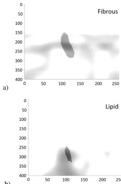
Fig. 8. Soft-Decision Results from the tissue characterization of the Fibrous (a) and Lipid (b) ROI by using the Histogram-based Model (NH). The threshold used is: Th = 0.2.
a) 0
400 350 300 250 200 150 100 50
250 0 50 100 150 200
Fibrous
b) 0
400 350 300 250 200 150 100 50
250 0 50 100 150 200
Lipid
a) 0
400 350 300 250 200 150 100 50
250 0 50 100 150 200
Fibrous
b) 0
400 350 300 250 200 150 100 50
250 0 50 100 150 200
Lipid
Fig. 10. Soft-Decision Results from the tissue characterization of the Fibrous (a) and Lipid (b) ROI by using the COG Model with a threshold used: Th = 30.
C. Simulation Results from a Test Data Set
In order to test the reliability of the proposed methods for tissue characterization, we need another data set that has not been used for training, but for which we “know the answer”. Therefore we selected another RF matrix from our available experimental data and used it as a Test Data set. When calculating the results for tissue characterization of this new Test Data set, we used the same NH and COG ROI models, which were created from the previous Training Data set. And since we know the actual and properly identified Lipid and Fibrous ROI for the Test Data set, it was possible to make visual estimation of the characterization results.
Because of space limitation in this paper, we present here the soft decisions only, for both models - the NH and the COG model. The results are seen in Fig. 11 and Fig. 12.
a) 0
400 350 300 250 200 150 100 50
250 0 50 100 150 200
Fibrous
b) 0
400 350 300 250 200 150 100 50
250 0 50 100 150 200
Lipid
Fig. 11. Soft-Decision Results from the tissue characterization of the Fibrous (a) and Lipid (b) ROI by using the Normalized Histogram-based Model (NH). The threshold used is: Th = 0.3.
a) 0
400 350 300 250 200 150 100 50
250 0 50 100 150 200
Fibrous
a) 0
400 350 300 250 200 150 100 50
250 0 50 100 150 200
Lipid
Fig. 12. Soft-Decision Results from the tissue characterization of the Fibrous (a) and Lipid (b) ROI by using the COG Model with a threshold used: Th = 30.
As seen from these figures, the characterization results are similar as quaity to the results from the Trainig Data set.
VI. CONCLUSION
We proposed in this paper a general Moving Window computational approach with maximal overlapping ratio for tissue characterization of coronary arteries. This approach uses data obtained from the IVUS catheter and allows implementation of different methods and models for similarity analysis. Two of them, the Normalized-Histogram based and the Center-of-Gravity based models were proposed and used in the paper. They calculate the dissimilarity degree
DS for taking the final characterization decision, which can be visualized in two forms, namely as Hard or Soft decision.
The simulation results by using Training and Test Data sets show positive, but still “far from perfect” results. They usually detect a large part of the actual Lipid and Fibrous ROI, but at the same time show also some other areas, as “looking very similar” to those ROI. Therefore further improvements of the proposed methods are needed.
Possible further improvements include optimization of the window size and the threshold for decision making, as well as constructing some different methods for similarity analysis and for calculation of the dissimilarity degree.
REFERENCES
[1] C. De Korte, H. G. Hansen and A. F. Van der Steen, "Vascular ultrasound for atherosclerosis imaging," Interface FOCUS, vol. 1, pp. 565-75, 2011. [2] E. Uchino, N. Suetake, T. Koga, R. Kubota et al., “Fuzzy Inference-based plaque boundary extraction using image separability for IVUS image of coronary artery”, Electronic Letters, vol.45, no. 9, pp. 451-453, 2009. [3] T. Koga., S. Furukawa, E. Uchino and N. Suetake, “High-Speed
Calculation for Tissue Characterization of Coronary Plaque by Employing Parallel Computing Techniques”, Int. Journal of Circuits, Systems and Signal Processing, vol. 5, No. 4, pp. 435-442, 2011. [4] G. Vachkov and E. Uchino, “Similarity-based method for tissue
characterization of coronary artery plaque”, in CD-ROM Proc.24th Annual Conference on Biomedical Fuzzy Systems Association (BMFSA), pp. 257-260, Oct. 29-20, 2011.