Invariance analysis and similarity solution of heat transfer for MHD viscous power-law fluid over a non-linear porous surface via group theory

Volume , )ssue : pp.

6-Available online at www.ijaamm.com ISSN: 2347-2529

Invariance analysis and similarity solution of heat transfer

for MHD viscous power-law fluid over a non-linear porous

surface via group theory

R. M. Darji a, ∗ and M. G. Timol b

a

Department of Mathematics, Sarvajanik College of Engineering and Tecchnology,Surat-1, India

b

Department of Mathematics, Veer Narmad South Gujarat University, Surat-7, India

Received 17 September 2013; Accepted (in revised version) 21 November 2013

A B S T R A C T

In this paper general group symmetry analysis so-called deductive group-theoretical method is applied to analyze the boundary layer flow of electrically conducting viscous fluid over with heat transfer over a non-linear surface. The symmetry groups admitted by the corresponding boundary value problem are obtained. With the use of the entailed similarity transformations the governing equations reduce to a set of non-linear ordinary differential equations. The system of equations is solved numerically using MATLAB coding. The effect of various flow parameters is studied for both Newtonian and Non-Newtonian power-law fluids in case of stretching and shrinking sheet.

Keywords: Deductive symmetry groups, power-law fluid, MHD, boundary-layer flow, MATLAB.

MSC 2010 codes:76A05, 76M55, 54H15.

© 2013 IJAAMM

1 Introduction

boundary layer equations are especially interesting from a physical point of view because they have the capacity to admit number of invariant solutions.

In this paper, we apply the so-called deductive group symmetry method (Darji and Timol 2013) for a particular problem of boundary layer theory. The main advantage of such method is that they can successfully be applied to non-linear differential equations. The symmetries of a differential equation are those continuous groups of transformations under which the differential equation remains invariant, that is, a symmetry group maps any solution to another solution. The interesting point is that, having obtained the symmetries of a specific problem, one can proceed further to find out the group-invariant solutions, which are nothing but the well-known similarity solutions. The similarity solutions are quite popular because they result in the reduction of the independent variables of the problem. In our case, the problem under investigation is two-dimensional. Hence, any similarity solution will transform the governing system of PDEs into a system of ODEs. Most of the researchers in the field of fluid mechanics try to obtain the similarity solutions by introducing a general similarity transformation with unknown parameters into the differential equation obtaining in this way an algebraic system. Then, the solution of this system, if exist, determines the values of the unknown parameters. In our opinion, it is better to attack any problem of similarity solutions from the outset, i.e, to find out the full list of the symmetries of the problem and then to study which of them are appropriate to provide group-invariant (or more specifically similarity) solutions. To obtain symmetry of a differential equation is equivalent to the determination of the transformation group associated with this symmetry. In [Olver (1993), Bluman and Kumei (1989), Ibragimov (1985, 1999)], one can find the general theory of Lie groups as well as the implied methods for determining transformation group via the infinitesimal generator components. An alternative way being based on exterior calculus for determining the transformation group so-called deductive group can be found in Moran and Gaggioli (1968). It is worth noting that there is an extensive literature where the methods arising from exterior calculus are used to attack symmetry problems of continuum mechanics [Suhubi (1991, 1994), Pakdemirli and Suhubi (1992), Kalpakides (1998, 2001), Koureas et. al (2001, 2003)].

The problem in the reverse case i.e., very little is known about the shrinking sheet where the velocity on the boundary is towards the origin or a fixed point, and the unsteady shrinking film solution was first investigated by Wang (1990). Again, Miklavcic and Wang (2006) studied the viscous hydrodynamic flow over a shrinking sheet for both two-dimensional and axisymmetric flows. It is also noted that the mass suction at the wall is required generally to maintain (or smooth) the flow over a shrinking sheet. They discussed the proof of existence and (non) uniqueness of both exact numerical and closed form solutions. The analysis of Miklavcic and Wang (2006) was also extended in various directions for different fluids by many researchers. Recently, Fang (2008) investigated the boundary layer flow over a shrinking sheet with surface moving with power-law velocity. A theoretical analysis is carried out for different values of power-index of the surface velocity using exact and numerical solutions. These studies restrict their analyses to Newtonian fluids. Flow due to a stretching sheet also occurs in thermal and moisture treatment of materials, particularly in processes involving continuous pulling of a sheet through a reaction zone, as in metallurgy, textile and paper industries, in the manufacture of polymeric sheets, sheet glass and crystalline materials. It is well known that a number of industrial fluids such as molten plastics, polymeric liquids, food stuffs or slurries exhibit Non-Newtonian character. Therefore a study of flow and heat transfer in non-Newtonian fluids is of practical importance.

In recent years several industries deal with the Non-Newtonian fluids under the influence of magnetic field. In view of this, some researchers [Sarpakaya (1961), Saponkov (1967), Martinson and Pavlov (1971), Samokhen (1987), Andersson et. al (1992), Cortell (2005a), Liao (2005)] have presented works on MHD flow and heat transfer in an electrically conducting power law fluid over a stretching sheet. Motivated by this, we produce similarity analysis via deductive group method based on general group transformation is, probably first time, to derive symmetry group and similarity solutions for boundary layer flow of an electrically conducting power-law fluid over non-linear surface. The aim of the present work is twofold: first to derive systematically the similarity transformation using general group theoretic method under similarity requirement for the governing equations, secondly to incorporate the effects of applied magnetic field for an electrically conducting fluid and to carry out the heat transfer analysis.

2 Mathematical

formulation

Consider a two-dimensional flow of an incompressible viscous fluid past a porous non-linear surface (stretching/shrinking sheet) at y =0. The stretching/shrinking velocity of the sheet is

( )

r

w

u x =cx , where c>0, c<0 respectively for stretching and shrinking sheet (referred as stretching/shrinking parameter), r is power-law velocity index and the wall mass suction velocity is v_w =v_w

( )

x . The x-axis is taken along the stretching/shrinking sheet and the y-axis perpendicular to it into the fluid. The fluid is electrically conducting and the magnetic field

( )

Also for the power fluid, the rheological equation of state between the stress components τ_ij and the strain components e_ij, is defined by (Vujanovic et al. 1972 )

1 2 n

ij P ij K e elm lm eij

τ δ

−

= − +

∑∑

where P is the pressure, δ_ijis the Kronecker delta and K and n are consistency and flow behavior indices of the fluid respectively. Such fluids are known as Non-Newtonian power- law fluids and n is referred as the power law index. When n>1the fluid is described as dilatant, n<1pseudo-plastic and when n=1 it is simply the Newtonian fluid.

Under boundary layer approximation, the continuity, momentum, and energy equations are 0,

u v

x y

∂ ∂

+ =

∂ ∂

(1)

( )

1 2

,

n

B x

u v u u

u v u

x y y y y

σ ν ρ − ⎛ ⎞ ∂ ∂ ∂ _⎜ ∂ ∂ _⎟ + = − ⎜ ⎟

∂ ∂ ∂ _⎝ ∂ ∂ _⎠ (2)

2 2

2

p

T T T u

C u v

x y y y

ρ ⎛_⎜ ∂ + ∂ _⎟⎞=α ∂ +µ⎛_⎜∂ ⎞_⎟

∂ ∂ ∂ ∂

⎝ ⎠ ⎝ ⎠ (3)

where u and v are the velocity components, x and y are the space coordinates, T is the temperature, νis the kinematic viscosity of the fluid, α _{is the thermal diffusivity of fluid,} ρ is the density of the fluid, C_p is the specific heat at constant pressure of the fluid. In (2), the external electric field and the polarization effects are neglected

The boundary conditions for the problem are:

( )

,

( )

, 0, at 0

0, as

w w

u u x v v x T T y

u T T_∞ y

= = = = ⎫

⎬

→ → → ∞_⎭ (4)

Introducing following non-dimensional quantities:

* , * , * , * , *

w

x y u v T T

x y u v

L L U U θ T T

∞

∞

−

= = = = =

− (5)

U is the free stream velocity and L is the characteristic length.

Substituting the values (1) to (4) and dropping the asterisks (for simplicity) yields the following dimensionless equations,

0

u v

x y

∂ ∂

+ =

1 ₂

2

n

u v u u

u v n Mu

x y y y

−

⎛ ⎞

∂ ∂ ∂ ∂

+ = _{⎜ ⎟} −

∂ ∂ ⎝∂ ⎠ ∂ (7)

2 2 2 1 Pr u u v

x y y y

θ θ θ

λ⎛ ⎞

∂ ∂ ∂ ∂

+ = + _{⎜ ⎟}

∂ ∂ ∂ _⎝∂ _⎠ (8)

where

( )

2 B x

M σ

ρ

= is the magnetic field strength, Pr ρ νCp

α

= is the Prandtl number and

2

2 U L µ

λ= is the flow parameter.

Introducing the stream function ψ , which is related to the components of velocity field such that u , v

y x

ψ ψ

∂ ∂

= = −

∂ ∂ , above system of PDEs reduce to:

1

2 2 2 3

2 2 3

n

n M

y y x x y y y y

ψ ψ ψ ψ ⎛ ψ ⎞ − ψ ψ

∂ ∂ ∂ ∂ ∂ ∂ ∂

− = _{⎜ ⎟} −

∂ ∂ ∂ ∂ ∂ _⎝∂ _⎠ ∂ ∂ (9)

2

2 2

2 2

1 Pr

y x x y y y

ψ θ ψ θ θ ψ

λ⎛ ⎞

∂ ∂ ∂ ∂ ∂ ∂

− = + ⎜_⎜ ⎟_⎟

∂ ∂ ∂ ∂ ∂ _⎝∂ _⎠ (10)

The associated boundary conditions can be written as,

(

)

( )

(

)

( )

(

)

( )

(

)

(

)

, 0 , , 0 , , 0

, 0, , 0 as

w w w

x u x x v x x x

y x

x y x y y

y ψ ψ θ θ ψ θ ∂ ₌ ∂ _{= =} ⎫ ⎪ ∂ ∂ _⎪ ⎬ ∂ _⎪ → → → ∞ ⎪ ∂ _⎭ (11)

3 Application

The procedure is initiated with the application of the class of a one-parameter continuous deductive group of transformations to the system of PDEs (11) and (12). Under this class, first, we search the subgroup of transformations, through which one will reduce the two independent variables by one and the system of non-linear partial differential equations (11) and (12) will transform to the system of ordinary differential equations.

3.1 Group formulation and invariance analysis

Consider the group C_G, a class of transformation of one-parameter ‘a’of the form:

( )

( )

: Q Q

G

where Q stands for x y, , , ,ψ θ M whereas ℵ' s and ℜ' s are real-valued and are at least differentiable in the real argument a .

To transform the differential equation, transformations of the derivatives of ψ are obtained from C_G via chain-rule operations:

; , , ; , , Q i i i Q i j i j i j

Q Q

Q M i j x y

Q Q

ψ θ

⎫

⎛_ℵ ⎞

=⎜_⎜ ⎟_⎟ ⎪

ℵ ⎪

⎝ ⎠

= =

⎬

⎛ _ℵ ⎞ _⎪

=⎜_⎜ ⎟_{⎟ ⎪}

ℵ ℵ

⎝ ⎠ ⎭

(13)

Now (9) and (10) are said to be invariantly transformed, for some functions

χ

₁

( )

a and

( )

2 a

χ

whenever,

( )

( )

1

2 2 2 3

2 2 3

1

2 2 2 3

1 _{2 2 3}

2 2 2 2 2 2 2 2 ₂ 1 Pr 1 Pr n n n M

y y x x y y y y

a n M

y y x x y y y y

y x x y y y

a

y x x y y y

ψ ψ ψ ψ ψ ψ ψ

ψ ψ ψ ψ ψ ψ ψ

χ

ψ θ ψ θ θ ψ

λ

ψ θ ψ θ θ ψ

χ λ − − ⎛ ⎞ ∂ ∂ ∂ ∂ ∂ ∂ ∂ − − _{⎜⎜ ⎟⎟} + ∂ ∂ ∂ ∂ ∂ _⎝∂ _⎠ ∂ ∂ ⎡ _{⎛ ⎞} ⎤ ∂ ∂ ∂ ∂ ∂ ∂ ∂ ⎢ ⎥ = − − ⎜_⎜ ⎟_⎟ + ∂ ∂ ∂ ∂ ∂ ⎢ ∂ _⎝∂ _⎠ ∂ ⎥ ⎣ ⎦ ⎛ ⎞ ∂ ∂ ∂ ∂ ∂ ∂ − − − _{⎜⎜ ⎟⎟} ∂ ∂ ∂ ∂ ∂ _⎝∂ _⎠ ∂ ∂ ∂ ∂ ∂ ∂ = − − − ∂ ∂ ∂ ∂ ∂ ∂ 2 2 ⎫ ⎪ ⎪ ⎪ ⎪ ⎪ ⎪ ⎪⎪ ⎬ ⎪ ⎪ ⎪ ⎪ ⎪ ⎡ _{⎛ ⎞} ⎤ _⎪ ⎢ _{⎜ ⎟} ⎥ _⎪ ⎜ ⎟ ⎢ _{⎝ ⎠} ⎥ _⎪ ⎣ ⎦ ⎭ (14)

Substituting the values from the (12) and (13) in above system (14), yields

(

)

(

)

(

)

(

)

(

)

( )

1 2

2 _{2 2 2 3}

2 2 2 1 2 3

1

2 2 2 3

1 _{2 2 3}

n n

M M

n y

x _{y y}

n

n M

y y x x y y y y

a n M

y y x x y y y y

ψ ψ

ψ _{ψ ψ ψ ψ ψ ψ ψ}

ψ ψ ψ ψ ψ ψ ψ

χ

−

+

−

⎡ ⎤

⎡_{∂ ∂ ∂ ∂} ⎤ _ℵ ⎛_∂ ⎞ _{∂ ℵ ∂}

ℵ _{⎢ − ⎥− ⎢ ⎜ ⎟ ⎥+ ℵ + ℜ}

⎜ ⎟

∂ ∂ ∂ ∂ ∂ ⎢ ∂ ∂ ⎥ ℵ ∂

ℵ _ℵ ⎣ ⎦ _{ℵ ⎣} ⎝ ⎠ _⎦

⎡ _{⎛ ⎞} ⎤ ∂ ∂ ∂ ∂ ∂ ∂ ∂ ⎢ ⎥ = − − ⎜_⎜ ⎟_⎟ + ∂ ∂ ∂ ∂ ∂ ⎢ _{∂ ⎝∂ ⎠ ∂} ⎥ ⎣ ⎦ (15)

( )

(

)

( )

( )

2 ₂ 2

2 2 4

2 2 2 ₂ 1 Pr 1 Pr

x y _{y y}

u

y x x y y y

u a

y x x y y y

ψ θ _{ψ θ ψ θ} θ _θ ψ

λ

ψ θ ψ θ θ

χ λ

⎡ ⎤

⎡ ⎤

⎡ ⎤ ⎛ ⎞

ℵ ℵ ∂ ∂ ∂ ∂ ℵ ∂ ℵ _⎢ ∂ _⎥

− − ⎢ ⎥− _{⎜ ⎟}

⎢_{∂ ∂ ∂ ∂} ⎥ _∂

ℵ ℵ ⎣ ⎦ _{ℵ ⎣} ∂ _{⎦ ℵ} ⎢_⎣ ⎝ ⎠ ⎥_⎦

The invariance of (15) and (16) together with boundary conditions (11), implies that

(

)

(

)

(

)

(

)

( )

(

)

(

)

(

)

( )

2 2 1

2 2 1

2

2

2 4

0,

.

x y M

n _M

n y

x _{y y}

x y y y a a θ ψ ψ ψ ψ

ψ θ θ _ψ

χ

χ +

⎫

ℜ = ℜ = ℜ = ℜ = ℜ =

⎪ ⎪

ℵ ℵ

ℵ ₌ ℵ _{= = ⎪}

ℵ

ℵ _{ℵ ℵ} ⎬

⎪

ℵ ℵ ℵ _ℵ ⎪

= = = _⎪

ℵ ℵ _{ℵ ℵ ⎭}

(17)

These yields,

(

)

₍

₎

(

)

(

)

3 _{2 2}

2

1

x y _y M _y

y

, ψ , θ

ℵ = ℵ ℵ = _ℵ ℵ = ℵ = _ℵ

ℵ

(18)

Finally, we get the one-parameter group G, which transforms invariantly the differential equations (9) and (10) and the auxiliary conditions (11), as

(

)

(

)

(

)

(

)

3 2 2 2 : : 1 y H y y y y x x G y y G M M ψ ψ θ θ ⎧ _⎧⎪ = ℵ ⎪ _⎨

⎪ _{⎪⎩ = ℵ}

⎪

⎪⎪ _{= ℵ}

⎨ ⎪ = ⎪ ℵ ⎪ ⎪ = ⎪ ℵ ⎩ (19)

3.2 The complete set of absolute invariants

Now we have proceeded in our analysis to obtain a complete set of absolute invariants. If

(

x y,

)

η η= is the absolute invariant of the independent variables then,

(

, , , ,

)

( )

, 1, 2,3

j j

g x yψ M θ = Π η j= (20)

are absolute invariants of dependent variables.

The application of the basic theorem in group theory, [Moran and Gaggioli (1968), Morgan (1952)], states that:

A function g x y

(

, , , ,ψ θ M

)

is an absolute invariant of a one-parameter group if it satisfies the following first-order linear partial differential equation,

(

)

5

1

0, , , , ,

i i i i

i i

g

Q Q x y M

Q

α β ψ θ

=

∂

+ = =

∂

where

0 0

and 1,...5.

i i

i i i

a a

ε ε ε ε

α β

= =

∂ℵ ∂ℜ

= = =

∂ ∂ (22)

and ‘a0’denotes the value of parameter ‘a’ which yields the identity element of the group G. Since ℜ = ℜ = ℜ = ℜx y θ M = ℜ =ψ 0 implies that

β

₁=

β

₂=

β

₃=

β

₄=

β

₅=0 and from (22) we get ₁ 3 ₂ 3 ₃ 3 ₄ 3 ₅

2 2 2

α = α = α = − α = α . Hence, equation (21) reduces to

2 2 2

0.

3 3 3 3

g y g g M g g

x

x y M

ψ θ

ψ θ

∂ ∂ ∂ ∂ ∂

+ + − + =

∂ ∂ ∂ ∂ ∂ (23)

The absolute invariant of independent variables owing the equation (23) is η η=

(

x y,

)

if it satisfies the first order linear partial differential equation

0. 3

y x

x y

η η

∂ ∂

+ =

∂ ∂ (24)

Applying the variable separable method we get,

(

)

1/3

,

x y yx

η = − (25)

Further the absolute invariants of dependent variables owing the (28) are followed by

(

)

2/3

( )

(

)

2/3

( )

(

)

2/3

( )

1 , , 1 , 2 , , 2 , 3 , , 3 .

g x yψ =ψx− = Π η g x y M =Mx = Π η g x y θ =θx− = Π η

Hence,

(

)

2/3

( )

2/3

( )

(

)

2/3

( )

1 2 3

, , , , .

x y x M x x y x

ψ = Π η = − Π η θ = Π η (26)

4 Group invariant solution

Since M x

( )

is independent of y, Π₂

( )

η must be constant say m. (Referred as magnetic field parameter)

Thus, finally we get the complete set of absolute invariants for the group G that transforms the system of partial differential equations (9)-(10) into ordinary differential equations together with auxiliary conditions (11), as

(

)

2/3

( )

( )

2/3

(

)

2/3

( )

, , , , .

x y x f M x mx x y x g

Using the similarity transformation (27) in equation (9)-(11) and assuming the free stream velocity for the Non-Newtonian power-law fluid of the form x−2/ 3 (Na, 1994), yields to following non-linear ordinary differential equations

( )

( )

(

)

( )

1 2

2

2

1 2

0

3 3

1 2

0,

Pr 3

n

n f f f ff mf

g f g fg b f b

L µ

− ⎫

′′ ′′′− ′ + ′′− ′= _⎪⎪

⎬ ⎪

′′+ ′ − ′ + ′′ = =

⎪⎭

(28)

Further to transform the boundary conditions in to constant form the temperature near surface

w

θ must be proportional to x−1/3, that is of the form θ_w =c x₁ −1/3, c₁ is non-vanishing arbitrary constant and the prescribe velocities are of the form u_w

( )

x =εx1/3, v_w

( )

x =c x₃ −1/3. These are the precise restrictions for the existence of similarity solution.

Hence the auxiliary conditions reduce to,

3 2 1

0 : , ' ,

: 0, ' 0

f c f c g c

g f

η η

= = = = ⎫

⎬

→ ∞ → → _⎭ (29)

where ε is shrinking/stretching parameter and c₃ is the wall mass transfer at the sheet.

Eqs. (28) and (29) describe the new form of our problem. Thus, the initial boundary value problem of PDEs has been transformed into a boundary value problem of ODEs.

5 Result and discussions

The system of non-linear ordinary differential equations (28) with boundary conditions (29) has been solved numerically using MATAB ode solver. It is worth mentioning here that the step size Δη and the boundary layer thickness is chosen according to the values of parameters.

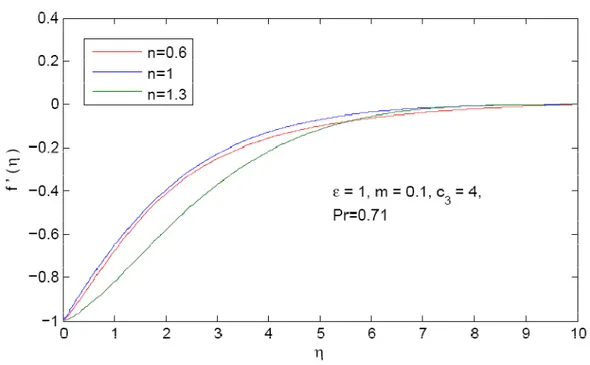
The effects of various parameters for example, the power-law fluid index n, magnetic field number m and the Prandtl number Pr, controlling the parameter b=1,c₁=1 and wall mass transfer c₃ =4 on the velocity f′

( )

η and the temperature field g

( )

η are shown in Figs. 1–8. In Fig. 1 the velocity f '

( )

η is plotted both for both Newtonian

(

n=1

)

and Non-Newtonian (for n=0.6 pseudoplastic and for n=1.3dilatant) fluids in case of linear stretching sheet with m =0 and Pr = 0.71 are fixed. Fig. 2 presents a comparison between hydrodynamic fluid

(

m=0

)

and hydromagnetic (MHD) fluid

(

m≠0

)

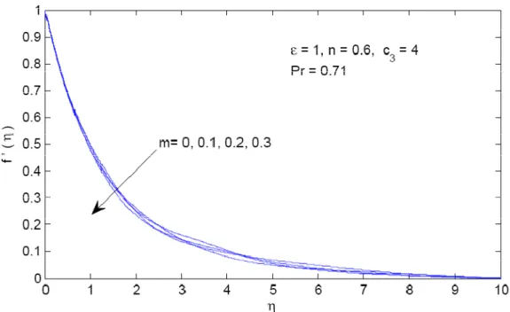
on pseudoplastic fluid in case of linear shrinking sheet for ε = −1,n=0.6, Pr=0.71 and c₃ =4.. Fig. 2 reveals that velocity f '

( )

η

of velocity and boundary layer thickness is observed in case of stretching sheet

(

ε =1

)

for the same fluid as show in Fig. 3. However, this decrement in the velocity of fluid is smaller, as expected in case of stretching sheet than in case of shrinking sheet when compared with hydrodynamic fluid. Fig. 4 depicts the influence of Prandtl number Pr on velocity f '

( )

η of pseudo-plastic fluid

(

n=0.6

)

in presence of magnetic field

(

m=0.1

)

in case of shrinking sheet

(

ε = −1

)

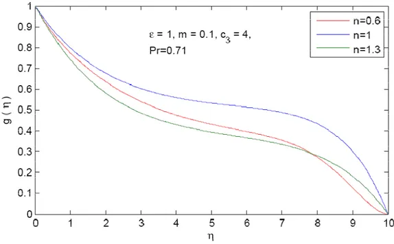
keeping c₄ =4 fixed. It is worth to observe that as Prandtl number increase the velocity of fluid as well the momentum boundary layer thickness decrease. Fig. 5 shows the change in temperature g

( )

η for both Newtonian

(

n=1

)

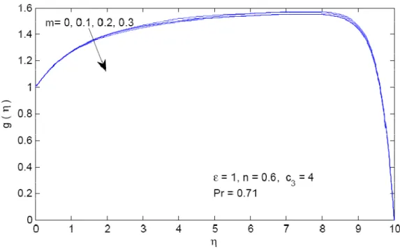
and Non-Newtonian (for n=0.6 pseudoplastic and for n=1.3dilatant) fluids in case of linear stretching sheet with m =0.1 and Pr = 0.71 are fixed. Fig.6 reveals the influence of magnetic field on temperature distribution for pseudo-plastic fluid

(

n=0.6

)

within the domain in case of shrinking sheet with fixed mass transfer and Prandtl’s number. It is evident from this figure that both the temperature and thermal boundary layer thickness decrease by increasing the values of magnetic strength

m. Fig. 7 show that the same trend has been observed for the pseudo-plastic fluid in case of stretching sheet

(

ε =1

)

. However, this decrement in the temperature g

( )

η of pseudo-plastic Non-Newtonian fluid is smaller in case of stretching sheet than in case of shrinking sheet. Fig. 8 shows the change in temperature g

( )

η of Non-Newtonian fluid for different values of Prandtl number Pr by keeping m=0.1,b=1,c₃ =4 fixed over shrinking sheet. It is evident from this figure that both the temperature and thermal boundary layer thickness decrease by increasing the values of Pr. It is also seen that the change in g

( )

η is larger in the case of MHD fluid for larger value of Prandtl number.

6 Concluding

remarks

In this study, Similarity solutions of heat transfer for a MHD viscous power-law fluid over a non-linear porous surface is derived. It is interesting to note that the deductive group theoretic method based on general group of transformation is first time applied to derive proper similarity transformations for the non-linear system of PDEs governing the flow under consideration. The numerical solution for both Newtonian and particular power-law fluid namely pseudo-plastic and dilatant fluid is studied. The influence of pertinent parameters on the physical quantities of interest is reported and discussed. The following conclusions may be extracted from the numerical results:

• For pseudo-plastic fluid the momentum boundary layer thickness decreases by increasing the values of magnetic field m in both cases of shrinking and stretching sheets by controlling flow parameters.

7 Figures

Figure 1: Comparison of the velocity f '

( )

η between Newtonian and Non-Newtonian fluids.

Figure 3: Influence of magnetic field on velocity of dilatant fluid over stretching sheet.

Figure 5: Comparison of temperature g

( )

η for MHD Newtonian and Non-Newtonian fluids.

Figure 7: Effect of magnetic field on temperature of dilatant fluid over stretching sheet.

References

Abbas, Z. and Hayat, T. (2008): Radiation effects on MHD flow in a porous space, Int. J. Heat Mass Transfer , 51, pp. 1024–1033.

Ali, M. E. (1995): On thermal boundary layer on a power law stretched surface with suction or injection, Int. J. Heat Fluid Flow, 16, pp.280-290.

Andersson, H. I. Bech, K. H. and Dandapat, B. S. (1992): Magnetohydrodynamic flow of a power-law fluid over a stretching sheet. Int. J. Non-Linear Mech., 27, pp. 929-936.

Banks, W. H. H. (1983). Similarity solutions of the boundary layer equations for a stretching wall, Journal de Mecanique Theorique et Appliquee, 2, pp. 375-392.

Bataller, R. C. (2008): Similarity solutions for flow and heat transfer of a quiescent fluid over a nonlinearly stretching sheet, J. Mater. Process. Technol., 203, pp. 176–183.

Bluman, J. W. and Kumei, S. (1989): Symmetries and Differential Equations, Springer-Verlag, New York.

Chen, C. K. and Char, M. I. (1988): Heat transfer of a continuous stretching surface with suction or blowing. J. Math. Anal. Appl., 135, pp. 568-580.

Cortell, R. (2005a): A note on magneto hydrodynamic flow of a power law fluid over a stretching sheet. Appl. Math. Comput. 168, pp. 557-566.

Cortell, R. (2007): Viscous flow and heat transfer over a nonlinearly stretching sheet, Appl. Math. Comput., 184, pp. 864–873.

Crane, L. J. (1970): Flow past a stretching plate. ZAMP. 21, pp. 645-647.

Darji, R. M. and Timol, M. G. (2013): Deductive group symmetry analysis for a free convective boundary-layer flow of electrically conducting non-Newtonian fluids over a vertical porous-elastic surface, Int. J. Adv. in Appl. Math. and Mech., 1(1), pp. 1-16.

Datta, B. K., Roy, P. and Gupta, S. (1985): Temperature field in the flow over a stretching sheet with uniform heat flux. Int. Commun. Heat Mass Transfer, 12, pp. 89-94.

Fang, T. (2008): Boundary layer flow over a shrinking sheet with power-law velocity, Int. J. Heat Mass Transfer 51, pp. 5838–5843.

Gupta, P. S. and Gupta, A.S. (1977): Heat and mass transfer on a stretching sheet with suction or blowing. Can. J. Chem. Eng. 55 (6), pp. 744-746.

Ibragimov, N. H. (1985): Transformation Groups Applied to Mathematical Physics, D. Reidel, Dordrecht.

Kalpakides, V. K. (1998): Isovector fields and similarity solutions of nonlinear thermoelasticity. Int. J. Eng. Sci. 36 (10) pp. 1103-1126.

Kalpakides, V. K. (2001): On the symmetries and similarity solutions one-dimensional non-linear thermoelasticity. Int. J. Eng. Sci. 39 (16) pp. 1863-1879.

Koureas, Th., Charalambopoulos, A. and Kalpakides, V. K. (2001): On isovector fields and similarity solutions of generalized dynamic thermoelasticity. Int. J. Eng. Sci. 39 (18), pp. 2071-2087.

Koureas, Th., Charalambopoulos, A. and Kalpakides, V. K. (2003): Symmetry groups and Group-invariant solutions of 3D non-linear thermoelasticity. Int. J. Eng. Sci. 41 (6), pp. 547-568.

Liao, Shi-Jun. (2005): On the analytic solution of magnetohydrodynamic flows of non-Newtonian uids over a stretching sheet. J. Fluid Mech. 488, pp. 189-212.

Lie, S. (1975): Math. Annalen, 8, pp. 220.

Martinson, L. K. and Pavlov, K. B. (1971): Unsteady shear flows of a conducting fluid with a rheological power law. MHD 7, pp. 182-189.

McLeod, J. B. and Rajagopal, K. R. (1987): On the uniqueness of flow of a Navier–Stokes fluid due to a stretching boundary, Arch. Rat. Mech. Anal., 98, pp. 385–393.

Miklavcic, M. and Wang, C. Y. (2006): Viscous flow due to a shrinking sheet, Quart. Appl. Math. 64, pp. 283–290.

Moran, M. J. and Gaggioli, R. A. (1968). Reduction of the number of variables in system of partial differential equations with auxiliary conditions. SIAM J. Appl. Math. 16, pp. 202-215. Morgan A. J. A. (1952): The reduction by one of the number of independent variables in some systems of nonlinear partial differential equations. Quart. J. Math. Oxford 3, pp. 250– 259.

Na, T. Y. (1994): Boundary layer flow of Reiner-Philippoff fluids, lnt. J. Non-Linear Mechanics 29(6), pp. 871-877.

Olver, P. J. (1993): Application of Lie Groups to Differential Equations, Springer-Verlag, 2nd Edition, New York.

Sakiadis, B. C. (1961): Boundary-layer behaviour on continuous solid surfaces, AIChE J., 7, pp. 26-28.

Samokhen, V. N. (1987): On the boundary-layer equation of MHD of dilatant fluid in a transverse magnetic _field. MHD 3, pp. 71-77.

Sarpakaya, T. (1961): Flow of non-Newtonian fluids in a magnetic field. A. I. Ch. E., 7, pp. 324-328.

Suhubi, E. S. (1991): Isovector fields and similarity solutions for general balance equations. Int. J. Eng. Sci. 29 (1), pp. 133-150.

Suhubi, E. S. (1994): Symmetry groups and similarity solutions for radial motions of compressible heterogeneous hyperelastic spheres and cylinders. Int. J. Eng. Sci. 32 (5), pp. 817-837.

Vajravelu, K. (2001): Viscous flow over a nonlinearly stretching sheet, Appl. Math.Comput., 124, pp. 281–288.

Vujanovic B, Stauss A. M. and Djukiv D. J. (1972): A variational solution of the Rayleigh problem for power law non-Newtonian conducting fluid. Ing-Arch. 41, pp. 381-386.