www.atmos-chem-phys.net/16/14853/2016/ doi:10.5194/acp-16-14853-2016
© Author(s) 2016. CC Attribution 3.0 License.
Derivation of the reduced reaction mechanisms of ozone depletion
events in the Arctic spring by using concentration sensitivity
analysis and principal component analysis
Le Cao1, Chenggang Wang1, Mao Mao1, Holger Grosshans2, and Nianwen Cao1 1Key Laboratory for Aerosol-Cloud-Precipitation of China Meteorological Administration, Nanjing University of Information Science and Technology, Nanjing, China
2Institute of Mechanics, Materials and Civil Engineering, Université catholique de Louvain, Louvain-la-Neuve, Belgium
Correspondence to:Le Cao ([email protected])
Received: 13 July 2016 – Published in Atmos. Chem. Phys. Discuss.: 29 August 2016 Revised: 25 October 2016 – Accepted: 5 November 2016 – Published: 1 December 2016
Abstract.The ozone depletion events (ODEs) in the spring-time Arctic have been investigated since the 1980s. It is found that the depletion of ozone is highly associated with an auto-catalytic reaction cycle, which involves mostly the bromine-containing compounds. Moreover, bromide stored in various substrates in the Arctic such as the underlying sur-face covered by ice and snow can be also activated by the absorbed HOBr. Subsequently, this leads to an explosive in-crease of the bromine amount in the troposphere, which is called the “bromine explosion mechanism”.
In the present study, a reaction scheme representing the chemistry of ozone depletion and halogen release is pro-cessed with two different mechanism reduction approaches, namely, the concentration sensitivity analysis and the princi-pal component analysis. In the concentration sensitivity anal-ysis, the interdependence of the mixing ratios of ozone and principal bromine species on the rate of each reaction in the ODE mechanism is identified. Furthermore, the most influ-ential reactions in different time periods of ODEs are also revealed. By removing 11 reactions with the maximum ab-solute values of sensitivities lower than 10 %, a reduced re-action mechanism of ODEs is derived. The onsets of each time period of ODEs in simulations using the original re-action mechanism and the reduced rere-action mechanism are identical while the maximum deviation of the mixing ratio of principal bromine species between different mechanisms is found to be less than 1 %.
By performing the principal component analysis on an array of the sensitivity matrices, the dependence of a
par-ticular species concentration on a combination of the tion rates in the mechanism is revealed. Redundant reac-tions are indicated by principal components corresponding to small eigenvalues and insignificant elements in principal components with large eigenvalues. Through this investiga-tion, aside from the 11 reactions identified as unimportant in the concentration sensitivity analysis, additionally nine reac-tions were indicated to contribute only little to the total re-sponse of the system. Thus, they can be eliminated from the original reaction scheme. The results computed by applying the reduced reaction mechanism derived after the principal component analysis agree well with those by using the orig-inal reaction scheme. The maximum deviation of the mixing ratio of principal bromine species is found to be less than 10 %, which is guaranteed by the selection criterion adopted in the simplification process. Moreover, it is shown in the principal component analysis that O(1D) in the mechanism of ODEs is in quasi-steady state, which enables a following simplification of the reduced reaction mechanism obtained in the present study.
1 Introduction
ppb=parts per billion) to a level lower than 1 ppb within a couple of days. In a following measurement performed at Alert, Canada, not only the occurrence of the ozone deple-tion but also a negative correladeple-tion between the ozone mix-ing ratio and the concentration of filterable bromine (f-Br) was confirmed (Bottenheim et al., 1986; Barrie et al., 1988). Since then, ODEs and the associated bromine enhancement have been reported from various observation sites in polar regions (Kreher et al., 1997; Frieß et al., 2004; Jones et al., 2006, 2009, 2010; Wagner et al., 2007; Helmig et al., 2007, 2012; Halfacre et al., 2014).
Although, the concentration increase of the brominated species was found during ODEs, the mechanism responsible for the destruction of ozone with the involvement of bromine in the troposphere of the Arctic remained a matter of debate until the role of bromine monoxide (BrO) was uncovered by Hausmann and Platt (1994). They suggested that the bromine species participate in an auto-catalytic reaction cycle (R1), namely,
2(Br+O3 →BrO+O2)
BrO+BrO →Br2(or 2 Br)+O2
Br2+hν →2 Br
Net: 2 O3+hν →3 O2
,
(R1) through which the ozone in the boundary layer is consumed without any loss of bromine. In the reaction sequence (R1), BrO participates in self-reactions through which Br atoms are formed. Since the reaction between ozone and Br is rapid, ozone in the boundary layer is continuously consumed in the presence of sunlight via the reaction sequence (R1). How-ever, the reaction cycle (R1) is unable to explain the fast en-hancement of bromine in the ambient air. Therefore, another reaction cycle (R2) is proposed as follows:
Br+O3 →BrO+O2
BrO+HO2 →HOBr+O2
HOBr+H++Br− →mpBr2+H2O
Br2+hν →2 Br
Net: O3+HO2+H++Br−+hν mp
→2 O2+Br+H2O .
(R2) In sequence (R2), the HOBr, which is formed through the ox-idation of BrO, is capable of activating bromide ions stored in various polar substrates such as the suspended aerosols and ice-/snow-covered surfaces. As a result, the bromine amount in the ambient air rises up explosively. This reaction sequence is thus named as “bromine explosion mechanism” (Platt and Janssen, 1995; Platt and Lehrer, 1997; Wennberg, 1999). A detailed review of the auto-catalytic reaction cycles of ODEs and the bromine explosion mechanism is given by Platt and Hönninger (2003), Simpson et al. (2007), and Ab-batt et al. (2012).
Since the 1990s, a large amount of numerical studies on the ozone depletion and halogen release in polar spring have been conducted. At first, zero-dimensional approaches (also
termed “box models”) were employed. Therein, a uniform distribution of the chemical species within the boundary layer was assumed. By using such a model, McConnell et al. (1992) suggested that the heterogeneous reactions that re-lease Br− from the snowpack to the atmosphere are criti-cal for sustaining high levels of BrO and Br in the ambi-ent air. Moreover, Fan and Jacob (1992) showed that the re-lease of Br2from the suspended aerosols is essential for the occurrence of ODEs, whereas Tang and McConnell (1996) and Michalowski et al. (2000) proposed the snowpack above the sea ice surface as a bromine source. The aerosol par-ticles were also included as a source in the photochemi-cal box model MOCCA (Model Of Chemistry in Clouds and Aerosols) by Sander and Crutzen (1996). By adapting MOCCA to polar conditions (Sander et al., 1997), it was found that the rates of reactions between Br and C2H2 or C2H4 are critical for the ozone budget in the troposphere. Later on, the box model MECCA (Module Efficiently Cal-culating the Chemistry of the Atmosphere; Sander et al., 2005, 2006) revealed that the precipitation of CaCO3 from the freezing sea water reduces its buffering ability, which facilitates the acid-catalyzed activation process, as long as the mechanism of evapoconcentration during the formation of aerosol particles is considered (Sander and Morin, 2010). Finally, the authors of this paper (Cao et al., 2014, 2016a) revealed a series of reactions and several initial atmospheric constituents that determine the occurrence of ODEs by per-forming a concentration sensitivity analysis with the box model KINAL (Turányi, 1990a).
representing the vertical mass transfer between layers with different heights to KINAL, and referred to the new model as KINAL-T. Thereby, the influences caused by the change of the boundary layer height on the occurrence and termina-tion of ODEs were studied.
The 3-D model studies on the tropospheric ODEs during polar spring started with Zeng et al. (2003). They suggested, using their regional chemistry transport model, that ODEs persist widespread in a large scale. Afterwards, Yang et al. (2010) added blowing snow as an additional bromine source to the global 3-D tropospheric model p-TOMCAT and found its importance for the bromine explosion. A major advance-ment of the 3-D models was made by Zhao et al. (2008). They used a global 3-D chemistry and transport model GEM-AQ/Arctic to investigate the spatial structure and time se-ries of ozone and BrO in the boundary layer during the Arctic springs of the years 2000 and 2001. The chemistry module MECCA described above was also implemented in GEM-AQ/Arctic, replacing the original chemistry module and solver. It was shown that not only the halogen chem-istry but also the air temperature, atmospheric circulation, and long-range transport of pollutants make great contribu-tions to the springtime ozone depletion in the Arctic. Another version of the 3-D model GEM-AQ incorporating the gas-phase and heterogeneous bromine chemistry was employed by Toyota et al. (2011). They discovered the surface sources of bromine and BrO clouds that were observed in the bound-ary layer of the Arctic (Chance, 1998; Richter et al., 1998; Platt and Wagner, 1998; Wagner et al., 2001). An included source representing the oxidation of Br− by ozone at the snow-/ice-covered surfaces proved later to be the primary source of reactive bromine. In 2013, Cao and Gutheil cou-pled the 3-D model to a LES (large-eddy simulation) of the atmospheric flow using OpenFOAM in order to gain a better understanding of the turbulent mixing of ozone and bromine-related species in the boundary layer during ODEs. In their paper they also discussed the dependence of the ozone de-pletion rate on meteorological conditions such as the wind speed and the boundary layer stability.
The above-discussed theoretical studies revealed that ODEs are influenced by the joint effect of horizontal ad-vection, vertical conad-vection, and local chemistry. The po-tential to provide the information, which may enable in-vestigators to fully understand the underlying physicochem-ical processes, is offered by the numerphysicochem-ical simulation of ODEs of high dimensions with the incorporation of the halo-gen chemistry. However, the possibility of conducting high-dimensional computations of ODEs is usually limited by the effort to calculate the chemical production and destruction source terms in the governing equations. If a complex reac-tion mechanism is adopted in these kinds of simulareac-tions, the execution time for the estimation of chemical source terms can exceed the one for solving transport equations by 1 order of magnitude.
Commonly, a one-step global reaction is adopted in 2-D or 3-D simulations of the atmospheric chemistry that leads to affordable computing times (Warnatz, 1992). However, the coefficients used in the one-step global reaction approach are usually empirical, which cannot be estimated without the aid of experimental studies. An alternative treatment of the chemistry in numerical studies is to choose a couple of el-ementary reactions that are able to describe the important features of the reaction system. However, the selection of el-ementary reactions needs special attention. If the treatment of the chemistry in the computation is too rough and ar-bitrary, the estimation of the chemical production and con-sumption would be inaccurate and, consequently, the simu-lation results may be far from reality. Thus, an appropriate reduced reaction mechanism is required so that the major properties of the original complex reaction mechanism are maintained. Moreover, the size of the reduced reaction mech-anism should be small to enable the efficient computation of high-dimensional equations.
Previously, various approaches have been proposed to sim-plify a complex reaction mechanism while the major prop-erties of the original reaction mechanism are maintained. The first type of the methods is represented by the rate spectrum analysis of the reaction scheme (Turányi et al., 1989). Therein, the rates of competing reactions are pared. However, this method is inapplicable for a very com-plex chemical system in which the influence of each reaction differs significantly on certain kinetic features of the system. The second type of methods is given by the grouping of the reactions into several categories (Edelson and Allara, 1980). The reaction that makes negligible contribution to the flux within its category is considered to be unimportant and, thus, can be eliminated from the reaction scheme. However, the grouping procedure of the reactions depends strongly on the experience of the investigator, which brings some arbitrari-ness to the application of this method. Moreover, the kinetic information inherent in the reaction mechanism may be lost if reactions belonging to a certain chemical kinetic structure are grouped separately. The third type of method is based on the analysis of the production rate of free radicals (Lif-shitz and Frenklach, 1975). Reactions that make small con-tributions to the production or destruction of free radicals are omitted. The fourth approach for obtaining the reduced mechanism is referred to as rate-of-production analysis or reaction-path analysis (Glarborg et al., 1986). Herein, the in-dividual contribution of each reaction to the overall produc-tion rate of selected chemical species is estimated. Moreover, the major formation pathway of the chemical species is iden-tified.
concentrations and the change of reaction rates. Finally, it helps to reduce the size of the reaction mechanism. At present, the sensitivity analysis is often conducted in a “brute force” way (Dodge and Hecht, 1975; Valko and Vajda, 1984) by simply applying a perturbation of reaction rate coeffi-cients by a fixed amount to see the corresponding deviations of particular species concentrations. This is time-consuming and provides only a limited accuracy. Since the 1980s, more systematic and economical approaches for the estimation of the sensitivities have been proposed. The most straightfor-ward one is the concentration sensitivity analysis (Turányi, 1990b), which is capable of displaying the relative impor-tance of an individual rate coefficient on a group of species concentrations and identifying the rate-determining steps in the reaction scheme. The concentration sensitivity analysis has also been used for screening reactions from a compli-cated reaction mechanism in various fields such as the inves-tigation of combustion (Dougherty and Rabitz, 1980; War-natz et al., 2001) and atmospheric chemistry (Turányi and Bérces, 1990).
However, the calculation of the concentration sensitivity coefficients depends on the time interval used in the model, which denotes that the concentration sensitivity is inherently time dependent. Thus, the accuracy of the sensitivity estima-tion is associated with the length of the time interval. Oth-erwise, the concentration sensitivity analysis only discov-ers the importance of an individual input parameter of the chemical kinetic system for several species concentrations while usually the concentrations are influenced by a group of parameters. Thus, another mechanism reduction approach, namely, the principal component analysis, is suggested (Va-jda et al., 1985). The principal component analysis is per-formed based on the calculation of eigenvalues and eigen-vectors of the matrixeSTeS, whereineSdenotes an array of the relative concentration sensitivity matrices. Strongly interact-ing reactions, which significantly influence the concentration of particular species, are identified by principal components with large eigenvalues. Moreover, further mechanistic details of the chemical kinetic system, such as the species in quasi-steady state, can also be provided by the principal component analysis.
Although the mechanism reduction techniques mentioned above have been applied in the investigation of various at-mospheric phenomena, such as the chemistry in clouds (Pan-dis and Seinfeld, 1989), to date little effort has been given to the reduction of the reaction mechanism of ODEs using these techniques. Previous research by the authors (Cao and Gutheil, 2013; Cao et al., 2014) focused on this aspect to some extent. In these studies, relative concentration sensi-tivities of a reaction mechanism of ODEs were computed, and the simplification of the mechanism based on the con-centration sensitivities was prospected. However, the details of the reduction processes were not presented. Furthermore, the reduction technique discussed in these studies (Cao and
Gutheil, 2013; Cao et al., 2014) is only limited to the con-centration sensitivity analysis. Thus, in order to obtain an appropriate reaction mechanism of ODEs with reduced size and adequate accuracy so that the multi-dimensional simula-tions of ODEs are applicable, in the present study, two differ-ent approaches, concdiffer-entration sensitivity analysis and princi-pal component analysis, were applied in a multiphase box model. By doing that, we were able to identify the dominant reactions that govern the bromine chemistry and the ozone depletion during the Arctic spring from the original com-plex reaction mechanism, which in turn saves the computing time in the modeling work of ODEs. The results obtained by using these two mechanism simplification approaches are compared and discussed. The connection between different chemical reactions is also revealed during the reduction pro-cesses.
The manuscript is organized as follows. In Sect. 2, the governing equations of the reduction approaches used in this study are presented. The criteria for screening unimportant reactions from the original reaction scheme are also given in this section. Then the computational results of this work are shown in Sect. 3. Reduced reaction mechanisms derived after the analyses are presented and compared as well. The species in quasi-steady state is also revealed by the implementation of the principal component analysis. Finally, major conclu-sions made in the present study are addressed in Sect. 4. Fur-ther simplification of the reduced reaction mechanism is also prospected.
2 Mathematical model and methods
A complex chemical reaction system can be denoted as dc
dt =f(c,k)+E, (1)
prediction of the temporal change of each chemical species, the choice of this chlorine-free reaction mechanism does not affect the metrics of the present study.
As mentioned above, two different approaches, concentra-tion sensitivity analysis and principal component analysis, are followed to reduce the size of the reaction mechanism of ODEs. The governing equations of these two approaches and the procedures of the mechanism simplification are pre-sented below.
2.1 Concentration sensitivity analysis
The importance of the jth reaction for the ith chemical species is depicted by the relative concentration sensitivity e
Sij, which can be written in the form of e
Sij = ∂lnci ∂lnkj =
kj
ci ∂ci ∂kj =
kj
ci
Sij. (2)
In Eq. (2),ci is the concentration of theith chemical species, andkj denotes the rate coefficient of thejth reaction.Sij= ∂ci/∂kjis the absolute concentration sensitivity, and the unit of Sij depends on the order of thejth reaction. In order to compare the sensitivity coefficients belonging to different re-actions, the normalized version of the sensitivity coefficient, e
Sij, is introduced by multiplyingSijwithkj/ci. The obtained relative concentration sensitivityeSij is thus a dimensionless variable, which represents the percentage of change in the ith species concentration due to a 1 % change of thejth re-action rate constant. The evaluation of the relative concentra-tion sensitivity is helpful for discovering the interdependence between the solution of Eq. (1) and the input parameters such as the reaction rate constantskj.
The calculation ofeSij is performed by differentiating the i-th component of Eq. (1) with respect tokj. With the as-sumption that the local emissions are independent of the rate constants, Eq. (1) becomes
d(∂ci/∂kj)
dt =
ns
X
l=1
∂fi ∂cl
∂cl ∂kj +
∂fi ∂kj
. (3)
The upper limit of the sum in Eq. (3),ns, denotes the total number of the chemical species included in the model. By substituting∂ci/∂kj and∂cl/∂kj in Eq. (3) with the abso-lute concentration sensitivitiesSijandSlj, we obtain another form of Eq. (3) as follows,
dSij dt =
ns
X
l=1
∂fi ∂cl
Slj+ ∂fi ∂kj
. (4)
The second term of the right-hand side of Eq. (4) denotes the direct influence on the concentration change of ith species caused by the perturbation of thejth reaction rate constant. Moreover, as a result of this direct variation in the jth re-action rate, indirect effects on the concentrations of other species are induced via the coupled kinetic system, which
contributes to the solution of Eq. (4). This indirect effect of parameter change is indicated by the first term of the right-hand side of Eq. (4). After obtaining the solutionSij of Eq. (4), the relative concentration sensitivity can be calcu-lated by multiplyingSij withkj/ci. The computation of the absolute concentration sensitivity is conducted by using the subroutine SENS in the chemical kinetic software KINAL (Turányi, 1990a). The decomposed direct method (Valko and Vajda, 1984) is implemented in KINAL for solving Eq. (4), which has been proven to be robust and efficient (Turányi, 1990b).
The concentration sensitivity analysis is a useful measure of how sensitive a specified species concentration is to a par-ticular reaction rate constant. Thus, reactions with large ab-solute values of sensitivities are identified as important and rate-determining. For the purpose of deriving an appropriate reduced reaction mechanism of ODEs, it is necessary to re-move the least important reactions from the original reaction scheme. In the present study, we consider thejth reaction as unimportant if the criterion
max|eSij(t )| ≤10 %;i=1, . . ., ns, t=t (1), . . ., t (nt) (5) is fulfilled. In Eq. (5),ns is the total number of the chemi-cal species as mentioned above, andnt denotes the total time step in the computation. The criterion in Eq. (5) shows that thejth reaction is considered as unimportant if its relative concentration sensitivity for all species at any time point is smaller than 10 % and then can be eliminated from the sys-tem.
reduction approach is chosen, namely, the principal compo-nent analysis, and applied to the original reaction mechanism of ODEs, which is discussed in the section below.
2.2 Principal component analysis
The principal component analysis provides an effective means of screening unimportant reactions from a complex reaction scheme so that a tractable reaction mechanism can be derived. To perform the principal component analysis, we first introduce the normalized rate parameter,α, of which the jth component can be expressed as
αj=lnkj, j=1, . . ., np. (6) Herein,npdenotes the total number of the chemical reactions considered in the model.
The definition given by Eq. (6) enables one to express the response of the reaction mechanism due to a variation in the rate parameters,α, using the response functionQ(α)as fol-lows:
Q(α)=
nt
X
m=1
ns
X
i=1
c
i,m(α)−ci,m(α0)
ci,m(α0) 2
. (7)
In Eq. (7), the subscript “i, m” represents the concentration of ith species at themth time point. ns andnt are the total number of the chemical species and the time step, respec-tively.α0denotes a matrix of the normalized rate parameters with original values.
By applying a Taylor series expansion (Vajda et al., 1985) and a Gauss approximation (Bard, 1974) on Eq. (7), the re-sponse functionQ(α)is approximated as
Q(α)≈Q(eα)=(1α)TeSTeS(1α). (8) Herein, Q(eα)is an approximate response function.1α de-notes a column vector of the parameter perturbations, which has thejth component,
1αj=lnαj−lnαj0. (9) e
Sin Eq. (8) represents an array of the relative concentration sensitivities corresponding to the time instance t (m),m= 1, . . ., nt, and themth element ofeShas the form of
e Sm=
∂lnc1,m
∂lnk1
∂lnc1,m
∂lnk2 . . .
∂lnc1,m
∂lnknp
∂lnc2,m
∂lnk1
∂lnc2,m
∂lnk2 . . .
∂lnc2,m
∂lnknp
..
. ... . .. ... ∂lncns ,m
∂lnk1
∂lncns ,m ∂lnk2 . . .
∂lncns ,m
∂lnknp
. (10) e
S is, thus, a matrix with a dimension of(nt·ns)×np. The eigenvalue–eigenvector decomposition technique is then ap-plied on the matrixeSTeSin Eq. (8), which leads to
e
STeS=U 3UT, (11)
where U is a matrix of normed eigenvectors of eSTeS. 3
represents a diagonal matrix consisting of the eigenvalues λ1, λ2, . . ., λnpofeS
Te
S. By replacingeSTeSin Eq. (8) with the expression shown in Eq. (11), we obtain the approximate re-sponse function in the form of
e
Q(α)=(1α)TU 3UT(1α). (12) We then define the principal component9=UTαin order to writeUT(1α)in the above equation as a variation of the principal component,
19=UT(1α). (13) As a result of the definition of the principal component, Eq. (12) becomes
e
Q(α)=Q(e9)=
np
X
j=1
λjk19jk2, (14)
wherein k19jk2=(19j)T(19j). From Eq. (14), it can be seen that the eigenvalue λj depicts the significance of a group of reactions for the change of the system.19j in Eq. (14) consists ofnpelements, which correspond to closely interacting reactions in the original complex reaction system. It denotes that the species concentrations are influenced not only by a separate individual reaction but also a closely inter-twining reaction sequence. Moreover, the contribution of the individual reaction to its group is also indicated by the weight of the corresponding element in the eigenvectors. Thus, by performing the principal component analysis on the matrix eSTeS, important reactions can be indicated if they correspond to a large element of a principal component associated with a large eigenvalue.
Therefore, after obtaining the relative sensitivity coeffi-cienteSij of the reaction mechanism representing the chem-istry of ODEs, principal component analysis is performed on the matrixeSTeS. In that waynp eigenvalues and the associ-ated eigenvectors are obtained. In order to derive a reaction mechanism with reduced size, we remove the reactions be-longing to the principal components with small eigenvalues. It has been proven in previous studies (Vajda et al., 1985) that if the eigenvalueλj is smaller thanns×nt×10−4, the varia-tion in the concentravaria-tion of each chemical species in the sys-tem is less than 10 % at each instance in time. This selection criterion is also adopted in the present study. Aside from this, in the principal components corresponding to large eigenval-ues, elements with values less than 0.2 are also considered as unimportant and, thus, can be removed from the original mechanism. It was estimated that these elements contribute less than 4 % to the total variation of the concentrations (Va-jda et al., 1985).
Table 1. Initial atmospheric composition in the 200 m boundary layer (ppm is parts per million, ppb is parts per billion, ppt is parts per trillion) (Cao et al., 2014).
Species Mixing ratio
O3 40 ppb
Br2 0.3 ppt
HBr 0.01 ppt
CH4 1.9 ppm
CO2 371 ppm
CO 132 ppb
HCHO 100 ppt
CH3CHO 100 ppt
C2H6 2.5 ppb
C2H4 100 ppt
C2H2 600 ppt
C3H8 1.2 ppb
NO 5 ppt
NO2 10 ppt
H2O 800 ppm
reaction rate constant of the jth reactionkj=0, for which Eq. (6) is invalid. To solve this problem, the parameter e
αj= kj
kj0, j=1, . . ., np (15) is introduced (Vajda et al., 1985). It can be easily deduced thateαj and the parameterαj discussed above yield the same normalized sensitivity eSij. Therefore, the investigation of e
STeSforαj described in the present manuscript is also valid foreαj in the simplification process of the reaction mecha-nism.
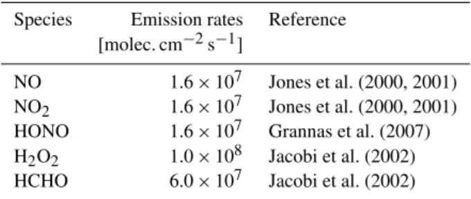
Thus, at first, the original reaction mechanism described above is implemented in the box model KINAL (Turányi, 1990a) to capture the temporal behavior of ozone and prin-cipal bromine species. The boundary layer height used in the model is defined as 200 m. This is considered to be a repre-sentative value since the boundary layer height under typical polar conditions ranges from 100 to 500 m (Stull, 1988). The initial atmospheric composition used in the model is listed in Table 1, taken from the previous box model study (Cao et al., 2014). In the present model, the prescribed 0.3 ppt Br2 and 0.01 ppt HBr play the role of triggering the bromine ex-plosion mechanism and the associated ozone consumption. Emissions of nitrogen oxides (NOx), HONO, H2O2, and HCHO from the underlying surface are also implemented in the model according to the measurements (Jones et al., 2000, 2001; Jacobi et al., 2002; Grannas et al., 2007), and listed in Table 2. The ratio of HONO and NO2is assumed to be in unity (Grannas et al., 2007).
The photolysis frequencies J are evaluated by using a three-coefficient function,
J =J0exp(b[1−sec(cχ )]), (16)
Table 2.Emission fluxes from the underlying surface (Cao et al., 2014).
Species Emission rates Reference
[molec. cm−2s−1]
NO 1.6×10⁷ Jones et al. (2000, 2001)
NO2 1.6×10⁷ Jones et al. (2000, 2001)
HONO 1.6×10⁷ Grannas et al. (2007)
H2O2 1.0×10⁸ Jacobi et al. (2002)
HCHO 6.0×10⁷ Jacobi et al. (2002)
in a three-stream radiation transfer model (Röth, 1992, 2002) with an assumption of SZA (solar zenith angle)=80◦and a surface albedo unity. In Eq. (16),χdenotes the value of SZA. The coefficientsJ0,b, andcare determined in the model by Röth (2002) under the conditions of SZA=0, 60, and 90◦. The values of these parameters, J0, b, and c, used in the present model can be found in our earlier publications (Cao et al., 2014, 2016a). At present, the daily variation in SZA and the dark reactions are not accounted for in the model. The influences brought about by the inclusion of the change in SZA and the dark reactions have been proven to be small in previous investigations (Lehrer et al., 2004; Cao et al., 2014, 2016a).
The heterogeneous reactions representing the bromine re-cycling processes on the surfaces of the ice-/snowpack and the suspended aerosols are also included in the original reac-tion mechanism of ODEs. It has been proven that the rates of these heterogeneous reactions critically control the bromine amount in the boundary layer and the depletion rate of ozone during ODEs (Cao et al., 2014). In the present study, the parameterizations of these heterogeneous reactions are also adopted from the box model study by Cao et al. (2014). For the reactions occurring on or in the suspended aerosols (see Reactions SR14 and SR90 in the Supplement), we adopted a function in the form of Eq. (17) to estimate the reaction rate constantkaerosol:
kaerosol=( r Dg+
4 vthermγ
)−1αeff,aerosol. (17)
the aerosol volume fraction is set equal to 10−5cm3m−3in the present model (Lehrer et al., 2004). With respect to the heterogeneous reactions on the ground surface covered by ice and snow, i.e., Reactions (SR15) and (SR92) in the Supple-ment, the calculation of their rates requires the consideration of the aerodynamic resistance ra, quasi-laminar resistance rb, and surface resistance rc in the model. A typical wind speed observed in the Arctic spring (8 m s−1; Beare et al., 2006) and a roughness length for the ice surface (10−5m; Stull, 1988) are adopted in the estimations of these resis-tances. Moreover, the surface area density of the ground sur-face,αeff,ice=5×10⁻³m−1is obtained with an assumption of a 200 m boundary layer. As a result, the mass transfer coefficientkicefor the heterogeneous Reactions (SR15) and (SR92) is calculated as
kice=(ra+rb+rc)−1αeff,ice. (18) The details of the parameterization of the mass transfer co-efficient are given by Lehrer et al. (2004) and Cao et al. (2014). Recently, a snowpack module representing the mass exchange between the porous snowpack and the ambient air was developed by the author and co-workers (Cao et al., 2016c). However, this snowpack module was not applied in the reaction mechanism used in the present study.
Later, the concentration sensitivity analysis is applied on the original reaction mechanism of ODEs to identify the most influential reactions during different time periods. The tem-poral behavior of the concentration sensitivity coefficient for each reaction is also captured. Then the reactions with a max-imum absolute value of the relative concentration sensitivity less than 10 % are removed from the original reaction scheme so that a reduced reaction mechanism is obtained.
After the computation of the relative concentration sensi-tivity coefficients, the principal component analysis is per-formed on the matrix eSTeS. Principal components corre-sponding to small eigenvalues are regarded as making neg-ligible contributions to the overall response of the whole sys-tem and, thus, can be eliminated. Since 38 chemical species (all species in the mechanism excluding N2) and 94 time steps are focused on in the present simulation, the crite-rion of eigenvalues used for dividing important and unimpor-tant principal components is calculated as 38×94×10−4= 0.3572. Moreover, as discussed above, if an element in a rela-tively important principal component has a value of less than 0.2, this element can be also removed due to its relatively small contribution to the total variation of the system.
In the following section, the most important computational results are presented and discussed.
3 Results and discussion
At the beginning of this study, we ran the box model KI-NAL with the implementation of the original complex re-action scheme to capture the temporal change of principal
Time [days] O3
[p
p
b
]
B
r,
B
rO
,
H
B
r,
H
O
B
r,
B
rtot
[p
p
t]
0 2 4 6 8 10
0 10 20 30 40
0 50 100 150 200
O3 Br BrO HBr HOBr Brtot
Figure 1. Temporal evolution of ozone and principal bromine-containing compounds in a 200 m boundary layer, obtained by using the original reaction scheme in the model (Cao et al., 2016a).
chemical species within the 200 m boundary layer. Figure 1 displays the development of the mixing ratios of ozone and principal bromine species with time. According to previous studies (Cao et al., 2014), the whole ODE can be divided into three periods. In the first period, named “induction stage”, which corresponds to the time period before day 3 in Fig. 1, the consumption rate of ozone in the boundary layer is less than 0.1 ppb h−1. Moreover, the mixing ratio of ozone re-mains steady at a background level (∼40 ppb). Due to the presence of ozone in this time period, the formed Br atoms are rapidly oxidized to be BrO, and thus can be hardly ob-served at this time stage. In contrast to that, the mixing ra-tios of HOBr and BrO steadily increase within this time pe-riod, which makes them the major bromine-containing com-pounds.
After day 3 (see Fig. 1), as bromide is continuously ac-tivated from the ice/snow surface via the bromine explo-sion mechanism, the total bromine loading in the ambient air keeps increasing. As a result, the depletion rate of ozone exceeds 0.1 ppb h−1, and the mixing ratio of ozone declines rapidly until a value lower than 10 % of its original level (4 ppb) is achieved, on approximately day 4.6. This period (from day 3 to day 4.6) is thus named the “depletion stage”. Within the depletion stage, the mixing ratios of BrO and HOBr reach their peaks and then drop instantaneously to a level less than 1 ppt due to the nearly complete removal of ozone in the boundary layer.
Figure 2.
black line in Fig. 1). This large amount of Br is then absorbed by the aldehydes in the atmosphere, and the total bromine amount left in the ambient air becomes steady towards the end of the simulation (see the purple solid line in Fig. 1). Af-ter day 6, the dominant bromine species in the ambient air is mostly in the form of HBr, which is consistent with the previous finding (Langendörfer et al., 1999). The features of the temporal change of these chemical species are similar to those obtained in previous studies (Lehrer et al., 2004; Cao et al., 2014, 2016b, c) except a slight difference in the on-sets of the aforementioned time periods. The discrepancy be-tween the results from different model studies is attributed to the extension of the previous reaction mechanism in the present study.
After capturing the temporal behavior of principal chemi-cal species, the original reaction mechanism consisting of 39 species and 92 reactions is processed with the concentration sensitivity analysis, which is shown in the next subsection.
3.1 Concentration sensitivity analysis of the reaction mechanism of the ODE
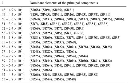
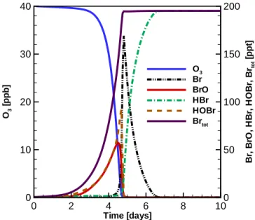
The relative concentration sensitivity coefficient of each chemical species for all the reactions in the original mech-anism within each time step is calculated by performing the concentration sensitivity analysis. Figure 2 depicts the sen-sitivity coefficients of ozone and BrO for all the reactions in the mechanism within the time interval [day 3.9, day 4] which resides within the depletion stage. It can be seen that the sensitivities of the mixing ratios of ozone and BrO to each chemical reaction in the mechanism are clearly indicated by the values of the sensitivity coefficients.
deple-Figure 2.Relative concentration sensitivities of ozone and BrO for(a)Reactions (SR1)–(SR46) and(b)Reactions (SR47)–(SR92) within the time interval [day 3.9, day 4].
tion rate of ozone in this time period. Due to the same reason, reactions with the involvement of HOBr, Reactions (SR10) and (SR11), play significant roles in influencing the mixing ratios of ozone and BrO, which is indicated in Fig. 2a. Aside from the reactions associated with HOBr, reactions which are able to produce or consume Br atoms are also influen-tial since Br reacts with ozone directly and rapidly. Thus, the significance of the Br-associated reactions, Reactions (SR5), (SR7), (SR17), and (SR20), is displayed in Fig. 2a accord-ing to the relatively large absolute values of the sensitivity coefficients. By evaluating the sensitivities at an earlier time instance (not shown here), we found that the Br-associated reactions are the most dominant reactions for ozone and BrO in the induction stage. However, from Fig. 2a, it can be con-cluded that during the depletion stage, the importance of the HOBr-associated reactions exceed the ones with the involve-ment of Br atoms.
In Fig. 2b, it is shown that the nitrogen-related reactions are less important for the mixing ratios of ozone and BrO in the boundary layer compared to the bromine-related
reac-tions. However, the moderate role of the hydrolysis reaction of BrONO2, Reaction (SR90), is depicted. The reason is at-tributable to the formation of HOBr in this reaction, which may also speed up the bromine activation during this time period. Moreover, we found that the reactions with the in-volvement of BrONO2 are of more importance during the end stage, which is consistent with the previous box model study (Cao et al., 2014).
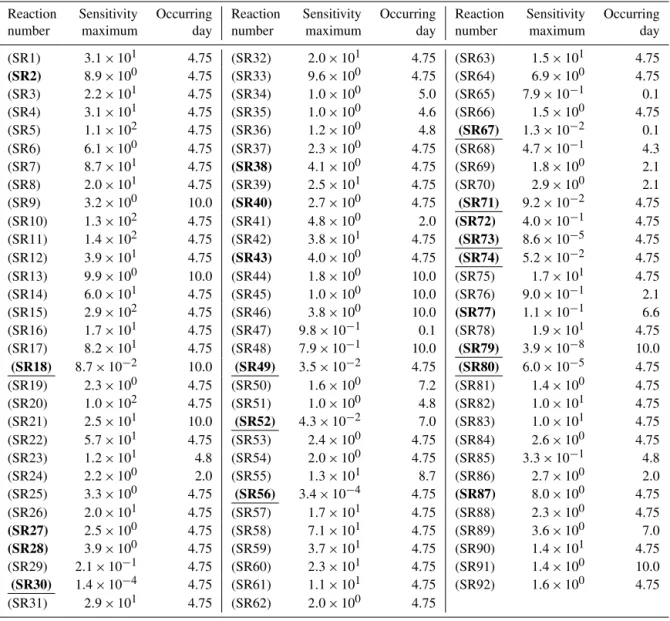
sensitivi-Table 3.The maximum absolute value of the concentration sensitivity coefficient for each reaction in the mechanism and the time when the maximum value occurs. Reaction number underlined denotes that this reaction is identified as unimportant via the concentration sensitivity analysis, and reaction number in bold represents that this reaction is indicated as unimportant via the principal component analysis.
Reaction Sensitivity Occurring Reaction Sensitivity Occurring Reaction Sensitivity Occurring
number maximum day number maximum day number maximum day
(SR1) 3.1×101 4.75 (SR32) 2.0×101 4.75 (SR63) 1.5×101 4.75
(SR2) 8.9×100 4.75 (SR33) 9.6×100 4.75 (SR64) 6.9×100 4.75
(SR3) 2.2×101 4.75 (SR34) 1.0×100 5.0 (SR65) 7.9×10⁻¹ 0.1
(SR4) 3.1×101 4.75 (SR35) 1.0×100 4.6 (SR66) 1.5×100 4.75
(SR5) 1.1×10² 4.75 (SR36) 1.2×100 4.8 (SR67) 1.3×10⁻² 0.1
(SR6) 6.1×100 4.75 (SR37) 2.3×100 4.75 (SR68) 4.7×10⁻¹ 4.3
(SR7) 8.7×101 4.75 (SR38) 4.1×100 4.75 (SR69) 1.8×100 2.1
(SR8) 2.0×101 4.75 (SR39) 2.5×101 4.75 (SR70) 2.9×100 2.1
(SR9) 3.2×100 10.0 (SR40) 2.7×100 4.75 (SR71) 9.2×10⁻² 4.75
(SR10) 1.3×10² 4.75 (SR41) 4.8×100 2.0 (SR72) 4.0×10⁻¹ 4.75
(SR11) 1.4×10² 4.75 (SR42) 3.8×101 4.75 (SR73) 8.6×10⁻⁵ 4.75
(SR12) 3.9×101 4.75 (SR43) 4.0×100 4.75 (SR74) 5.2×10⁻² 4.75
(SR13) 9.9×100 10.0 (SR44) 1.8×100 10.0 (SR75) 1.7×101 4.75
(SR14) 6.0×101 4.75 (SR45) 1.0×100 10.0 (SR76) 9.0×10⁻¹ 2.1
(SR15) 2.9×10² 4.75 (SR46) 3.8×100 10.0 (SR77) 1.1×10⁻¹ 6.6
(SR16) 1.7×101 4.75 (SR47) 9.8×10⁻¹ 0.1 (SR78) 1.9×101 4.75
(SR17) 8.2×101 4.75 (SR48) 7.9×10⁻¹ 10.0 (SR79) 3.9×10⁻⁸ 10.0
(SR18) 8.7×10⁻² 10.0 (SR49) 3.5×10⁻² 4.75 (SR80) 6.0×10⁻⁵ 4.75
(SR19) 2.3×100 4.75 (SR50) 1.6×100 7.2 (SR81) 1.4×100 4.75
(SR20) 1.0×10² 4.75 (SR51) 1.0×100 4.8 (SR82) 1.0×101 4.75
(SR21) 2.5×101 10.0 (SR52) 4.3×10⁻² 7.0 (SR83) 1.0×101 4.75
(SR22) 5.7×101 4.75 (SR53) 2.4×100 4.75 (SR84) 2.6×100 4.75
(SR23) 1.2×101 4.8 (SR54) 2.0×100 4.75 (SR85) 3.3×10⁻¹ 4.8
(SR24) 2.2×100 2.0 (SR55) 1.3×101 8.7 (SR86) 2.7×100 2.0
(SR25) 3.3×100 4.75 (SR56) 3.4×10⁻⁴ 4.75 (SR87) 8.0×100 4.75
(SR26) 2.0×101 4.75 (SR57) 1.7×101 4.75 (SR88) 2.3×100 4.75
(SR27) 2.5×100 4.75 (SR58) 7.1×101 4.75 (SR89) 3.6×100 7.0
(SR28) 3.9×100 4.75 (SR59) 3.7×101 4.75 (SR90) 1.4×101 4.75
(SR29) 2.1×10⁻¹ 4.75 (SR60) 2.3×101 4.75 (SR91) 1.4×100 10.0
(SR30) 1.4×10⁻⁴ 4.75 (SR61) 1.1×101 4.75 (SR92) 1.6×100 4.75
(SR31) 2.9×101 4.75 (SR62) 2.0×100 4.75
ties corresponding to Reactions (SR10), (SR11), and (SR15) are 71, 78, and 164, respectively. The second most important reactions are the Br-associated reactions, Reactions (SR5), (SR7), (SR17), and (SR20) (see Fig. 3). However, the val-ues of their sensitivity coefficients are much lower than those of the HOBr-related reactions during the time period under investigation.
Aiming to reduce the size of the original reaction mech-anism, we summarize the maximum absolute values of the concentration sensitivities for each reaction in the original mechanism (see Table 3). Then the reactions with the max-imum absolute value lower than 10 % are removed from the mechanism. As a result, 11 reactions, namely, Reac-tions (SR18), (SR30), (SR49), (SR52), (SR56), (SR67), (SR71), (SR73), (SR74), (SR79), and (SR80), are eliminated from the original reaction mechanism of ODEs. The reduced
reaction mechanism obtained after the simplification process, thus, contains 39 species and 81 reactions in total.
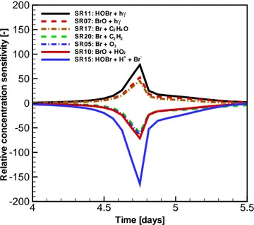
prin-Time [days] R e la ti v e co n c e n tr a ti o n se n s it iv it y [-]
4 4.5 5 5.5
-200 -150 -100 -50 0 50 100 150 200
SR11: HOBr + hγ SR07: BrO + hγ SR17: Br + C H O2 4 SR20: Br + C H2 2 SR05: Br + O3 SR10: BrO + HO2 SR15: HOBr + H + Br+
-Figure 3.Temporal change of the relative concentration sensitivi-ties of ozone for the dominant reactions between day 4 and day 5.5. Here only the reactions with a maximum absolute value of the rela-tive concentration sensitivities larger than 40 are identified as dom-inant and shown.
O3[ppb]
Time [days] B ro m in e -r e la te d s p e c ie s [p p t] O3 [p p b ]
10-3 10-2 10-1 100 101 102
0 2 4 6 8 10 0 50 100 150 200 250 0 10 20 30 40 O3 Brtot Br HOBr BrO HBr
Figure 4.Change of ozone and principal bromine-containing com-pounds plotted with an ozone coordinate axis and a time coordi-nate axis. The solid curves denote the simulation results obtained by using the original reaction mechanism, and the dashed curves represent the results for the reduced reaction mechanism, which is obtained after the concentration sensitivity analysis. The curves of ozone mixing ratios use the axis of time while the principal bromine species correspond to the ozone coordinate axis. Note that the axis of time is in a reverse direction for clarity.
cipal bromine species from these two mechanisms agree very well, within deviations of 1 %.
The principal component analysis was then performed on the sensitivity matrixeSTeSof the original reaction scheme to simplify the mechanism, which is shown in the next subsec-tion.
3.2 Principal component analysis of the reaction mechanism of the ODE
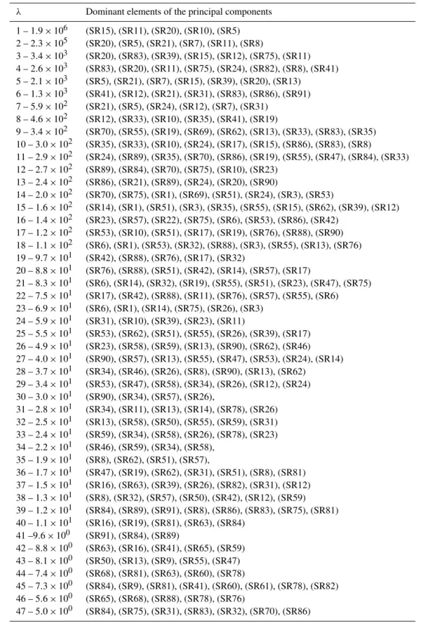
After obtaining the concentration sensitivities of the origi-nal reaction mechanism of the ODE, the matrixeSTeSis con-structed and applied in the principal component analysis. The obtained eigenvalues and the corresponding principal components ofeSTeSare listed in Table 4. The selection cri-terionλi <0.3572 is adopted for removing reactions from the scheme, which has been discussed above. Moreover, in the principal components with large eigenvalues, if an el-ement contributes less than 0.2 to the corresponding prin-cipal component, the reaction associated with this element can be also removed. Thus, by summarizing all the reactions, which are identified as redundant according to the principal component analysis, 20 reactions, Reactions (SR2), (SR18), (SR27), (SR28), (SR30), (SR38), (SR40), (SR43), (SR49), (SR52), (SR56), (SR67), (SR71), (SR72), (SR73), (SR74), (SR77), (SR79), (SR80), and (SR87), can be removed from the original reaction scheme, which are indicated in Table 3 by the reaction numbers in bold.
It is found that the reactions identified as unimportant by using the sensitivity analysis are all covered by the princi-pal component analysis. Moreover, nine extra reactions to be eliminated from the reaction scheme are also revealed by the principal component analysis. The reason for the differ-ence between these two approaches is possibly that in a com-plex reaction mechanism, usually the removal of one single reaction would cause significant variations in the temporal change of many chemical species while the elimination of a group of reactions may have only a minor impact on the response of the system. In the concentration sensitivity anal-ysis, the association between a particular species concentra-tion and each reacconcentra-tion rate is clarified, which is suitable for screening reactions separately. In contrast to that, the princi-pal component analysis is able to identify the dependence of the species concentrations on a group of reactions. There-fore, by performing the principal component analysis, we were able to remove more reactions from the original re-action mechanism. Finally, the reduced rere-action mechanism after the implementation of the principal component analysis consists of 39 species and 72 reactions (see Table 3).
rea-Table 4.Eigenvalues (λ) and the corresponding principal components ofeSTeSfor the original reaction mechanism of the ODE. The first number in the column ofλrefers to the number of the eigenvalue, and the value after the hyphen gives the value ofλ. Here only the principal components with eigenvalues larger than 0.3572 are listed. Within each principal component, elements larger than 0.2 are displayed.
λ Dominant elements of the principal components
1 – 1.9×10⁶ (SR15), (SR11), (SR20), (SR10), (SR5) 2 – 2.3×10⁵ (SR20), (SR5), (SR21), (SR7), (SR11), (SR8)
3 – 3.4×10³ (SR20), (SR83), (SR39), (SR15), (SR12), (SR75), (SR11) 4 – 2.6×10³ (SR83), (SR20), (SR11), (SR75), (SR24), (SR82), (SR8), (SR41) 5 – 2.1×10³ (SR5), (SR21), (SR7), (SR15), (SR39), (SR20), (SR13)
6 – 1.3×10³ (SR41), (SR12), (SR21), (SR31), (SR83), (SR86), (SR91) 7 – 5.9×10² (SR21), (SR5), (SR24), (SR12), (SR7), (SR31)
8 – 4.6×10² (SR12), (SR33), (SR10), (SR35), (SR41), (SR19)
9 – 3.4×10² (SR70), (SR55), (SR19), (SR69), (SR62), (SR13), (SR33), (SR83), (SR35) 10 – 3.0×10² (SR35), (SR33), (SR10), (SR24), (SR17), (SR15), (SR86), (SR83), (SR8)
11 – 2.9×10² (SR24), (SR89), (SR35), (SR70), (SR86), (SR19), (SR55), (SR47), (SR84), (SR33) 12 – 2.7×10² (SR89), (SR84), (SR70), (SR75), (SR10), (SR23)
13 – 2.4×10² (SR86), (SR21), (SR89), (SR24), (SR20), (SR90)
14 – 2.0×10² (SR70), (SR75), (SR1), (SR69), (SR51), (SR24), (SR3), (SR53)
15 – 1.6×10² (SR14), (SR1), (SR51), (SR3), (SR35), (SR55), (SR15), (SR62), (SR39), (SR12) 16 – 1.4×10² (SR23), (SR57), (SR22), (SR75), (SR6), (SR53), (SR86), (SR42)
17 – 1.2×10² (SR53), (SR10), (SR51), (SR17), (SR19), (SR76), (SR88), (SR90) 18 – 1.1×10² (SR6), (SR1), (SR53), (SR32), (SR88), (SR3), (SR55), (SR13), (SR76) 19 – 9.7×101 (SR42), (SR88), (SR76), (SR17), (SR32)
20 – 8.8×101 (SR76), (SR88), (SR51), (SR42), (SR14), (SR57), (SR17)
21 – 8.3×101 (SR6), (SR14), (SR32), (SR19), (SR55), (SR51), (SR23), (SR47), (SR75) 22 – 7.5×101 (SR17), (SR42), (SR88), (SR11), (SR76), (SR57), (SR55), (SR6) 23 – 6.9×101 (SR6), (SR1), (SR14), (SR75), (SR26), (SR3)
24 – 5.9×101 (SR31), (SR10), (SR39), (SR23), (SR11)
25 – 5.5×101 (SR53), (SR62), (SR51), (SR55), (SR26), (SR39), (SR17) 26 – 4.9×101 (SR23), (SR58), (SR59), (SR13), (SR90), (SR62), (SR46) 27 – 4.0×101 (SR90), (SR57), (SR13), (SR55), (SR47), (SR53), (SR24), (SR14) 28 – 3.7×101 (SR34), (SR46), (SR26), (SR8), (SR90), (SR13), (SR62)
29 – 3.4×101 (SR53), (SR47), (SR58), (SR34), (SR26), (SR12), (SR24) 30 – 3.0×101 (SR90), (SR34), (SR57), (SR26),
31 – 2.8×101 (SR34), (SR11), (SR13), (SR14), (SR78), (SR26) 32 – 2.5×101 (SR13), (SR58), (SR50), (SR55), (SR59), (SR31) 33 – 2.4×101 (SR59), (SR34), (SR58), (SR26), (SR78), (SR23) 34 – 2.2×101 (SR46), (SR59), (SR34), (SR58),
35 – 1.9×101 (SR8), (SR62), (SR51), (SR57),
36 – 1.7×101 (SR47), (SR19), (SR62), (SR31), (SR51), (SR8), (SR81) 37 – 1.5×101 (SR16), (SR63), (SR39), (SR26), (SR82), (SR31), (SR12) 38 – 1.3×101 (SR8), (SR32), (SR57), (SR50), (SR42), (SR12), (SR59) 39 – 1.2×101 (SR84), (SR89), (SR91), (SR8), (SR86), (SR83), (SR75), (SR81) 40 – 1.1×101 (SR16), (SR19), (SR81), (SR63), (SR84)
41 –9.6×100 (SR91), (SR84), (SR89)
42 – 8.8×100 (SR63), (SR16), (SR41), (SR65), (SR59) 43 – 8.1×100 (SR50), (SR13), (SR9), (SR55), (SR47) 44 – 7.4×100 (SR68), (SR81), (SR63), (SR60), (SR78)
45 – 7.3×100 (SR84), (SR9), (SR81), (SR41), (SR60), (SR61), (SR78), (SR82) 46 – 5.6×100 (SR65), (SR68), (SR88), (SR78), (SR76)
Table 4.Continued.
λ Dominant elements of the principal components
48 – 4.9×100 (SR68), (SR9), (SR65), (SR81)
49 – 4.3×100 (SR9), (SR65), (SR61), (SR26), (SR63), (SR78), (SR91)
50 – 3.6×100 (SR60), (SR31), (SR84), (SR83), (SR32), (SR82), (SR75), (SR86) 51 – 3.0×100 (SR7), (SR5), (SR61), (SR22), (SR31), (SR81), (SR36)
52 – 2.4×100 (SR69), (SR70), (SR7), (SR60), (SR5) 53 – 1.9×100 (SR22), (SR25), (SR5), (SR7), (SR36)
54 – 1.8×100 (SR81), (SR69), (SR82), (SR7), (SR61), (SR70), (SR63), (SR5) 55 – 1.6×100 (SR36), (SR25), (SR37), (SR69),
56 – 1.5×100 (SR48), (SR64), (SR22), (SR61), (SR78), (SR36), (SR25) 57 – 1.0×100 (SR48), (SR25), (SR22), (SR61),
58 – 9.7×10⁻¹ (SR25), (SR48), (SR64), (SR54), (SR44)
59 – 7.2×10⁻¹ (SR54), (SR44), (SR25), (SR64), (SR66), (SR81), (SR22) 60 – 6.4×10⁻¹ (SR66), (SR64), (SR4), (SR61), (SR78), (SR82), (SR29) 61 – 4.7×10⁻¹ (SR85), (SR66)
62 – 4.3×10⁻¹ (SR66), (SR4), (SR85), (SR76), (SR65), (SR88) 63 – 3.7×10⁻¹ (SR54), (SR44), (SR45), (SR48)
sonably well with those simulated by using the original re-action mechanism. The depletion stage in simulation results using the reduced reaction mechanism starts on day 2.9 and finishes on day 4.4, which occurs a little bit earlier than that using the original reaction mechanism. The maximum devia-tions of Br, HBr, HOBr, BrO, and Brtotare 6.6, 1.6, 8.9, 2.5, and 5.2 %, respectively. Thus, the variations in the mixing ra-tios of the principal bromine species considered in the model caused by the removal of 20 redundant reactions are less than 10 %, which is restrained by the selection criterion adopted. Therefore, the reduced reaction mechanism can satisfactorily capture the temporal change of each chemical species so that the requirement of the accuracy of the reaction mechanism is fulfilled for multi-dimensional computations of ODEs.
The principal component analysis was also applied to dif-ferent time periods of ODEs (induction stage, depletion stage and end stage), and the computational results are displayed in Fig. 6. The yellow contours denote the important re-actions in this time period while the black contours show the reactions that can be removed. Similarly, we summarize all the important reactions at different time stages and move the least significant reactions. It is found that 20 re-actions, Reactions (SR2), (SR18), (SR27), (SR28), (SR29), (SR30), (SR38), (SR40), (SR43), (SR45), (SR49), (SR52), (SR56), (SR67), (SR71), (SR73), (SR74), (SR77), (SR79), and (SR80), can be removed according to the principal com-ponent analysis for different time periods. It should be no-ticed that Reactions (SR29) and (SR45), which are identi-fied as important in the global principal component analysis, are currently indicated as redundant. It is because of that al-though Reactions (SR29) and (SR45) play minor roles and the removal of them causes less than 10 % of the variation in the system response within each time period, from a global
O3[ppb]
Time [days]
B
ro
m
in
e
-r
e
la
te
d
s
p
e
c
ie
s
[p
p
t]
O3
[p
p
b
]
10-3 10-2 10-1 100 101 102
0 2
4 6
8 10
0 50 100 150 200 250
0 10 20 30 40
O3
Brtot Br
HOBr
BrO HBr
Figure 5.Change of ozone and principal bromine-containing com-pounds plotted with an ozone coordinate axis and a time coordi-nate axis. The solid curves denote the simulation results obtained by using the original reaction mechanism, and the dashed curves represent the results for the reduced reaction mechanism, which is obtained after the principal component analysis. The configuration of this figure is similar to that used in Fig. 4.
Figure 6.
Moreover, it is also found that Reactions (SR72) and (SR87), which used to be identified as unimportant, are now considered as important, and cannot be removed from the reaction scheme. From the computational results of the principal component analysis for different time periods (see Fig. 6b), it is observed that Reactions (SR72) and (SR87) are all identified as important in the induction stage while their significance during the depletion stage and the end stage are negligible. Thus, in the principal component analysis when the whole depletion event is observed, the importance of Re-actions (SR72) and (SR87) are smoothed out. As a result, these two reactions can be removed from the original reac-tion scheme.
Apart from screening reactions from a complex reaction mechanism, principal component analysis is also capable to clarify the chemical species in quasi-steady state which are indicated by principal components with small eigenvalues. In order to perform this investigation, the principal compo-nent analysis was once more applied on the reduced reaction mechanism with 39 species and 72 reactions. By observing
the principal components with small eigenvalues (not shown here), we found that no. 71 principal component, which corresponds to the second least eigenvalue, has only two dominant elements, Reaction (SR1): O3+hν→O(1D)+O2 and Reactions (SR3): O(1D)+N2−→O2 O3+N2. Besides, the value of the element (SR1), 0.710, is approximately equal to that of Reaction (SR3), 0.704. We also noticed that Reac-tions (SR1) and (SR3) are the reacReac-tions in which the chemical species O1(D)participates. Thus, it represents that O1(D)is in quasi-steady state, and the computational results depend only on the ratio of the reaction rates of Reactions (SR1) and (SR3), which can be expressed as
ks= k1 k3
. (19)
Figure 6.The importance of each reaction in the original reaction mechanism within different time periods, for(a)Reactions (SR1)–(SR46) and (b)Reactions (SR47)–(SR92). Yellow contour denotes that this reaction is important through this time period, while black contour represents that this reaction is identified as insignificant during this time stage.
principal bromine species calculated from the reduced reac-tion mechanism and from the reacreac-tion scheme with the mod-ified reaction rates agree well within 1 %. In contrast to that, if we only increase the rate constant of Reaction (SR1) to 100 times of its original value while the rate constant of Re-action (SR3) remains the same, the difference between the results from the original mechanism and the modified mech-anism becomes larger (see Table 5). The maximum deviation amounts to 172 % for the species HOBr. This finding also confirms the validity of the principal component analysis.
As O1(D)was found in quasi-steady state during ODEs, it is possible to directly estimate the mixing ratio of O1(D) at each time instance according to the mixing ratios of other chemical species. It can be easily deduced that the mixing ratio of O1(D)during the depletion event can be expressed as
[O1(D)] =k1[O3] k3[N2]
, (20)
Table 5. Comparison of the peak values of principal bromine species calculated by using various chemical reaction mechanisms. The peak values shown in the table are calculated by using the re-duced reaction mechanism derived after the principal component analysis.
Species Peak value k1×100,k3×100 k1×100,k3×1
[ppt] deviation [%] deviation [%]
Br 177.6 0.3 104.4
HBr 203.7 0.1 126.8
HOBr 95.6 0.7 172.0
BrO 58.1 0.1 63.7
Brtot 203.8 0.1 126.7
to shorten the time cost for the calculation of the chemical source terms, the species equation corresponding to O1(D) can be also simplified, which improves the efficiency of the computations. However, the simplification of the reaction mechanism by using the quasi-steady-state approximation is beyond the scope of the present study.
4 Conclusions and future developments
In the present study, two reduction approaches, namely, the concentration sensitivity analysis and the principal compo-nent analysis, were applied on a reaction mechanism repre-senting the chemistry of ODEs. The former was performed based on the ratio of the relative change of species concentra-tions and the variation of a particular reaction rate. The sig-nificance of each reaction in the original mechanism for var-ious chemical species was identified. It was found that dur-ing the depletion of ozone, reactions associated with HOBr are the most influential reactions as they determine the total bromine loading in the atmosphere within this time period. By removing 11 reactions, which exhibit peak absolute val-ues of the sensitivity coefficients lower than 10 %, a reduced reaction mechanism of ODEs was derived. The difference between the results obtained by using the original reaction mechanism and the reduced reaction mechanism is negligi-ble, which validates the sensitivity analysis.
The principal component analysis, on the other hand, is able to extract inherent information from a chemical kinetic system via the eigenvalue decomposition of the matrixeSTeS. In the herein presented study, the reactions that have princi-pal components with eigenvalues lower than a critical crite-rion were eliminated from the original reaction mechanism. Additionally, the elements that occupy less than 0.2 of each principal component were also removed. In total, 20 reac-tions were identified as redundant using the principal compo-nent analysis and, thus, screened out from the original ODE mechanism. As a result, a reaction scheme with a reduced size consisting of 39 species and 72 reactions was obtained. The deviations of the mixing ratios of ozone and principal bromine species between the original reaction mechanism and the reduced reaction mechanism after the principal com-ponent analysis are within 10 %. This proves the suitabil-ity of the obtained reduced reaction mechanism for multi-dimensional simulations of ODEs. Apart from this, displayed by the principal components with the smallest eigenvalues, the chemical species O1(D)is identified to be in quasi-steady state. This facilitates a further improvement of the numerical efficiency in high-dimensional simulations of ODEs.
It should be noted that the horizontal advection, which makes a contribution to the occurrence and termination of ODEs, cannot be captured by the present box model due to the inherent limitations of the 0-D model. In earlier stud-ies, by investigating the origin of the ozone-depleted air at three observational sites in the springtime Arctic,
Botten-heim and Chan (2006) revealed that the occurrence of ODEs is linked to a several-day horizontal transport of the cold, ozone-depleted air across the Arctic Ocean covered with fresh sea ice. Their conclusion is also supported by the sta-tistical analysis performed by Hirdman et al. (2009). More-over, Toyota et al. (2011) found in their 3-D model study that the termination of ODEs during the Arctic spring is associated with enhanced boundary-layer wind transported from the south, carrying the ozone-rich air to the location under observation. However, by showing the dependency of the hourly mean ozone level on the wind speed at Barrow, Alaska, during the springtime of 2009, Helmig et al. (2012) suggested that ODEs are more frequently observed under a calm-wind condition (wind speed<5 m s−1). Thus, the rela-tive importance of the horizontal advection for ODEs is still under debate. In order to clarify this, a fully coupled 3-D model is needed, which is beyond the scope of the present box model study. For a future development of the model used in this study, the advection process can be parameterized as a reaction sequence in the mechanism. After this parameteriza-tion, it is possible to implement the simplification approaches presented in this study on the reaction mechanism with the inclusion of the horizontal advection.
from the kinetic reaction scheme. Apart from this, currently, another type of a timescale-based analysis approach, the in-trinsic low-dimensional manifolds (ILDM) (Maas and Pope, 1992), is being implemented by the authors of this paper. By means of the ILDM, the dimension of the composition space can be reduced significantly based on the number of the freedom degrees. As a result, the computational effort of the chemical source terms in the rate equations is decreased remarkably, which may further progress the current work.
5 Data availability
The output data of the model for the sensitivity analysis and the principal component analysis are available upon request to the contact author Le Cao ([email protected]).
The Supplement related to this article is available online at doi:10.5194/acp-16-14853-2016-supplement.
Acknowledgements. The authors are sincerely thankful for the financial supports provided by the National Natural Science Foun-dation of China (no. 41375044), the Natural Science FounFoun-dation of Jiangsu Province (no. 2015s042), the Double Innovation Talent Program (no. R2015SCB02), the Polar Strategic Foundation (no. 20150308), and the Startup Foundation for Introducing Talent of NUIST (no. 2014r066). We also like to thank two anonymous reviewers and the editor Marc von Hobe for their perspicacious comments that significantly improved our work.
Edited by: M. von Hobe
Reviewed by: two anonymous referees
References
Abbatt, J. P. D., Thomas, J. L., Abrahamsson, K., Boxe, C., Gran-fors, A., Jones, A. E., King, M. D., Saiz-Lopez, A., Shep-son, P. B., Sodeau, J., Toohey, D. W., Toubin, C., von Glasow, R., Wren, S. N., and Yang, X.: Halogen activation via interac-tions with environmental ice and snow in the polar lower tropo-sphere and other regions, Atmos. Chem. Phys., 12, 6237–6271, doi:10.5194/acp-12-6237-2012, 2012.
Atkinson, R., Baulch, D. L., Cox, R. A., Crowley, J. N., Hampson, R. F., Hynes, R. G., Jenkin, M. E., Kerr, J. A., Rossi, M., and Troe, J.: Summary of evaluated kinetic and photochemical data for atmospheric chemistry, IUPAC Subcommittee on Gas Kinetic Data Evaluation for Atmospheric Chemistry, Cambridge, UK, available at: http://www.iupac-kinetic.ch.cam.ac.uk/ (last access: 26 November 2016), 2006.
Bard, Y.: Nonlinear parameter estimation, Academic Press, New York, 1974.
Barrie, L. A., Bottenheim, J. W., Schnell, R. C., Crutzen, P. J., and Rasmussen, R. A.: Ozone destruction and photochemical reac-tions at polar sunrise in the lower Arctic atmosphere, Nature, 334, 138–141, doi:10.1038/334138a0, 1988.
Beare, R., Macvean, M., Holtslag, A., Cuxart, J., Esau, I., Golaz, J.-C., Jimenez, M., Khairoutdinov, M., Kosovic, B., Lewellen, D., Lund, T., Lundquist, J., Mccabe, A., Moene, A., Noh, Y., Raasch, S., and Sullivan, P.: An intercomparison of large-eddy simulations of the stable boundary layer, Bound.-Lay. Meteorol., 118, 247–272, doi:10.1007/s10546-004-2820-6, 2006.
Bott, A.: A numerical model of the cloud-topped planetary boundary-layer: Impact of aerosol particles on the radiative forc-ing of stratiform clouds, Q. J. Roy. Meteor. Soc., 123, 631–656, doi:10.1002/qj.49712353906, 1997.
Bott, A.: A flux method for the numerical solution of the stochas-tic collection equation: extension to two-dimensional parstochas-ticle distributions, J. Atmos. Sci., 57, 284–294, doi:10.1175/1520-0469(2000)057<0284:AFMFTN>2.0.CO;2, 2000.
Bott, A., Trautmann, T., and Zdunkowski, W.: A numerical model of the cloud-topped planetary boundary-layer: Radiation, turbu-lence and spectral microphysics in marine stratus, Q. J. Roy. Me-teor. Soc., 122, 635–667, doi:10.1002/qj.49712253105, 1996. Bottenheim, J., Gallant, A., and Brice, K.: Measurements of NOy
species and O3at 82◦N latitude, Geophys. Res. Lett., 13, 113– 116, doi:10.1029/GL013i002p00113, 1986.
Bottenheim, J. W. and Chan, E.: A trajectory study into the origin of spring time Arctic boundary layer ozone depletion, J. Geophys. Res.-Atmos., 111, D19301, doi:10.1029/2006JD007055, 2006. Cao, L. and Gutheil, E.: Numerical simulation of tropospheric
ozone depletion in the polar spring, Air Qual. Atmos. Health, 6, 673–686, doi:10.1007/s11869-013-0208-9, 2013.
Cao, L., Sihler, H., Platt, U., and Gutheil, E.: Numerical analysis of the chemical kinetic mechanisms of ozone depletion and halogen release in the polar troposphere, Atmos. Chem. Phys., 14, 3771– 3787, doi:10.5194/acp-14-3771-2014, 2014.
Cao, L., He, M., Jiang, H., Grosshans, H., and Cao, N.: Sensitivity of the reaction mechanism of the ozone depletion events during the Arctic spring on the initial atmospheric composition of the troposphere, Atmosphere, 7, 124, doi:10.3390/atmos7100124, 2016a.
Cao, L., Platt, U., and Gutheil, E.: Role of the boundary layer in the occurrence and termination of the tropospheric ozone de-pletion events in polar spring, Atmos. Environ., 132, 98–110, doi:10.1016/j.atmosenv.2016.02.034, 2016b.
Cao, L., Platt, U., Wang, C., Cao, N., and Qin, Q.: Numeri-cal Analysis of the Role of Snowpack in the Ozone Depletion Events during the Arctic Spring, Atmos. Chem. Phys. Discuss., doi:10.5194/acp-2016-553, in review, 2016c.
Chance, K.: Analysis of BrO measurements from the Global Ozone Monitoring Experiment, Geophys. Res. Lett., 25, 3335–3338, doi:10.1029/98GL52359, 1998.
Dodge, M. and Hecht, T.: Rate constant measurements needed to improve a general kinetic mechanism for photochemical smog, Int. J. Chem. Kinet., 7, 155–163, 1975.
Dougherty, E. P. and Rabitz, H.: Computational kinetics and sensi-tivity analysis of hydrogen-oxygen combustion, J. Chem. Phys., 72, 6571–6586, 1980.
![Figure 2. Relative concentration sensitivities of ozone and BrO for (a) Reactions (SR1)–(SR46) and (b) Reactions (SR47)–(SR92) within the time interval [day 3.9, day 4].](https://thumb-eu.123doks.com/thumbv2/123dok_br/18253900.342607/10.918.180.746.95.650/figure-relative-concentration-sensitivities-ozone-reactions-reactions-interval.webp)