© 2005 Author(s). This work is licensed under a Creative Commons License.
Nonlinear dynamics of turbulent waves in fluids and plasmas
K. He1and A. C.-L. Chian2
1Inst. of Low Ener. Nucl. Phys., Beijing Normal Univ., Beijing, 100875 China
2National Institute for Space Research (INPE), P.O. Box 515,12227-010, S˜ao Jos´e dos Campus-SP, Brazil
Received: 14 September 2004 – Revised: 23 November – Accepted: 15 December 2004 – Published: 4 January 2005 Part of Special Issue “Nonlinear processes in solar-terrestrial physics and dynamics of Earth-Ocean-System”
Abstract. In a model drift wave system that is interesting both in fluids and plasmas, we find that an embedded mov-ing saddle point plays an important role at the onset of turbu-lence. Here the saddle point is actually a saddle steady wave, in its moving frame the wave system can be transformed into a set of coupled oscillators whose motion is affected by the saddle steady wave as if it is a potential. It is found that a collision with the saddle point triggers a crisis, following the collision another dynamic event occurs which involves a transition in the phase state of the master oscillator. Only after the latter event the spatial regularity is destroyed. The phase dynamics before and after the transition is further in-vestigated. It is found that in a spatially coherent state before the transition the oscillators reach a functional phase syn-chronization collectively with or without phase slips, after the transition in the turbulent state an on-off imperfect syn-chronization is established among the oscillators with long wavelengths. When the synchronization is on, their ampli-tudes grow up simultaneously, giving rise to a burst in the total wave energy. A power law behavior is observed in the correlation function between phases of the oscillators. Poten-tial application of our results in prediction of energy bursts in turbulence is discussed.
1 Introduction
Turbulence can be observed in systems of very different in scales and properties, which is an important topic in a variety of disciplines (Frisch, 1995). In the sun and other stars, flares and electromagnetic emissions are observed, it has been sug-gested that, e.g. solar flares are caused by nonlinear dynamics of solar plasma turbulence (Boffetta et al., 1999). In our en-vironment, e.g. in space, oceans and atmosphere, turbulence is often encountered, which impact on human lives for thou-sands of years. In biological systems turbulence may play an
Correspondence to:K. He
active role, e.g. brain dynamics is turbulent when it is awake (Kandel et al., 2000).
In contrast to wide awareness of turbulence, people knew little about its mechanism until recently when great progress has been made in the investigation of nonlinear dynamics. A great deal of experimental evidence has been found that strengthens the confidence that turbulence can be understood on the basis of nonlinear dynamics. Some scenarios to chaos, e.g. period-doubling, Ruelle-Takens route as well as inter-mittency, have found supports from experimental and theo-retical investigations (Lichtenberg and Lieberman, 1983; In-feld and Rowlands, 1990; Eckmann, 1981; Swinney, 1983; Biskamp and He, 1985; Klinger et al., 1997). This progress encourages scientists to further study turbulence in spatially extended systems. In this area abundant phenomena, such as various space-time patterns, solitons, weak and strong tur-bulence are not yet fully understood and worthwhile to be explored (Cross and Hohenberg, 1993; Bishop et al., 1983; Chat´e and Manneville, 1987; He and Salat, 1989; Chian et al., 2002). In this paper we will present some results of our investigation on dynamics of nonlinear waves, the attention will be focused on the questions as what causes a spatially regular wave to transit to a spatiotemporal chaotic wave or a turbulence. In our discussion effect of a saddle point and phase dynamics will be emphasized.
regimes where hystereses exist (He and Salat, 1989). An-other significant phenomenon is: when its wave energy is in the negative tangential branch of an S-shaped hysteresis a steady wave solution is unstable due to a saddle-node in-stability. Such a saddle steady wave can not be realized, it is a virtual wave embedded in certain realized waves, e.g. in some stable solitary waves, or in periodic, chaotic and turbu-lent waves. These phenomena lead to our conjecture that an embedded saddle steady wave may play an important role at the onset of turbulence.
In general, a steady wave solution is like a solitary wave, which moves in a constant group velocity with an invariable shape. If observed in the reference frame moving with this group velocity, a steady wave solution is a fixed point in the Fourier space. With variation of applied parameters such a fixed point may lose its stability, just like what happens in time-dependent systems. If the instability is of saddle type, this steady wave solution is a saddle point. Therefore, in a reference frame moving with its group velocity, a saddle steady wave solution is an embedded saddle point, in another word, in the lab frame it is a moving saddle point embedded in the realized wave.
Indeed we have found convincing evidence in the driven/damped drift-waves that such an embedded saddle point plays a critical role at the onset of turbulence. We find that a collision with the saddle point triggers a crisis. How-ever, this collision does not directly destroy the spatial coher-ence. Then a further question is: how the spatial coherence is destroyed? To answer this question the motion of different spatial scales has to be studied. To this end we transform the wave system to a set of coupled oscillators moving in a po-tential of the saddle steady wave solution, and find that sub-sequently to the collision there occurs another critical event during which the phase of the master oscillator experiences a trapped-free transition. It is this event that plays a key role in the destruction of spatial coherence. These results will be given in Sect. 2. In the following sections we investigate the dynamics of the oscillators, especially of their phases. We find that, in spatially regular wave before the transition per-fect functional relations are formed between the mode phases (ref. Sect. 3), in a turbulent wave after the transition the os-cillators show much stronger tendency to establish a phase synchronization (PS), however, due to the embedded saddle point they are not easy to reach a perfect PS, instead, an on-off imperfect PS is established among the oscillators (ref. Sect. 4). At “on” stages of the synchronization amplitudes of the oscillators of different scales grow up almost simulta-neously, inducing bursts in the total wave energy. This re-sult presents an explanation for the dynamic cause of energy bursts in the turbulent motion. Finally Sect. 5 is a conclusion and discussion.
2 Crisis-induced transition to spatiotemporal chaos
In He (1998) we found a crisis-induced transition from a spa-tially regular to spatiotemporally chaotic wave in the
follow-ing model equation, ∂φ
∂t +a ∂3φ ∂t ∂x2+c
∂φ ∂x +f φ
∂φ
∂x = −γ φ−εsin(x−t ).(1) Without drivingεand dampingγ the system describes shal-low water wave in fluids (Dodd et al., 1982; Benjamin et al., 1972) and drift wave in magnetized plasmas (Horton, 1990), so Eq. (1) has practical applications.
A steady wave solution of Eq. (1) has a form ofφ0(x−t ),
which is a fixed point in the reference frameξ=x−t,τ=t. Hereφ0(ξ )obeys a steady equation,
∂φ0
∂τ =0. (2)
By expanding φ0(ξ )=PkAkcos(kξ+θk) (here and in the following k=1,2,· · ·, N→∞) and with appropriate guessed values one can work out its mode amplitudes and phases, {Ak, θk}, thenφ0(ξ ) is obtained. Its wave energy,
E0≡E(φ=φ0), is a constant, here
E(t )= 1 2π
Z 2π
0
1 2[φ
2(t )−aφ2
x(t )]dx. (3) It has been found that for givenin certain regimes steady wave energy E0 as a function of ε forms an S-hysteresis.
Stability analysis shows that when its energy locates in the negative tangential branch of a hysteresis a steady wave so-lutionφ0is unstable due to a saddle-node instability, such a
saddle steady wave is denoted asφ0∗(ξ )in the following, in the (ξ,τ) frame it is a saddle point in the Fourier space. In the following we will see that this saddle point plays a critical role in the transition to turbulence. On the other hand, if its wave energy locates in the lower branch of a S-hysteresis a steady wave solutionφ0(x−t )can be stable, or it may lose
the stability through a Hopf bifurcation (He , 2004).
To study the complicated dynamic behaviors we have used the pseudospectral method to solve Eq. (1) in periodic bound-ary condition, φ (x+2π )=φ (x). In the chosen parameter regimes 26 to 29 spatial grids are tested, the results are in
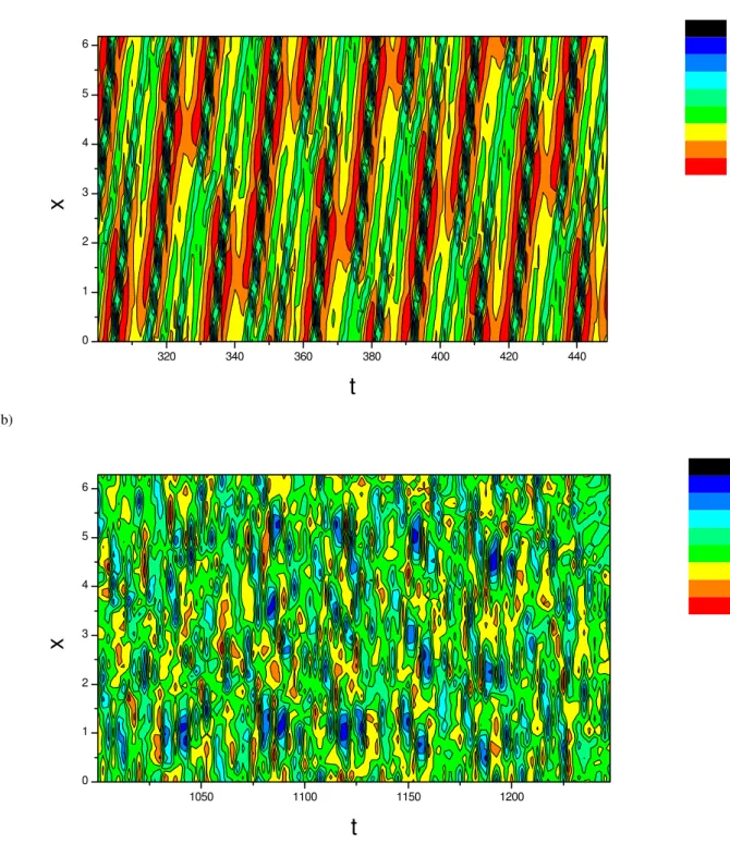
agreement with each other. Among others, we found that for a givenin certain regime there exists a criticalε=εc, be-fore which the wave is spatially regular although it can be erratic in time, but after which spatial regularity of the wave is destroyed, the wave looks very turbulent, in particular it bears some characteristic feature of fully-developed turbu-lence, e.g. a power law spatial spectrum. For=0.65 the critical transition pointεc≈0.20. Figure 1 shows the typical space-time contour plot of (a) spatially regular wave where one can still see a wave structure and (b) spatiotemporally chaotic wave where the wave is broken.
320 340 360 380 400 420 440 0
1 2 3 4 5 6
t
x
-0.8000 -0.6500 -0.5000 -0.3500 -0.2000 -0.05000 0.1000 0.2500 0.4000
(b)
1050 1100 1150 1200
0 1 2 3 4 5 6
t
x
-1.400 -1.075 -0.7500 -0.4250 -0.1000 0.2250 0.5500 0.8750 1.200
Fig. 1.Space-time contour plot ofφ (x, t )for(a)spatially regular wave before the transition withε=0.19,(b)spatiotemporally chaotic wave after the transition withε=0.22;=0.65.
when the realized waveφ (x, t ) evolves to about the same shape of saddle steady wave φ0∗(x−t ) (He, 2000). Fig-ure 2 shows a contour plot of12(x, t )for=0.65, ε=0.22, here1(x, t )≡|φ (x, t )−φ0∗(x−t )|is the space-time differ-ence between the realized wave and saddle steady wave. In this example whent <∼30 the realized waveφ (x, t )is spa-tially regular, whent >∼50 it transits to a state of extreme irregularity both in time and in space. In the plot one can
0 50 100 150 200 0
1 2 3 4 5 6
t
x
0 0.03750 0.07500 0.1125 0.1500 0.2250 0.3000 0.6000 0.9000 1.200 1.500 1.800 2.100 2.400
Fig. 2. Contour plot of space-time distance between the realized wave and the saddle steady wave,12(x, t )≡|φ (x, t )−φ∗0(x−t )|2,
=0.65,ε=0.22.
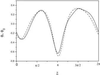
this solution exists only theoretically; however, just att≈t∗ the saddle steady waveφ0∗(x−t∗)appears approximately in reality, in this case a disturbance to it would grow along its unstable orbit, a crisis then sets in which finally leads to the spatiotemporal chaotic attractor.
Since a saddle steady wave is a saddle point in the (ξ,τ) frame, we anticipate that a collision with the saddle point can be observed at onset of the crisis(Ott, 1993). With this con-sideration at first we project the orbit onto a Poincar´e section, the one that was used in He (1998), unfortunately in this rep-resentation we failed to see such a collision, an apparent gap always shows up between the realized orbit and the saddle point at the onset of crisis. Later on, we realized the reason why the collision can not be manifested in a Poincar´e section: although at the critical timet∗ the realized wave φ (x, t∗) evolves to a shape very similar to that of the virtual wave φ0∗(x−t∗), the two waveforms are never exactly the same (see Fig. 3), in particular the discrepancy between their high kmodes can be apparent. In fact, a representation in which the collision can be observed should be in accordance with what happens at the onset of crisis, that is, in accordance with the phenomenon of “pattern resonance”. With this in mind we choose a representation∂φ (ξ=0, τ )/∂ξvs.φ (ξ=0, τ )in which such a collision can be fairly well demonstrated (He and Chian, 2004).
Instead of pseudospectral method applied to obtain Figs. 1, 2 and 3, for demonstrating the collision and other mecha-nisms we prefer to use a different approach. Since in (ξ,τ) frame a steady wave solutionφ0(ξ )is a fixed point, it allows
us to setφ (ξ, τ )=φ0(ξ )+δφ(ξ,τ), then from Eq. (1) the
ac-tive part of the wave,δφ(ξ,τ), is governed by the following equation,
∂ ∂τ[1+a
∂2
∂ξ2]δφ−
∂ ∂ξ[1+a
∂2
∂ξ2]δφ+c
∂ ∂ξδφ +γ δφ+f ∂
∂ξ[φ0(ξ )δφ] +f δφ ∂
∂ξδφ=0. (4)
-0.8 -0.6 -0.4 -0.2 0.0 0.2 0.4
3π/2
π/2 π 2π
0
φ
,
φ 0
ξ
Fig. 3. Waveforms of the realized waveφ (x, t∗)(solid line) and the virtual saddle steady waveφ∗0(x−t∗)(dashed line) at the critical time of ‘pattern resonance’,t∗≈39.0, the same case as in Fig. 2.
Substituting the expansion of φ0(ξ ) as well as δφ (ξ,
τ )=Pkbk(τ )cos[kξ+αk(τ )]into Eq. (4) we obtain a set of ordinary differential equations for the modes{bk(τ ), αk(τ )} ofδφ (ξ, τ ):
dbk dτ = −
γ
1−ak2bk+
f k 2(1−ak2)
×{ X i+j=k
[Aibjsin(θi+αj−αk)+bibjsin(αi+αj−αk)/2]
+ X
i−j=k
[Aibjsin(θi−αj−αk)+bibjsin(αi−αj−αk)/2] X
j−i=k
[Aibjsin(−θi+αj−αk)+bibjsin(−αi+αj−αk)/2]},
dαk dτ = −k[
c
1−ak2 −] −
f k 2(1−ak2)b
k
×{ X i+j=k
[Aibjcos(θi+αj−αk)+bibjcos(αi+αj−αk)/2]
+ X
i−j=k
[Aibjcos(θi−αj−αk)+bibjcos(αi−αj−αk)/2]
+ X
j−i=k
[Aibjcos(−θi+αj−αk)+bibjcos(−αi+αj−αk)/2]}. (5) Owing to the last term in the left hand side of Eq. (4), modes bk(τ )andαk(τ )of different wavenumberkare coupled with each other; besides, their motion is also affected by the steady wave solutionφ0(ξ )as if the latter is a potential well.
Therefore, with Eqs. (5) we have transformed the nonlinear wave Eq. (1) into a set of coupled oscillators{bk(τ ),αk(τ )} in a potentialφ0(ξ ). After the modes ofφ0(ξ ), i.e.{Ak, θk}, are obtained, temporal variations of{bk(τ ),αk(τ )}and hence δφ(ξ,τ) can be worked out. Sinceφ0(ξ )is a solitary
-0.6 -0.4 -0.2 0.0 0.2 -2
-1 0 1
-0.6 -0.4 -0.2 0.0 0.2
-2 -1 0 1
-0.6 -0.4 -0.2 0.0 0.2
-2 -1 0 1
-0.4 0.0 0.4 0.8
-4 -2 0 2
(a)
ε=0.18
d
φ
/d
ξ
(
ξ
=0)
(c)
ε=0.2009
(b)
ε=0.19
d
φ
/d
ξ
(
ξ
=0)
φ
(
ξ=0)
(d)
ε=0.201
φ
(
ξ=0)
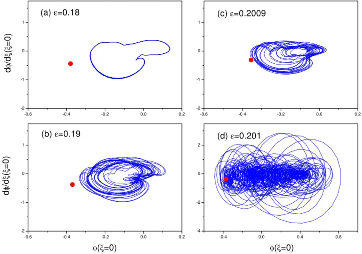
Fig. 4. Asymptotic attractor ofφ (ξ, τ )(solid line) and saddle point ofφ0∗(ξ )(bullet) in phase space∂φ (0, τ )/∂ξ vs.φ (0, τ )for=0.65 with(a)ε=0.18,(b)0.19,(c)0.2009 before the crisis and(d)0.201 after the crisis.
changes very little when crossing critical parameterεc, the dramatic changes in the dynamics whenε>εc should be at-tributed to the active partδφ (ξ, τ ).
Now let us draw the orbit in phase plot∂φ (0, τ )/∂ξ vs. φ (0, τ ), here
φ (ξ, τ )= N X
k=1
{Akcos(kξ+θk)+bk(τ )cos(kξ+αk(τ )]},
∂φ(ξ, τ )/∂ξ=− N X
k=1
k{Aksin(kξ+θk)+bk(τ )sin(kξ+αk(τ )]},
and{Ak, θk}and{bk(τ ), αk(τ )}are solved from the mode equations of Eq. (2) and Eqs. (5), respectively. The trunca-tion numberN depends on the parameter regime. Specifi-cally, since in the present regime the unstable orbit of saddle point is dominant by itsk=2 component, N should be suf-ficiently larger than 2 for demonstrating the crisis. We have tested 13−38 modes, the results are qualitatively the same, in particular in all the test runs collision with the saddle point can be well displayed.
For a givenone can see the collision whenεis varied. Figure 4 shows the asymptotic attractors for=0.65 with Fig. 4a–c ε=0.18,0.19,0.2009<εc, Fig. 4d ε=0.201>εc,
respectively. In the plot a saddle steady waveφ0∗(ξ )is a (sad-dle) fixed point (denoted by a bullet) depending only on the applied parameters. In Fig. 4a–c withεapproaching toεcthe attractor and the saddle point are getting closer and closer. At the critical parameterεc the attractor touches the saddle point. As soon asε crosses overεc in Fig. 4d the asymp-totic attractor is greatly enlarged with the saddle point being overlapped by it. In this enlarged attractor∂φ (0, τ )/∂ξ as a function ofφ (0, τ )changes with time violently, indicating that the spatial coherence has lost and the motion is very tur-bulent. This plot shows evidently that a collision with the saddle point is responsible for the dynamic transition from the spatially regular wave to spatiotemporal chaos in the pa-rameter space.
-0.4 -0.2 0.0 0.2 0.4 -1.2
-0.8 -0.4 0.0 0.4
d
φ
(0
,
τ
)/d
ξ
φ(0,τ)
Fig. 5. Transient state ofφ (ξ, τ )(solid line) from the spatially regular wave to spatiotemporal chaos in phase space∂φ (0, τ )/∂ξ
vs.φ(0, τ )for=0.65, ε=0.22, one can see a collision with the saddle point (bullet) and a turning point (triangle) of ejecting to the spatiotemporal chaotic attractor.
orbit continues to move in a smooth orbit for one circle, only when it gets nearer to the saddle point again, the orbit sud-denly changes its orientation and turns to the spatiotemporal chaotic attractor.
In this representation the collision can be seen clearly, however, it does not mean that at the collision the orbit reaches precisely the position where the saddle point is. At the moment of collision the waveform ofφ (ξ, τ )almost co-incides with that ofφ0∗(ξ )but the former is not exactly the same as the latter, just like what happens in Fig. 3. That is, transition to turbulence is induced by an approximate colli-sion instead of an exact one. This result seems reasonable, for otherwise an infinitely small disturbance could halt the transition, that should not be the case in practical situations.
A surprising phenomenon in Fig. 5 is that the collision does not directly destroy the spatial coherence, in all the test runs one can see a remarkable turning point just about one circle after the collision as marked in Fig. 5 by a triangle, at which the orbit seems to be dragged by an unknown force to deviate from the smooth spatially regular attractor and turn to the spatiotemporal chaotic one, indicating that there must be an important event taking place here.
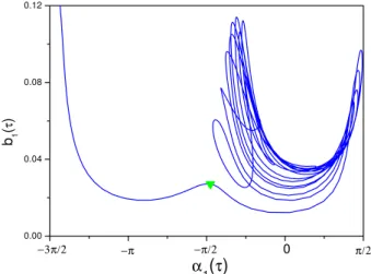
To understand what happens at the turning point we in-voke Eqs. (5) again, but now we need the knowledge on the modes ofδφ (ξ, τ ). Our investigation shows that the master oscillator, i.e. ofk=1, plays a critical role in this respect. For the same case of Fig. 5, we plotb1(τ ) vs.α1(τ )in Fig. 6,
in which the triangle corresponds exactly to the same criti-cal moment at the turning point in Fig. 5. One can see that corresponding to the cyclic motion in Fig. 5, in Fig. 6b1(τ )
vs.α1(τ )makes vibrations like a nonlinear pendulum with
α1(τ )confined in a range much less than 2π. Right at the
critical moment of the turning point in Fig. 5, the orbitb1(τ )
vs.α1(τ )moves to the top of a hump in Fig. 6, after which
α1(τ ) no longer simply vibrates, instead it may cross over
0.00 0.04 0.08 0.12
π/2 0
−π/2 −π
−3π/2
b1
(
τ
)
α1
(
τ)
Fig. 6. Motion of the master modeb1(τ )vs.α1(τ ), the same
tran-sient period as in Fig. 5. The triangles in Figs. 5 and 6 correspond to the same moment.
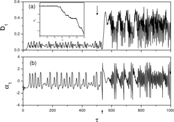
2π as well. The latter fact can be seen more clearly in Fig. 7 for temporal evolutions of Fig. 7ab1(τ )and Fig. 7bα1(τ ).
The arrows in Figs. 7a and b correspond to the critical times for the two dynamic events, i.e. the collision and the turn-ing point, respectively. One can see in Fig. 7b that after the second eventα1(τ ) can make vibrating as well as whirling
motion (here mod(2π )has been taken), in contrast, before the second eventα1(τ )vibrates within a small range. In the
inset we plotα1(τ )without taking mod(2π ), one can see that
after the second eventα1(τ )steps down continuously.
The above results convince us that there are two critical dynamic events involved in the crisis-induced transition to the spatiotemporal chaos: the first one is a collision with the saddle point which triggers the crisis, the subsequent one is a state transition ofk=1 mode phase, that is, its motion changes from a purely nonlinear vibration to a combined motion of whirling and vibrating, it is the latter event that directly spoils the spatial coherence and leads to the spa-tiotemporal chaos. In the calculations with different initial conditions we always observed the similar turning point and hump as the ones in Figs. 5 and 6, respectively, in particular the tops of the humps correspond to the same value ofα1, i.e.
α1∗≈−1.54 (with 3.9% relative error in 20 test runs), suggest-ing that at this place there might be a saddle with a separatrix dividing the vibration and vibration-whirling regimes ofα1,
probably the second event is caused by a collision with this saddle.
3 Functional relations between the modes in spatially regular wave before transition
In the last section we transformed nonlinear wave Eq. (1) into a set of coupled oscillators{bk(τ ), αk(τ )}moving in a potentialφ0(ξ ), this transformation has greatly simplified the
0 200 400 600 800 1000 -4
-2 0 2 4 0.0 0.2 0.4
(b)
b 1
α 1
τ
(a)
0 200 400 600 800 1000 1200 -150
-100 -50 α1
τ
Fig. 7. Temporal evolution of (a) b1(τ ) and (b) α1(τ ) for
=0.65, ε=0.22, the two arrows indicate the critical times for the collision with the saddle point (the first critical event) and for the orbit ejected to the spatiotemporally chaotic attractor (the second critical event), respectively. The inset showsα1(τ )without taking
mod(2π ).
therefore be considered as the results of self-organization of the oscillators.
As is well known coupled nonlinear oscillators may adjust themselves to a PS under certain conditions, i.e. their phase difference|△βmn(τ )|≡|βm(τ )−βn(τ )|is constrained in a fi-nite range (Fujisaka and Yamada, 1983; Pecora and Carroll, 1990; Rosenblum et al., 1996, 1997; Boccaletti et al., 2002). If asymptotically△βmnis zero, the oscillators reach a com-plete PS; more generallyβm(t )may show a functional PS withβn(t ), i.e. while△βmn(τ )is small, a functional relation βm(t )=F[βn(t )]is hold. In addition, a PS can be perfect or imperfect, for example, it is found that in coupled Lorenz os-cillators, although the phase difference looks very erratic it can be confined in a finite range less than 2πfor a long time, and occasionally a phase slip may occur (Zaks et al., 1999).
Now let us compare the behaviors before and after the tran-sition in our system in terms of PS. In the present section the spatially regular states forε<εc will be discussed. In our case the simplest spatial regular wave is a stable steady wave. From Eq. (5) with a saddle steady waveφ0∗(ξ )as the potential, in certain parameter regimes we can find nontrivial constant solutions of{bk(τ→∞), αk(τ→∞)} correspond-ing to a stable steady waveφ0(ξ ), in which asymptotic phase
difference△αkk′(τ→∞)≡αk(τ )−α
k′(τ )|τ→∞between any two oscillators is constant.
With variation of parameters △αkk′(τ ) can no longer
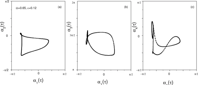
hold as constants, however, the oscillators are still able to adjust themselves to perfect functional PS. For =0.65, ε=0.12 Fig. 8 depicts Fig. 8a energy of the os-cillators, δE(τ )=Pk(1−ak2)[Akbkcos(θk−αk)/2+bk2/4], Figs. 8b–d phase difference△α1k(τ )fork=2,3,4, respec-tively. One can see that all the△α1k(τ )are confined within a finite range less than 2π. For the same parameters in Fig. 9 we plotαk(τ )vs.α1(τ )with Figs. 9a–c fork=2,3,4,
respec-3000 3200 3400 3600 3800 4000 -0.10
-0.05
−π 0 π 0 π 2π −π
0 π
∆α
14
τ
∆α
13
∆α
12
(d) (c) (b) (a)
Ω=0.65, ε=0.12
δ
E
Fig. 8. Temporal evolution of(a) δE(τ ), (b)–(d) △α1k(τ ) for
k=2,3,4, respectively,=0.65, ε=0.12<εc.
tively, they all show smooth curves, indicating that the oscil-lators have established a perfect functional PS collectively. As a result of the functional PS, δE varies periodically as can be seen in Fig. 8a.
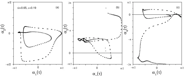
With increasing ε the functional PS curves in the phase plot αk(τ ) vs. α1(τ ) become more and more
compli-cated, and phase slips may occur in some oscillators. For =0.65, ε=0.19. Figure 10 showsαk(τ )with Fig. 10ak=1 (black), 2 (red), 4 (green) and Fig. 10bk=1 (black), 3 (pink). In the calculation mod(2π ) is taken only when τ <3000. One can see that in Fig. 10a, roughly speaking, bothk=2,4 modes are synchronized withk=1 mode, occasionallyk=4 mode experiences a phase slip but it is soon locked back to the domain of α1(τ )again; on the other hand, in Fig. 10b
α3(τ )is no longer locked to the domain ofα1(τ ), which
in-creases with time, in contrast to constant average ofα1(τ ).
However, if taking mod(2π )forα3(τ )orα4(τ ), respectively,
one would find that functional relations of their motion with that of the other modes still remain. Figure 11 shows the phase plotαk(τ )vs.α1(τ )(k=2,3,4 in Figs. 11a–c,
respec-tively) for the same case as in Fig. 10 but with the mod(2π ) taken, in all the plots we obtain smooth curves, that is, they have perfect functional relations. In the inset of Fig. 10b we show △ α13(τ )≡α1(τ )−α3(τ ), one can see that the phase
slip ofα3(τ ) relative toα1(τ ) occurs nearly in every
char-acteristic period, nevertheless the staircase-like behavior of
△ α13(τ ) suggests thatα3(τ ) also reaches a kind of
func-tional PS withα1(τ ).
(a)
Ω=0.65, ε=0.12
−π/2 0 π/2
−π/2
π/2
0
α 2
(
τ)
α
1
(
τ)
(b)
2π
3π/2
π
−π/2 0 π/2
α 3
(
τ
)
α1
(
τ)
(c)
−π/2 0 π/2
−π/2 π/2
0
α 4
(
τ
)
α
1
(
τ)
Fig. 9.αk(τ )vs.α1(τ )for the same case as in Fig. 8,(a)–(c)are fork=2,3,4, respectively.
3000 3200 3400 3600 3800 4000 0
100 200 -10 -5 0 5
3000 3020 3040 3060 3080 3100 -40
-30 -20 -10 0
(b)
α 1
,
α 3
τ
(a) Ω=0.65, ε=0.19
α 1
,
α 2
,
α 4
∆α13(τ)
Fig. 10. Temporal evolution ofαk(τ ) for(a)k = 1 (black), 2
(red), 4 (green),(b) k=1 (black), 3 (pink),=0.65, ε=0.19<εc.
The inset shows△α13(τ ).
φ0∗(ξ )can still adjust their relative relations in a perfect func-tional way, producing a wave that is erratic in time while maintaining the spatial coherence.
4 On-off imperfect phase synchronization in spatiotem-poral chaos
The wave state after the transition is extremely irregular both in time and in space. It is remarkable that even in such turbu-lent waves one can observe PS. However, now the synchro-nization is characterized by its imperfection (He and Chian, 2003). Just like in coupled Lorenz oscillators (Zaks et al., 1999), a turbulent wave in our system has an embedded sad-dle point, which has a characteristic time scale unbounded from above, the oscillators are not easy to adjust to a perfect PS.
Figure 12 is an example with=0.65, ε=0.22>εc, where Fig. 12a is the temporal evolution of δE(τ ), Figs. 12b–d are phase differences △α1k(τ ) for k=2,3,4, respectively. One can see that in δE(τ ) there are many sharp spikes, corresponding to each sharp spike in Fig.12a, all the phase differences △α1k in Figs. 12b–d are varying erratically in a very small range; in contrast, between two sharp spikes δE(τ )oscillates in a lower level and△α1k can become very large, even surpassing 2π, (in Figs. 12b–d mod(2π )has been taken). That is, in this turbulent wave the phasesαk(τ )can adjust to imperfect PS intermittently. We name this behavior as an on-off collective imperfect PS (He and Chian, 2003).
The correspondence between the spikes inδE(τ )and im-perfect PS inαk(τ )is significant, which suggests that bursts in the wave energy are induced by the imperfect PS “on”. To further confirm this point, let us observe the motion of the mode amplitudes {bk(τ )}. An individual bk(τ ) looks very chaotic, however, if putting different mode amplitudes to-gether one would find that synchronization may also exist among them. Figure 13 is for the same parameters as in Fig. 12, with Fig. 13aδE(τ ), Fig. 13bαk(τ )fork=1,2 and Fig. 13cbk(τ )fork=1,2,3, respectively. In the plot one can see that, while the phases{αk}adjust to a synchronization the amplitudes {bk}reach maximum about simultaneously, due to effective building up of the mode energies, a burst ap-pears inδE(τ ), respectively in “on” stages of imperfect PS. This phenomenon is very different from that of spatially reg-ular state before the transition. For a spatially regreg-ular wave, a PS among the oscillators is perfect (see Figs. 9 and 11); besides, due to the functional relation between them, nor-mally the peaks of δE(τ ) do not show correspondence to small△αkk′(τ ), and{bk(τ )}do not reach maximum
(a)
Ω=0.65, ε=0.19
−π/2 0 π/2
−π/2 0
α 2
(
τ
)
α1(τ)
0
(b)
π
−π/2
−π/2 0 π/2
α3
(τ
)
α1(τ)
0
(c)
−π/2 0 π/2
−2π −π
α 4
(
τ
)
α1(τ)
Fig. 11.αk(τ )vs.α1(τ )for the same case as in Fig. 10,(a)–(c)are fork=2,3,4, respectively, mod(2π )has been taken.
up by its mode energies of different scales, although only in short periods of time. In the “on” stages a best cooperation is realized between the oscillators.
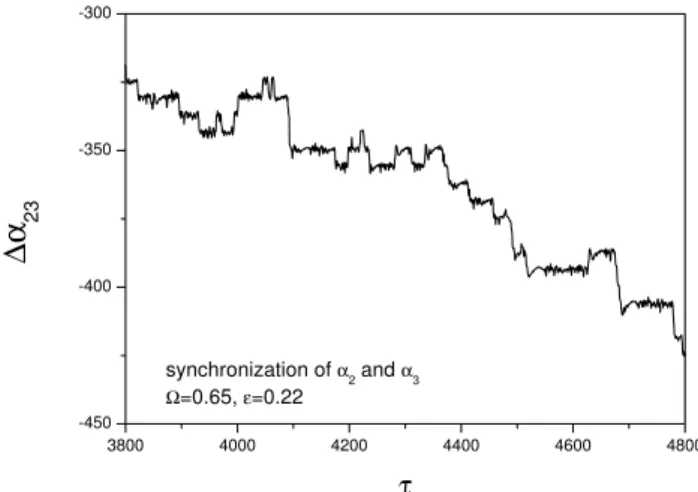
In Fig. 14 we plot temporal variation of △α23(τ )
with-out taking mod(2π ), some plateaus can be seen in the curve, which correspond to the “on” stages of collective imper-fect PS; between two plateaus|△α23|increases very quickly,
which are the “off” stages of the PS. Because of the multi-dimensions of our system, the plateaus are not as flat as in the coupled Lorenz oscillators (Zaks et al., 1999), and usually in our case the oscillators take a longer time to adjust to a new plateau again.
As we have seen in Sect. 2, both before and after the crisis the system has a saddle point, so the different PS behaviors in the spatially regular wave and spatiotemporal chaos can not be explained only by the existence of saddle point. Notice that owing to the second dynamic event thek=1 oscillator experiences a trapped-free transition, delocalization of this master mode is also crucial for these different behaviors. Be-fore the transition the motion of{bk, αk}is strongly governed by the potentialφ0∗(ξ ), a functional relation is then formed between the modes; after the transition, the k=1 mode – which slaves the other modes – can be free from the poten-tial, in the meantime the amplitudes{bk}grow greatly, in this case the potential has less influence and so the oscillators have a stronger tendency to adjust by themselves, as a result an on-off collective imperfect PS is established.
In the “on” stages of collective imperfect PS△αkk′ is near
0 orπ, this fact allows us to define a correlation function between the phases ofNoscillators
CαN(τ )= N Y
k=1
|cosαk(τ )|.
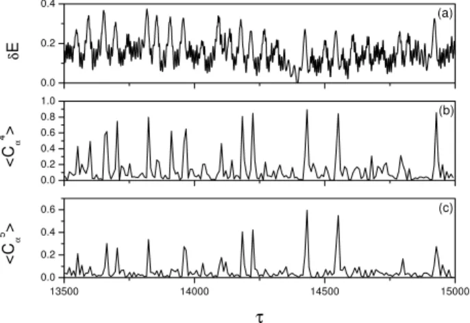
Figure 15 shows (a) the wave energyδE(τ ), (b)hC4α(τ )i, (c) hC5α(τ )i, herehidenotes time-average in a characteristic pe-riod. In the plot correspondence between the sharp spikes ofδE(τ )and that ofhCαN(τ )iis obvious, in particular in (b) hC4α(τ )ishows strong spikes whenever there appears a burst
2750 3000 3250 3500 3750 -4
-2 0 2 4 0 2 4 6 -4 -2 0 2 4 0.0 0.1 0.2 0.3 0.4
∆α
14
τ
∆α
13
∆α
12
off on
(d) (c) (b) (a)
δ
E
Fig. 12. Temporal evolution of(a)δE(τ ),(b)–(d)△α1k(τ )for
k=2,3,4, respectively, =0.65, ε=0.22>εc. One can see that
whenever imperfect PS occurs a strong burst appears inδE(τ ).
inδE(τ ). In (c) the spikes ofhCα5(τ )iare still apparent, but is not as prominent as inhCα4(τ )i. If more and more modes are included the spikes inhCαN(τ )iis gradually smeared out. It is likely that the best synchronization occurs among a few long wavelength modes. Apart from those strong spikes there are also smaller peaks inhCαN(τ )i, the correspondence be-tween the peaks ofhCαN(τ )iand that ofδE(τ )is also clear. These results indicate that in the turbulent state after the cri-sis, an instant wave energy significantly depends on the rela-tive phase status of the oscillators, in particular when the os-cillators adjust to a collective imperfect PS the total energy displays a strong burst.
13800 13850 13900 13950 14000 0.0
0.4 0.8 -4 -2 0 2 4 0.0 0.2 0.4
(c)
bk=
1
-3
τ
(b)
α1
,
α2
+
π
(a)
δ
E
Fig. 13. Temporal evolutions of(a)δE(τ ),(b)αk(τ )(k = 1,2)
and(c)bk(τ )(k=1−3), for=0.65, ε=0.22, black/green/red line
is fork=1,2,3, respectively.
5 Conclusion and discussion
To investigate nonlinear dynamics of the drift-wave system, we transform the nonlinear wave into a set of coupled lators in the potential of a steady wave solution. These oscil-lators contribute the active part of the wave. In particular the motion of oscillators in the potential of a saddle steady wave is studied, the latter is a saddle point in its moving frame. It is shown that a collision with the saddle point (or equivalently a “pattern resonance” with the embedded saddle steady wave) triggers a crisis, which then induces a subsequent event that destroys the spatial regularity of the wave.
The phase dynamics is investigated for the states before and after the crisis-induced transition. We find that in the very turbulent state after the transition the oscillators have a strong tendency of adjusting to PS, as a result an on-off imperfect PS can be established. As a comparison in the spa-tially regular states before the transition, perfect functional PS among the oscillators are observed with or without phase slips. The different behaviors of mode phases can be under-stood if taking into account the effect of the saddle steady wave potentialφ0∗(ξ ), which strongly governs the motion of the oscillators before the transition but has less influence af-ter it. In the lataf-ter case the masaf-ter mode can be free of the potential, the orbits of oscillators are no longer restricted by a simple functional relation, instead they have more opportu-nities to adjust their amplitudes and phases, consequently a special on-off collective imperfect PS is formed.
The transformation of nonlinear wave Eq. (1) into Eq. (4) is mathematically strict, besides, when obtaining the coupled oscillators Eqs. (5) we did not make further assumption for the wave solutions except for the periodicity. The dynamic phenomena observed in Eq. (5) with appropriate truncation are in agreement with that of Eq. (1). One can therefore be-lieve that the phase dynamics obtained in Eq. (5) reveals the physical process in nonlinear wave Eq. (1).
When dealing with turbulence, usually a random-phase
as-3800 4000 4200 4400 4600 4800 -450
-400 -350 -300
synchronization of α2 and α3 Ω=0.65, ε=0.22
∆α
23
τ
Fig. 14. Temporal evolution of△α23(τ )for=0.65, ε=0.22 without taking mod(2π ).
sumption is adopted in statistical investigations. However, our results indicate that the mode phases are not really ran-dom even in a very turbulent state. In our case phases{αk} are of the oscillators, which are obtained after transforming to the moving frame and subtracting the saddle steady wave. Nevertheless, it is evident now that different spatial scales in a turbulence are not statistically uncorrelated, on the con-trary, they may intermittently show very strong correlations both in their amplitudes and phases, the instant correlations can be even stronger than in spatially regular waves. That is why energy bursts show up in the turbulent waves rather than in spatially regular ones. In the real world similar energy bursts can be seen in many turbulent systems, e.g. swells in ocean, flares in the sun, sharp spikes in brain electric signals ..., can these bursts also be attributed to mode energy build-ing up in “on” stages of the PS? If this is proved to be true, on-off collective imperfect PS may provide a potential ap-plication in predicting occurrence of energy bursts in these systems. For instance, solar flares are considered as a re-sult of nonlinear solar turbulent plasmas, furthermore, they display the same statistics as that ofCαN, e.g. probability dis-tribution of interspikes of the flares also follows a power law (Boffetta et al., 1999). If on-off collective imperfect PS is shown to be the mechanism of solar turbulence, in principle solar flares should be predictable. However, to this end we may need the knowledge of, e.g. the embedded saddle steady wave, with which one is able to transform the system to the moving frame and work out the motion of oscillators that constitute the active part of the turbulent wave. Obviously for practical application we still face many difficulties.
13500 14000 14500 15000 0.0
0.2 0.4 0.6 0.0 0.2 0.4 0.6 0.8 1.0 0.0 0.2
(c)
<C
α
5 >
τ
(b)
<C
α
4 >
δ
E
Fig. 15.Temporal evolution of(a)δE(τ )and(b),(c)hCαN(τ )ifor
N=4,5, respectively,=0.65, ε=0.22. The correspondence of the bursts inδE(τ )with spikes ofhCα4(τ )iis very clear.
of magnetohydrodynamic turbulence in the earth´s foreshock region, and showed that the correlation of wave phases exists which provides an evidence of nonlinear wave interactions (Hada et al., 2003). Koga and Hada applied the wavelet anal-ysis to show that although the magnetohydrodynamic turbu-lence in the Earth´s foreshock region is consisted of waves of a wide frequency range, only frequencies lower than the ion gyrofrequency are responsible for generating the phase coherence (Koga and Hada, 2003). Schulz et al. suggest that phase synchronization of different climate cycles can ex-plain glacial-interglacial contrast in ocean climate variability (Schulz et al., 2004). The space observation of Hada et al. (2003) and Koga and Hada (2003) and the ocean model of Schulz et al. (2004) are in agreement with our theoretical re-sults that in general PS plays an important role in nonlinear wave systems. In particular, our result on the on-off collec-tive imperfect PS may help for further investigation on syn-chronization of different spatial scales in very turbulent sys-tems.
Acknowledgements. This work is supported by the Special Funds
for Major State Basic Research Projects of China and by the NSFC No. 10475009 and No. 10335010, by RFDP No. 20010027005 in China, and by CNPq in Brazil.
Edited by: P. Chu Reviewed by: one referee
References
Benjamin, T. B., Bona, J. L., and Mahony, J. J.: Model equations for long waves in nonlinear dissipative systems, Philos. Trans. Roy. Soc. London Ser. A, 272, 47–78, 1972.
Bishop, A. R., Fesser, K., Lomdahl, P. S., Kerr, W. C., Williams, M. B., and Trullinger, S. E.: Coherent spatial structure versus time chaos in a perturbed Sine-Gordon system, Phys. Rev. Lett., 50, 1095–1098, 1983.
0.1 1
1E-3 0.01 0.1
P
τL
Fig. 16. Distribution function,P (τL), of interspikeτLofhCα4(τ )i
for=0.65, ε=0.22, which shows a power law behavior as fitted by the solid line.
Biskamp, D. and He, K.: Three-drift-wave interaction at finite par-allel wavelength: bifurcation and transition to chaos, Phys. Flu-ids, 28, 2172–2180, 1985.
Boccaletti, S., Kurths, J., Osipov, G., Valladares, D. L., and Zhou, C. S.: The synchronization of chaotic systems, Phys. Rep., 366, 1–101, 2002.
Boffetta, G., Carbone, V., Giuliani, P., Veltri, P., and Vulpiani, A.: Power laws in solar flares: Self-organized criticality or turbu-lence?, Phys. Rev. Lett., 83, 4662–4665, 1999.
Chat´e, H. and Manneville, P.: Transition to turbulence via spatio-temporal intermittency, Phys. Rev. Lett., 58, 112–115, 1987. Chern, C. and I, L.: Multiplicity of bifurcation in weakly ionized
magnetoplasmas, Phys. Rev. A, 43, 1994–1997, 1991.
Chian, A. C.-L., Rempel, E. L., Macau, E. E., Rosa, R. R., and Cris-tiansen, F.: High-dimensional interior crisis in the Kuramoto-Sivashinsky equation, Phys. Rev. E, 65, 035203(R)-1-4, 2002. Chian, A. C.-L. and the WISER team: Foreword: advances in space
environment research, Space Science Rev., 107, 1–3, 2003. Chian, A. C.-L., Borotto, F. A., Rempel, E. L., Macau, E. E. N.,
Rosa, R. R., and Christiansen, F.: Dynamical systems approach to space environment turbulence, Space Science Rev., 107, 447– 461, 2003.
Cross, M. C. and Hohenberg, P. C.: Pattern formation outside of equilibrium, Rev. Mod. Phys., 65, 851–1112, 1993.
Dodd, R. K., Eilbeck, J. C., Gobbon, J. D., and Morris, H. C.: Soli-tons and nonlinear wave equations, Academic Press, London, 596, 1982.
Eckmann, J. -P.: Roads to turbulence in dissipative dynamical sys-tems, Rev. of Mod. Phys., 53, 643–654, 1981.
Foss, J., Longtin, A., Mensour, B., and Milton, J. : Multistability and delayed recurrent loops, Phys. Rev. Lett., 76, 708–711, 1996. Frisch, U.: Turbulence, Cambridge University Press, Cambridge,
1995.
Fujisaka, H. and Yamada, T.: Stability theory of synchronized mo-tion in coupled-oscillator systems, Prog. Theor. Phys., 69, 32–47, 1983.
Hada, T., Koga, D., and Yamanoto, E.: Phase coherence of MHD waves in the solar wind, Space Science Rev., 107, 463–466, 2003.
Korteweg-de Vries equation, Phys. Lett. A, 132, 175–178, 1988. He, K. and Salat, A.: Hysteresis and onset of chaos in periodically driven nonlinear drift waves, Plasma Phys. Contr. Fusion, 31, 123–141, 1989.
He, K.: Crisis-induced transition to spatiotemporally chaotic mo-tions. Phys. Rev. Lett. 80, 696–699, 1998.
He, K.: Saddle pattern resonance and onset of crisis to spatiotem-poral chaos, Phys. Rev. Lett., 84, 3290–3293, 2000.
He, K. and Chian, A. C. -L.: On-off collective imperfect phase syn-chronization and bursts in wave energy in a turbulent state, Phys. Rev. Lett., 91, 034102-1-4, 2003.
He, K.: Hopf bifurcation in a nonlinear wave system, Chin. Phys. Lett., 21, 439–442, 2004.
He, K. and Chian, A. C. -L.: Critical dynamic events at the crisis of transition to spatiotemporal chaos, Phys. Rev. E, 69, 026207-1-12, 2004.
Horton, W.: Nonlinear drift waves and transport in magnetized plas-mas, Phys. Rep., 192, 1–177, 1990.
Infeld, E. and Rowlands, G.: Nonlinear waves, solitons and chaos, Cambridge University Press, Cambridge, 1990.
see, for example, Principles of Neural Science, edited by Kandel, E. R., Schwartz, J. H. and Jessell, T. M., The Mc Graw-Hill Com-panies, Inc., 938, 2000.
Kim, S., Park, S. H., and Ryu, C. S.: Multistability in coupled oscil-lator systems with time delay, Phys. Rev. Lett., 79, 2911–2914, 1997.
Klinger, T., Latten, A., Piel, A., Bonhomme, G., Pierre, T., and Dudok de Wit, T.: Route to drift wave chaos and turbulence in a bounded low-βplasma experiment, Phys. Rev. Lett., 79, 3913– 3916, 1997.
Koga, D. and Hada, T.: Phase coherence of foreshock MHD waves: wavelet analysis, Space Science Rev., 107, 495–498, 2003.
Lichtenberg, A. J. and Lieberman, M. A.: Regular and Chaotic dy-namics, Springer, Berlin), 1983.
Nakatsuka, H., Asaka, S., Itoh, H., Ikeda, K., and Matsuoka, M.: Observation of bifurcation to chaos in an all-optical bistable sys-tem, Phys. Rev. Lett., 50, 109–112, 1983.
Ott, E.: Chaos in dynamical systems, Cambridge University Press, New York, 277, 1993.
Park, E.-H., Zaks, M. A., and Kurths, J.: Phase synchronization in the forced Lorenz system, Phys. Rev. E, 60, 6627–6638, 1999. Pecora, L. M. and Carroll, T. L.: Synchronization in chaotic
sys-tems, Phys. Rev. Lett., 64, 821–824, 1990.
Rosenblum, M. G., Pikovsky, A. S., and Kurths, J.: Phase synchro-nization of chaotic oscillators, Phys. Rev. Lett., 76, 1804–1807, 1996.
Rosenblum, M. G., Pikovsky, A. S., and Kurths, J.: From phase to lag synchronization in coupled chaotic oscillators, Phys. Rev. Lett., 78, 4193–4196, 1997.
Schulz, M., Paul, A., and Timmermann, A.: Galcial-interglacial contrast in climate variability at centennial-to-milennial timescales: observations and conceptual model, Qua-ternary Science Rev., 23, 2219–2230, 2004.
Sun, H., Ma, L., and Wang, L. : Multistability as an indication of chaos in a discharge plasma, Phys. Rev. E, 51, 3475–3479, 1995. Swinney, H. L.: Observation of order and chaos in nonlinear
sys-tems, Physica D, 7, 3–15, 1983.
Zaks, M. A., Park, E. -H., Rosenblum, M. G., and Kurths, J.: Alter-nating locking ratios in imperfect phase synchronization, Phys. Rev. Lett., 82, 4228–4231, 1999.