SRef-ID: 1432-0576/ag/2004-22-2283 © European Geosciences Union 2004
Annales
Geophysicae
Magnetic turbulent spectra in the magnetosheath: new insights
F. Sahraoui1, G. Belmont1, J. L. Pinc¸on2, L. Rezeau1,3, A. Balogh4, P. Robert1, and N. Cornilleau-Wehrlin1
1Centre d’Etude des Environnements Terrestre et Plan´etaires, 10/12 avenue de l’Europe, 78140, V´elizy, France 2Laboratoire de Physique et de Chimie de l’Environnement, 3A avenue de la Recherche Scientifique, Orl´eans, France 3Also at Universit´e Pierre et Marie Curie, Paris, France
4Space and Atmospheric Group, The Blackett laboratory, Imperial College, Prince Consort road, London, UK
Received: 24 February 2004 – Revised: 6 April 2004 – Accepted: 20 April 2004 – Published: 14 June 2004
Abstract. The spectrum of the magnetic fluctuations mea-sured by the Cluster satellites in the inner magnetosheath is investigated using the k-filtering technique. On a case study, it is shown first that the wave vectors calculated from the Flux Gate Magnetometer (FGM) data fit well with those de-termined from the Spatio-Temporal Analysis of Field Fluc-tuations (STAFF) data for their common range of frequency, which allows one to confirm that the high pass filter applied to STAFF data does not alter the spatial characteristics of its spectra. Both analyses confirm the dominance of the mirror mode for frequencies up to 1.4 Hz. Furthermore, by com-paring the experimental charateristics of the identified mir-ror mode to the prediction of the linear theory, it is shown that the predicted maximum growth rate is observed in the frequency range 0–0.15 Hz, i.e. the FGM range. All the rest of the mirror mode, identified for higher frequencies is more likely to be a non linear extension of the most instable one. This cascade on the spatial scales is, in turn, observed in the satellite frame as a temporal spread due to Doppler shift. Fur-ther implications on the real nature of the observed spectrum are discussed.
Key words. Magnetospheric physics (magnetosheath, plasma waves and enstabilities). Space plasma phusics (turbulence)
1 Introduction
The magnetic turbulence in the terrestrial magnetosheath plays a key role in the dynamical coupling between the so-lar wind and the magnetosphere. It has been investigated for many years both experimentally (Hubert et al., 1989; Gleaves and Southwood , 1991; Song et al., 1994; Denton et al., 1995; Constantinescu et al., 2003) and theoretically (Omidi and Winske, 1995; G´enot et al., 2001; Hellinger et al., 2003). Now, thanks to the availability of the multipoint measure-Correspondence to:F. Sahraoui
(fouad.sahraoui@cetp.ipsl.fr)
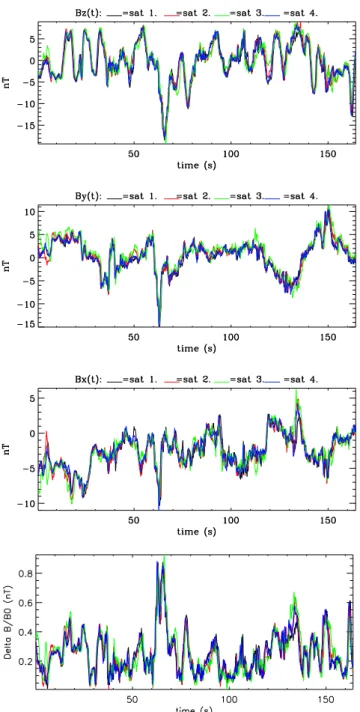
Fig. 1. The magnetic field components measured by the FGM ex-periment in the MFA frame. The continuous components are re-moved from the data and used to define the MFA frame. The three first panels (from top to bottom) represent respectively the parallel and the perpendicular components of the magnetic fluctuations. The last one shows the modulus of the magnetic fluctuations normalized to the background magnetic field. The color code is relative to the four satellites.
2 Observations
The data used in the present study have been gathered by the Cluster spacecraft on 18 February 2002 in the inner mag-netosheath around 05:34 (LT). The crossing of the magne-topause by the spacecraft was about 35 min before. The
lite spin at 0.25 Hz. Therefore, to avoid any problems relative to this last point, we use the FGM data to prolong the study to frequencies below 0.35 Hz. In the present work, we inves-tigate the magnetic turbulence in the frequency range 0.2 Hz: FGM data are used from 0 to 0.35 Hz, whereas STAFF data are used from 0.35−2 Hz. This will allow one to com-plete the first study done by Sahraoui et al. (2003), which used STAFF data only and analysed the frequency range 0.35−1.2 Hz. Now, we will particularly focus on the fre-quency range 0,0.5 Hz, and two main goals are checked: first we check whether the high pass filter (withfcut−off=0.35 Hz)
that had been applied to STAFF data did not alter the physi-cal results provided by the k-filtering method. This is done by comparing the nature of the identified waves in the frequency range 0.35−0.5 Hz covered by both experiments. Then, we will study from FGM data the nature of the new waves that could appear for frequencies lower than 0.35 Hz. This last purpose will allow, as we can see below, one to answer some questions that have been raised in the first work of Sahraoui et al. (2003).
In Fig. 1 the X, Y, and Z magnetic waveforms from FGM experiment in the MFA frame over about 164 s are shown. As one can see, the parallel componentBzshows low amplitude oscillations of about a 10-s period, more clearly observable during the first 60 s and between 90 to 150 s.
These dominant oscillations can also be seen on the FFT spectrum of the parallel component shown in Fig. 2. In fact, up to 0.2 Hz, the parallel component dominates the perpen-dicular one with a significant enhancement around the fre-quency 0.1 Hz. Between 0.2 to 0.6 Hz, the parallel compo-nent is slightly larger than the perpendicular one and exibits more oscillations. From 0.6 up to 2 Hz the two components have comparable levels and both exhibit small peaks. The dominance of the parallel component in the LF part of the spectrum can be taken as a signature of compressible waves. These issues will be clarified in the next section.
3 Wave identification using the k-filtering technique
Fig. 2. The FFT spectra calculated from FGM data for the fre-quency range [0.07, 2] Hz. The parallel component (red line) is compared to the perpendicular one (blue line), and to the whole spectrum (black line).
time series. In real data, these two hypotheses are never strictly fulfilled. However, in practice, we are content with the concept of weak space (time) homogeneity (stationarity): the signal should be homogeneous (stationary) on scales that are larger than the largest spatial (temporal) scale determined by the k-filtering method. Obviously, the determination of the wave vectorskfrom spatially undersampled data (even the Cluster ones) is not trivial. The k-filtering technique uses a sophisticated method to overcome this difficulty: it intro-duces nonlinear filters for each couple(ω,k), requiring that all the energy contained in the signal is absorbed except that related to(ω,k)(Pinc¸on and Motschmann, 1998). The va-lidity domain of the technique in the wave vector space is de-termined from the separations between the Cluster satellites: all the existing wavelengths have to be larger than the space-craft separations, which are of the order of 100 km in the present case. Once the magnetic energy distributionP (ω,k) is calculated, it can be used to identify the existing propagat-ing modes (Sahraoui et al., 2003): for each given frequency ω0, and using an isocontour representation, the distribution
of energy ink-space is displayed as cuts in the(kx, ky)plane along thekzaxis. For eachkzcorresponding to an identified peak, the theoretical dispersion relations of the plasma LF linear modes (MHD and mirror modes) are then superposed after being Doppler shifted using the flow velocities from the CIS experiment (R`eme et al., 1997). The mirror mode is as-sumed to have approximately a zero frequency in the plasma frame, which means that it is observed in the satellite frame with the dispersion ω=k.v. The dispersion relations are computed using the WHAMP program (R¨onnmark, 1982), where the control parameters are those measured by the dif-ferent Cluster experiments:B0from FGM, ion temperatures
from CIS, and plasma density from WHISPER (D´ecreau et al, 1997). For more details on the previous results, the reader is referred to Sahraoui et al. (2003). Application of the k-filtering technique to the frequency f=0.44 Hz, ac-cessible on FGM and STAFF data, allows for the identi-fication of an isolated peak shown in Fig. 3. The energy distributions determined from the two experiments look
al-Fig. 3. Comparison of the energy distribution in kspace of the most intense identified peak for the frequency f=0.44 Hz from FGM (top panel) and STAFF (bottom one). The black thin lines are the isocontours of energy in the(kx, ky) plane, whereas the colored lines are the theoretical dispersion relations of the LF modes. The blue line is the Doppler shiftω=k.vand corresponds to the mirror dispersion relation in the satellite frame. Alfv´en and slow modes (red lines) are very close to the mirror dispersion curve in this case of a quasi-perpendicular direction of propagation.
most identical: the two peaks are, respectively, centred on the wave vectorskF GM=(−142.5,51.7,−7.1)×10−4rd/km and kSTAFF=(−127.5,51.7,−7.1)×10−4rd/km. The two
wave vectors are separated by an angle less than 3◦. This
kvth///wcp
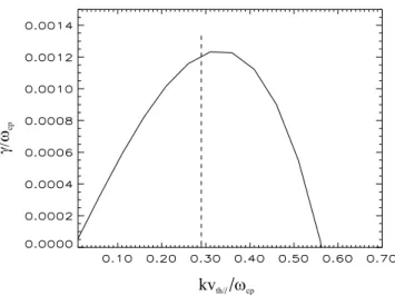
Fig. 4. The linear growth rate calculated from WHAMP using the measured parameters for the angle(k,B0)=80◦. vth//=154 km/s is the parallel thermal velocity of the protons,ωcp=2.07 rd/s is their
cyclotron pulsation. The vertical dashed line shows the location of the experimental wave vector of the most intense identified mirror mode.
Fig. 5. The most intense peak identifiable on the whole spectrum 0–10 Hz. It is observed at f=0.11 Hz centred on the mirror mode dispersion curveω=k.v(blue curve). Its wave vectorkhas an angle −80◦withB0and a modulus k=0.00389 rd/km. Alfv´en and slow modes (straight red curve) are degenerated and very close toω=k.v.
4 Discussion
Now let us look at the physical properties of the whole spec-trum: 0−0.35 Hz from FGM and 0.35−2 Hz from STAFF. As we can see in Fig. 3, which shows thek-energy distri-bution for the observed frequency f=0.44 Hz, the identified peak is localized on the lineω=k.vwhich corresponds to the dispersion relation of the mirror mode in the satellite frame (ω∼0 in the plasma frame). Its wave vector makes a−80◦ angle with respect to the local magnetic field.
Ap∼1.28.
In Fig. 4 the linear growth rate of the mirror instabil-ity is shown as a function of the wave vector for the angle θ=(k,B0)=80◦.
The theoretical maximum growth rate is obtained for the value kγmax=0.004 rd/km. Although the measured param-eters are very close to the marginal instability threshold (Ap∼1.28, β⊥∼4), the theoretical value is three times less
than the observed modulus of the mirror mode wave vector k=0.0124 rd/km associated with the satellite frame frequency (f=0.37 Hz) studied by Sahraoui et al. (2003). This discrep-ancy between the observations and the basic linear theory of the mirror mode was pointed out in that work, and has re-mained unanswered since then.
Now, to solve this problem, we notice first that the mir-ror mode is observed in the quasi-perpendicular direction, its dispersion relation can be written asωobs=k.v∼k⊥v⊥.
Ac-cordingly, one may expect to observe increasingk⊥with
in-creasing frequencies in the satellite reference frame. This point was indeed verified in Sahraoui et al. (2003), since the identified peaks have largerk for higher frequencies in the frequency range 0.35−1.2 Hz. These observations, therefore, support that the mirror instability would actually develop for frequencies lower than 0.35 Hz, and would be observable for higher frequencies only by Doppler shift.
To check the validity of this interpretation, we look at the results of the k-filtering technique obtained in the frequency range 0,0.35 Hz from FGM data. The most intense peak is identified at the frequency f=0.11 Hz in the satellite refer-ence frame, which corresponds to the 10-s period oscillating waves previously seen on the parallel component of the fluc-tuations (Fig. 1) and explains the energy enhancement on the parallel spectrum atf∼0.1 Hz (Fig. 2). This most intense peak, shown in Fig. 5, lies on the dispersion curve of the mir-ror modeω=k.v. The corresponding wave vectorkmakes a−80◦angle withB
0and its modulus is k=0.00389 rd/km.
out to be observed in the satellite frame as a temporal effect by Doppler shift. The mirror mode spectrum could also ex-tend to frequencies higher than 1.4 Hz, but the corresponding wave vectors are not accessible to measurement because of the limitation imposed by the Cluster separations.
Besides the previous mirror mode, other modes, with lower intensities, are also identifiable by the k-filtering method (Sahraoui et al., 2003). The existence of other modes, having a shear magnetic component, is indeed ex-pected from Fig. 2, where the perpendicular component of the spectrum exhibits small fluctuations and reaches the level of the parallel one around f=0.7 Hz. This was indeed con-firmed by identifying Alfv´en/cyclotron modes above 0.6 Hz, their intensities compete with that of the previous mirror mode for increasing frequencies. The identification of these cyclotron modes is based only upon the calculation of their frequencies in the plasma frame, which are multiples of the proton gyrofrequency. The cylotron modes also exist for fre-quencies up to f=1.8 Hz∼6fcp(fcp∼0.3 Hz is the proton
gy-rofrequency), but their study requires much caution because of the weak level of energy at such high frequencies. A more refined study of these cyclotron modes, including their pos-sible interaction with the mirror one, is postponed to a future work.
5 Conclusions
A case study of a magnetic spectrum in the magnetosheath using the k-filtering method is presented. It is shown that magnetic data from STAFF and FGM experiments are com-plementary and provide very similar results concerning the modes that propagate the magnetic energy. Thanks to this continuity of the results over the frequency range covered by each experiment, a new image of a high beta magnetic spectrum is obtained. In the same line with the results pub-lished by Sahraoui et al. (2003), it is shown that the LF part of the observed spectrum is dominated by the mirror mode having quasi-perpendicular wave vectors with respect to the static magnetic field. It is shown that the magnetic energy seems to be injected at a spatial scale that is in very good agreement with the predicted maximum growth rate of the mirror instability. Even if this energy injection, via the linear mirror instability, is observed at the lowest frequency part of the spectrum, the mirror mode is nevertheless still observed, at higher frequencies in the satellite frame, with decreas-ing wavelengths. This spatial extension, from the longest wavelength corresponding to the maximum growth rate to the shorter ones, is certainly due to nonlinear effects. It can indeed be viewed as a classical turbulent cascade, from large to small scales, or as a nonlinear saturation of the mirror in-stability, evoking more coherent effects.
The logical continuations of the present work are, first, to carry out such a continuousk-spectrum by integrating over all the frequencies for which the mirror mode is observed. The second step will be to try to answer the question of the origin of the resultingk-spectrum (turbulent cascade or
sat-uration). If the cascade scenario is confirmed, a theoretical explanation of this new “hydrodynamic mirror turbulence” will have to be built to interpret the observed spatial cascade. This work is in progress, and will be the subject of a future publication.
Acknowledgements. The first author of this work was funded by a CNES followship.
The authors would to thank J. M Bosqued and P. Canu, respectively from CIS and WHISPER teams, for providing the data used in this work to compute the physical parameters of the plasma.
Topical Editor T. Pulkkinen thanks D. Winske for his help in evaluating this paper.
References
Alexandrova, O., Mangeney, A., Maksimovic, M., Lacombe, C., Cornilleau-Wehrlin, N., Lucek, E. A., D´ecr´eau, P. M. E,. Bosqued, J. -M, Travnicek, P., and. Fazakerley, A. N: Cluster ob-servations of finite-amplitude Alfv´en waves and small-scale fil-aments downstream of a quasi-perpendicular shock, J. Geophys. Res., vol. 109, A05207, doi10.1029/2003JA 010056, 2004. Balogh, A., Dunlop, M. W., and Cowley, S. W. H. et al.: The Cluster
Magnetic field Investigation, Sp. Sci. Rev., 79, 65–91, 1997. Constantinescu O. D., Glassmeier, K. H., Treumann, R., and
Fornac¸on, K. H.: Magnetic mirror structures observed by Cluster in the magnetosheath, Geophys. Res. Lett, 30, doi: 10.1029/2003GL017313, 2003.
Cornilleau-Wehrlin, N., Chauveau, S., and Louis, S., et al.: The Cluster spatio-temporal analysis of field fluctuations (STAFF) experiment, Sp. Sci. Rev., 79, 107–136, 1997.
D´ecr´eau P. M. E., Fergeau, P., and Krasnoselsk’kikh, V., et al.: WHISPER, A resonance sounder and wave analyser: perfor-mances and perspectives for the Cluster mission, Sp. Sci. Rev., 79, 157–193, 1997.
Denton, R. E., Gary, S. P., Li, X., Anderson, B. J., Labelle, J. W., and Lessard, M.: Low-frequency fluctuations in the magne-tosheath near the magnetopause, J. Geophys. Res., 100, 5665– 5679, 1995.
Gedalin, M., Balikhin, M., Strangeway, R. J, and Russel, C. T.: Long-wavelength mirror modes in multispecies plas-mas with arbitrary distributions, J. Geophys. Res., doi: 10.1029/2001JA000178, 2002.
G´enot, V., Schwartz, S. J., Mazelle C., Balikhin M., and Bauer, T. M.: Kinetic study of mirror mode, J. Geophys. Res., 106, 21 611–21 622, 2001.
Gleaves, D. G. and Southwood, D. J.: Magnetohydrodynamic fluc-tuations in the earth’s magnetosheath at 15:00 LT-ISEE 1 and ISEE 2, J. Geophys. Res., 96, 129–142, 1991.
Hasegawa, A.: Plasma instabilities and non linear effects, Springer Verlag, 1975.
Hellinger, P.,Tr´avnicek, P., Mangeney, A., and Grappin, R.: Hybrid simulations of the magnetosheath compression: Marginal stabil-ity path, Geophys. Res. Lett., 30, 1959–1963, 2003.
Hubert D., Perche, C., Harvey, C. C., Lacombe, C., and Russell, C. T.: Observations of the mirror waves downstream of the quasi-perpendicular shock, Geophys. Res. Lett., 16, 159–162, 1989. Omidi, N. and Winske, D.: Structure of the magnetopause inferred
![Fig. 2. The FFT spectra calculated from FGM data for the fre- fre-quency range [0.07, 2] Hz](https://thumb-eu.123doks.com/thumbv2/123dok_br/18161006.328781/3.892.466.815.90.660/fig-fft-spectra-calculated-fgm-data-quency-range.webp)